Article

Data-Driven Modeling of Peak Rotation and Tipping-Over Stability of Rocking Shallow Foundations Using Machine Learning Algorithms

College of Engineering, SUNY Polytechnic Institute, Utica, NY 13502, USA
Geotechnics 2022, 2(3), 781-801; https://doi.org/10.3390/geotechnics2030038
Submission received: 24 August 2022 / Revised: 11 September 2022 / Accepted: 13 September 2022 / Published: 15 September 2022

Abstract

:
The objective of this study is to develop data-driven predictive models for peak rotation and factor of safety for tipping-over failure of rocking shallow foundations during earthquake loading using multiple nonlinear machine learning (ML) algorithms and a supervised learning technique. Centrifuge and shaking table experimental results on rocking foundations have been used for the development of k-nearest neighbors regression (KNN), support vector regression (SVR), and random forest regression (RFR) models. The input features to ML models include critical contact area ratio of foundation; slenderness ratio and rocking coefficient of rocking system; peak ground acceleration and Arias intensity of earthquake motion; and a categorical binary feature that separates sandy soil foundations from clayey soil foundations. Based on repeated k-fold cross validation tests of models, we found that the overall average mean absolute percentage errors (MAPE) in predictions of all three nonlinear ML models varied between 0.46 and 0.60, outperforming a baseline multivariate linear regression ML model with corresponding MAPE of 0.68 to 0.75. The input feature importance analysis reveals that the peak rotation and tipping-over stability of rocking foundations are more sensitive to ground motion demand parameters than to rocking foundation capacity parameters or type of soil.

1. Introduction

Recent research findings have demonstrated that properly designed rocking shallow foundations possess many desirable characteristics by effectively acting as geotechnical seismic isolation mechanisms. The mobilization of bearing capacity and yielding of soil during rocking forms a plastic-hinge or a fuse-like mechanism in foundation soil that in turn dissipates seismic energy and reduces the seismic force and flexural drift demands transmitted to the structures e.g., [1,2,3,4,5,6,7]. ASCE/SEI Standard 41-13 includes some provisions and recommendations for rocking behavior of shallow foundations in seismic evaluation and retrofitting of existing buildings [8], and rationales and justifications highlighting the benefits of including rocking foundations in seismic design have also been published [9,10,11]. Despite a growing body of knowledge and mounting experimental evidences, foundation rocking is still perceived as an unreliable geotechnical seismic isolation mechanism for improving the seismic performance of structures. The possibility of excessive rotation and settlement of foundation, possible tipping-over failure of structure, and the challenges associated with accurately predicting the performance of rocking foundations amid uncertainties in soil properties and earthquake loading are among primary concerns that hinder the use of foundation rocking as a designed mechanism for reducing seismic force and ductility demands transmitted to structures [12,13,14,15].
The development and availability of well-documented, large, experimental databases in the recent past has encouraged the application of machine learning (ML) algorithms in predictive modeling in many fields [16,17]. Models based on machine learning algorithms have the ability to learn directly from experimental data and generalize experimental behavior, and hence can be used in combination with physics-based theoretical models as complementary measures in practical applications. In the recent past, the application of machine learning algorithms and models in geotechnical engineering has seen an exponential increase [18]. Of the 783 research articles on the application of machine learning algorithms in geotechnical engineering published in last 35 years, about 70% of the articles were published within the last 10 years [18]. Artificial neural networks, support vector machines, decision trees, and logistic regression have been used to predict compressive strength and shear strength of soils, slope stability, bearing capacity and settlement of foundations, and liquefaction potential of soils [19,20,21,22,23,24].
The objective of this study is to develop data-driven predictive models for peak rotation and factor of safety for tipping-over failure of structures supported by rocking shallow foundations during earthquake loading using multiple machine learning (ML) algorithms and a supervised learning technique. Data from a globally available rocking foundations database, consisting of dynamic base shaking experiments conducted on centrifuges and shaking tables, were used for training and testing of machine learning models. Three nonlinear machine learning algorithms are considered in this study: distance-weighted k-nearest neighbors regression (KNN), support vector regression (SVR), and decision tree-based random forest regression (RFR). The input features to the machine learning algorithms included critical contact area ratio of foundation (related to the factor of safety for bearing capacity during rocking); slenderness ratio and rocking coefficient of rocking system; peak ground acceleration and Arias intensity of earthquake motion; and a categorical binary feature that separates sandy soil foundations from clayey soil foundations.
Two performance parameters of rocking systems were considered as prediction variables: (i) peak rotation of foundation during rocking and (ii) factor of safety for tipping-over failure of structure, defined as the critical rotation that would cause tipping-over failure divided by the peak rotation of foundation. A randomly split pair of training and testing datasets was used for initial evaluation and hyperparameter turning of ML models. In addition, multiple random training datasets were used to evaluate the importance of input features (their suitability and relative significance for the problem considered) using a RFR model. A repeated k-fold cross validation technique, reshuffling the entire dataset, was then used to further evaluate the performance of the models in terms of bias and variance using the mean absolute error (MAE) and mean absolute percentage error (MAPE) of their predictions. The three nonlinear machine learning model performances were also compared with a multivariate linear regression (MLR) model, a linear parametric machine learning model developed as a baseline model for comparison.
Previous studies related to the application of machine learning algorithms for performance prediction of rocking foundations considered seismic energy dissipation, permanent settlement, and acceleration amplification ratio (acceleration transmitted to the structure) as performance (or prediction) parameters [25,26]. The novelty and originality of the present study include the following: (i) this is the first study that applies machine learning algorithms to develop data-driven predictive models for rocking-induced peak rotation and factor of safety for tipping-over failure of rocking foundations and (ii) the present study develops a new ensemble machine learning model for rocking foundations, namely, a random forest model consisting of multiple decision trees.

2. Background: Tipping-Over Stability of Rocking Shallow Foundations

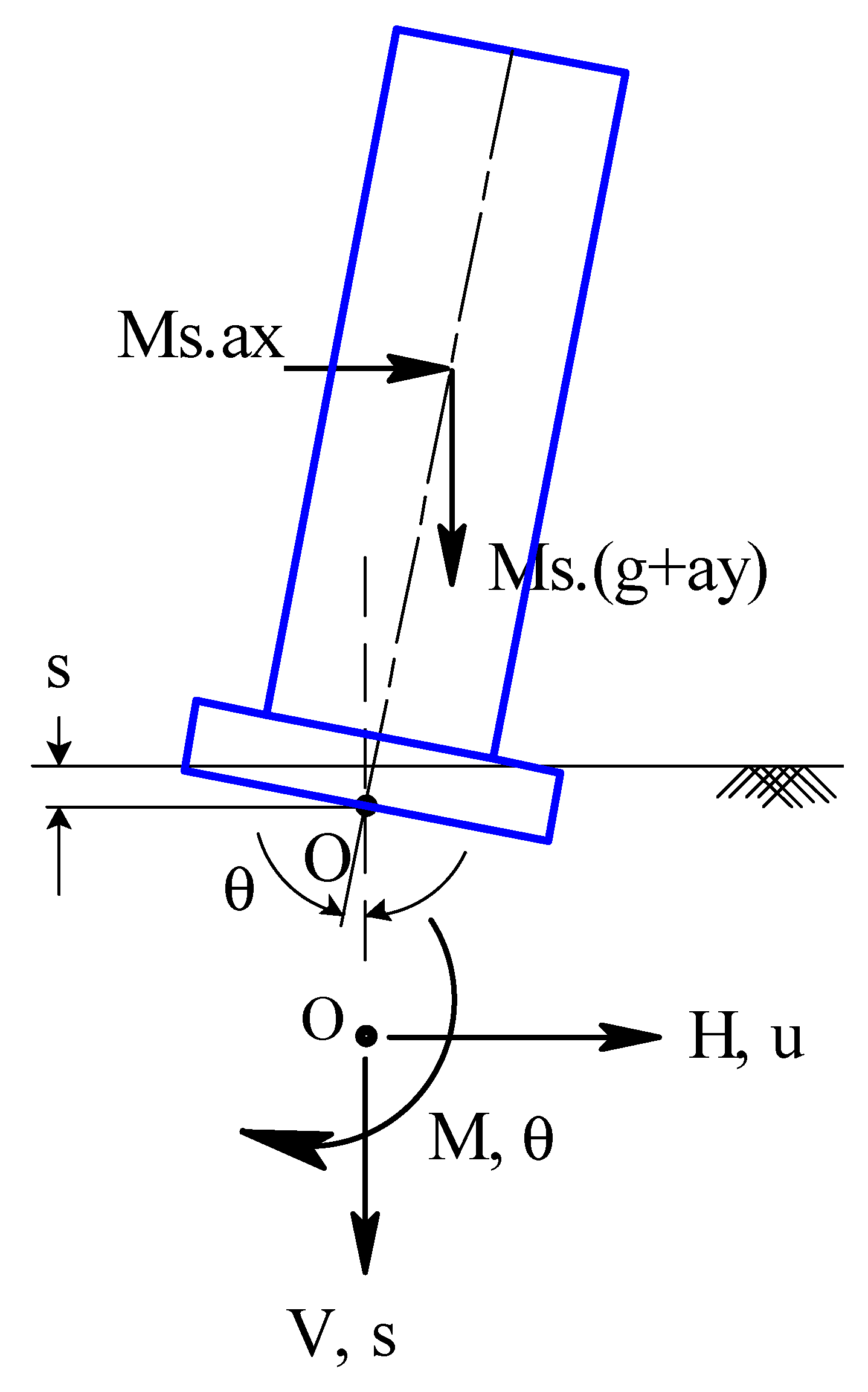
Figure 1 shows the schematic of a rocking structure supported by a shallow foundation and the forces (vertical load (V), horizontal load (H) and moment (M)) and displacements (settlement (s), sliding (u) and rotation (θ)) acting at the soil–footing interface during rocking. The peak rotation of rocking foundation (θpeak) is defined as the absolute maximum rotation experienced by the foundation during earthquake shaking, which is also the same as the peak rotation of the structure, as the footing and structure are rigidly connected. Gajan and Kayser (2019) [15], for example, using parametric studies of numerical simulations, demonstrated that the peak rotation of a rocking foundation is strongly correlated to maximum acceleration of base shaking (amax). The magnitude of rocking-induced rotation of the structure also depends on the slenderness ratio of the rocking system (h/B, where h is the effective height of the structure and B is the width of the footing in the direction of rocking), as h/B predominantly controls the applied moment-to-shear ratio at the footing–soil interface [27]. The other parameters that affect the peak rotation of rocking foundation include critical contact area ratio, rocking coefficient, Arias intensity of earthquake motion, and type of soil [7].
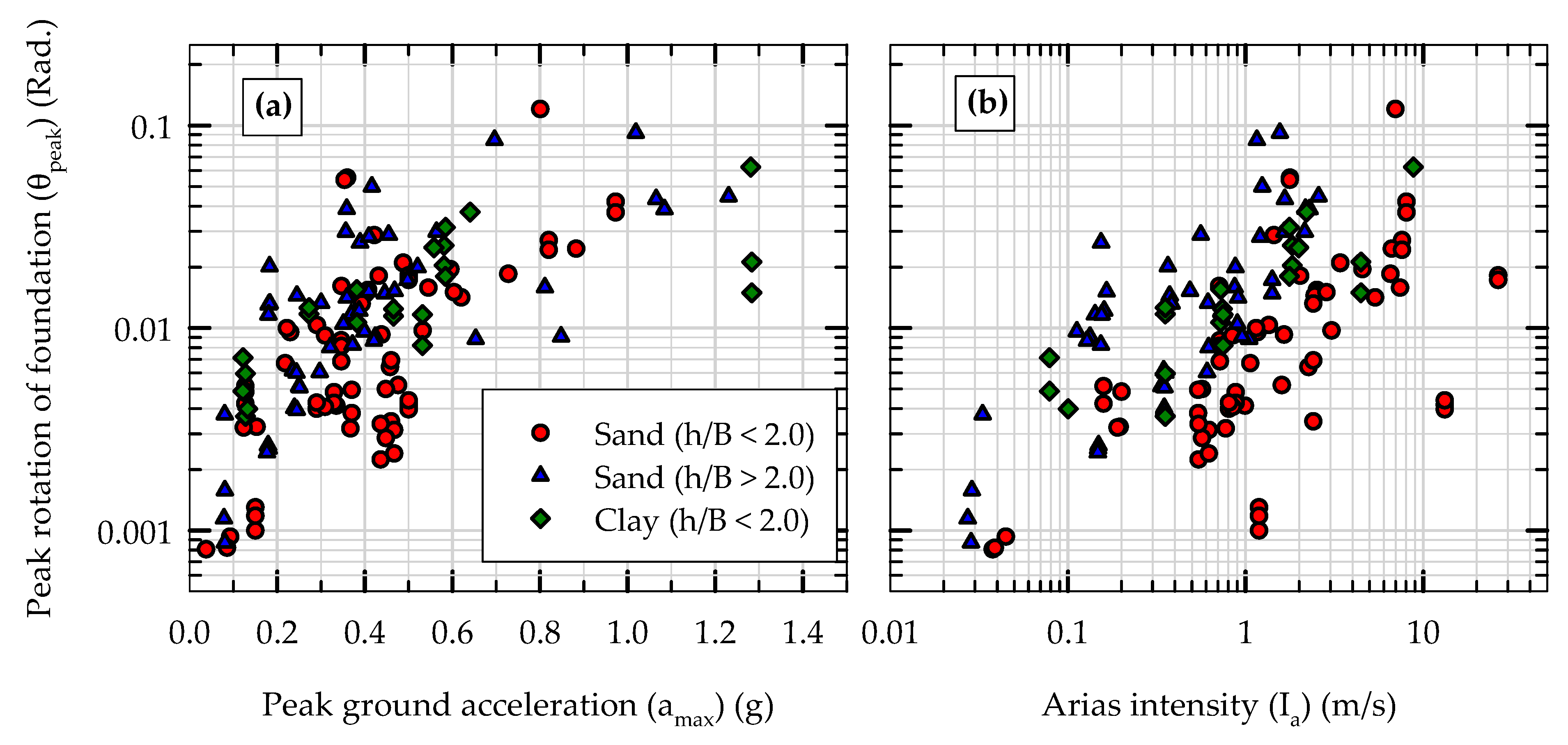
Figure 2a presents the variation of peak rotation of foundation (θpeak) with peak ground acceleration (amax) of earthquake motion for three different clusters of slenderness ratio (h/B) of rocking systems (two sets on sand and one set on clay foundations). It should be noted that for all rocking systems presented in Figure 2 and in this paper, the slenderness ratio (h/B) is greater than 1.0 (i.e., all systems considered are rocking-dominated systems as opposed to sliding-dominated systems). The experimental results presented in Figure 2 were extracted from 140 centrifuge and shaking table experiments on rocking foundations available in a publicly available database (described further in Section 3.1). As can be seen from Figure 2a, in general, and as expected, θpeak increases as amax increases; however, there is scatter in the data. Similarly, though the data are scattered, in general, for a given amax, higher slenderness ratio structure–footing systems rotate more than their lower counterparts, indicating the ability of slender structures to rock more than relatively shorter structures. Figure 2a also shows that rocking systems on clayey soils rotate more than those on sandy soils with the same range of slenderness ratios (1.0 < h/B < 2.0). This behavior is consistent with the clayey soil foundations’ ability to dissipate more seismic energy compared to sandy soils for a given shaking intensity [7].
Figure 2b presents the variation of peak rotation of foundation (θpeak) with Arias intensity (Ia) of earthquake motion for the same data and the same group of rocking foundations (same as in Figure 2a). In addition to the amplitude of shaking acceleration, Ia also includes the effects of frequency content and duration of shaking, and hence it is not a redundant input feature to correlate and predict peak rotation of rocking foundations. The data in both Figure 2a,b, in general, show similar trends, although the scatter in data is slightly higher in Figure 2b. As can be seen from Figure 2b, as Ia increases, the peak rotation of rocking foundation increases, and for a given Ia, peak rotation increases with increasing h/B ratio. It turns out that Ia is the second most important feature after amax in predicting the peak rotation of rocking foundations (presented in Section 5.3: Significance of input features).
Figure 3 shows the schematic of a lumped mass–column–foundation representation of a relatively rigid structure rocking on supporting soil, illustrating the initial (red) and rotated (blue) positions of the structure and footing during rocking. Critical rotation of a rocking structure (θcrit) can be defined as the magnitude of rotation that would possibly cause tipping-over failure of the structure–foundation system during earthquake. Using static equilibrium conditions on the verge of tipping-over failure, the maximum horizontal displacement at the center of gravity of the structure (Δcrit) during earthquake shaking that would cause tipping-over failure can be obtained by,
Δ crit = B B c 2
where Bc is the critical contact width of the footing with the soil (in the direction of shaking) that is required to support applied vertical load (Bc is defined and is correlated to the bearing capacity of a square or rectangular foundation in Section 3.2). The critical rotation (θcrit) can then be defined as,
θ crit = tan 1 Δ crit h
In order to quantify the stability of rocking systems against tipping-over failure during shaking, a factor of safety for tipping over (FSTO) can be defined by comparing the peak rotation with the critical rotation of the rocking system. On the verge of static (limiting) equilibrium during rocking, the factor of safety for tipping-over failure is defined as,
FS TO = θ crit θ peak
Figure 4a presents the variation of factor safety for tipping over (FSTO) with peak ground acceleration (amax) of the earthquake ground motion for different clusters of slenderness ratio (h/B) of the structure–footing systems (the same groups of experiments presented in Figure 2). Figure 4b presents the same dataset with Arias intensity of ground motion (Ia) on the x-axis. It can be seen from Figure 4 that FSTO is as high as 400 during shaking for relatively smaller intensity earthquakes and at least 2.0 or greater for higher intensity earthquakes. As expected, FSTO decreases as amax and Ia increase, and for a given amax or Ia, FSTO decreases as h/B increases. Though there is scatter in the data, none of the FSTO values approach 1.0 (critical FSTO on the verge of tipping-over failure). This is consistent with the experimentally observed behavior that none of the structure–footing systems used in any of these 140 experiments tipped over during shaking. Data also show that the tipping-over stability of rocking foundations is higher on clayey soils compared to sandy soil foundations. This behavior is also consistent with the previous research findings. Sharma and Deng (2019) [28], based on field experiments of rocking foundations on clayey soils, concluded that rocking systems on clay exhibited a re-centering ability that is better than on sand.

3. Experimental Data and Input Features

3.1. Experimental Data

The data and results obtained from five series of centrifuge experiments [2,29,30,31] and four series of shaking table experiments [32,33,34,35] on rocking foundations (altogether 140 individual base-shaking experiments) were utilized in this study. Details of these experiments, including types of soils, types of foundations and structures, types of ground motions, number of shaking events, raw data, and metadata, are available in a database (https://datacenterhub.org/deedsdv/publications/view/529, accessed on 1 August 2022) [5]. The soils used in the experiments can be categorized as competent soils: dry Nevada sand of relative density 40% to 80%, dry Longstone sand of relative density 45% to 90%, and consolidated saturated clay of undrained shear strength 50 kPa to 70 kPa. The foundations used in the experiments were either square or rectangular spread footing shallow foundations and the types of structures used included relatively rigid shear walls and single-degree-of-freedom-type columns supporting a rigid mass at top. It should be noted that nonlinear structures, including flexible beams and columns and multi-degree-of-freedom structures with higher mode effects, were not included in this study. The effects of key rocking system parameters (e.g., critical contact area ratio and rocking coefficient) and earthquake demand parameters (e.g., peak ground acceleration and Arias intensity of ground motion) on the performance of rocking foundations (e.g., peak rotation and permanent settlement), derived from the results obtained from this database, are published in Soundararajan and Gajan (2020) [36] and Gajan et al. (2021) [7].

3.2. Input Features

In order to predict θpeak and FSTO of rocking foundations during shaking using machine learning algorithms, six input features (input parameters) were chosen and are described briefly in the following sections. Further justification for the selection of input features is presented in Section 5.3: Significance of input features.
(i) Critical contact area ratio (A/Ac): A/Ac is, conceptually, a factor of safety for rocking foundation with respect to vertical loading (where A is the total base area of the footing and Ac is the minimum footing contact area with the soil required to support the applied vertical load (V)) [2]. As illustrated in Figure 3, the contact width of the footing with soil (in the direction of shaking) changes during rocking and the critical contact width of the footing (Bc = Ac/L, where L is the dimension of the footing perpendicular to shaking) determines the ultimate bearing capacity (qult) when the contact width reaches Bc. It should be noted that A/Ac = B/Bc for rectangular and square footings with shaking direction parallel to the plan dimension B of the footing. As qult depends on the size and shape of the actual footing–soil critical contact area, an iterative procedure can be used to determine Bc and A/Ac using Equation (4) [2,30].
A A c = q ult   B . L V
(ii) Slenderness ratio of rocking system (h/B): It has been shown that the performance of rocking foundations, in general, depends on the applied moment-to-shear ratio (M/H) at the footing–soil interface due to the coupling between vertical, horizontal and moment loading [27]. The M/H ratio can be approximated to the h/B ratio of the rocking system, where h is the height of center of gravity of the rocking system from the base center point of the footing, as in Equation (5) [27],
h B M H . B
The expectation is that the more slender the rocking system (higher h/B and M/H ratios), the higher the tendency to rock, hence results in relatively greater values for θpeak and possibly smaller values for FSTO.
(iii) Rocking coefficient (Cr): Ignoring the passive resistance of soil in front of a shallow foundation, it has been shown that the ultimate moment capacity of a rocking foundation (Mult) is correlated to A/Ac, V and B, as given by Equation (6) [2].
M ult = V . B 2 · 1 A c A
Cr, is the ratio of the Mult of the foundation to the weight (V) of the structure normalized by the effective height (h) of the structure, as in Equation (7) [30].
C r = B 2 . h · 1 A c A
It should be noted that Cr combines the effects of soil properties and foundation geometry (through A/Ac) with the slenderness ratio (h/B) of the rocking system. For rectangular and square footings, combining Equations (1), (2) and (7) results in the following simplified expression for critical rotation of rocking foundations in terms of rocking coefficient,
θ crit = tan 1 C r
Using meta-analysis of experimental data from multiple studies, Gajan et al. (2021) [7] have shown that many performance parameters of rocking foundations, including peak rotation and factor of safety for tipping-over, depend mainly on A/Ac, h/B, and Cr of the rocking system.
(iv) Peak ground acceleration (amax): amax is the absolute maximum horizontal acceleration of the earthquake ground motion. As the peak rotation (θpeak) of a rocking system is instantaneous (due to the reversing nature of the seismic shaking and the self-centering characteristic of rocking shallow foundations) and most likely caused by the maximum acceleration spike, amax was chosen as the key input feature representing the seismic demand. In addition, amax is one of the dominant indicators of the severity of the earthquake motion and θpeak is expected to increase, up to a certain limit, as amax increases.
(v) Arias intensity of ground motion (Ia): Ia is calculated using numerical integration in the time domain via Equation (9) [37],
I a = π 2 . g 0 t fin a t 2 dt
where g is the gravitational acceleration, a(t) is the horizontal ground shaking acceleration time history, and tfin is the duration of earthquake ground motion. Ia includes the combined effects of amplitude, duration, frequency content, and number of cycles of earthquake loading. As the rotational stiffness of rocking foundation typically degrades with number of cycles and duration of loading [1,2], θpeak and FSTO of rocking foundation are expected to depend on Ia.
(vi) Type of soil: A binary parameter called “Type” was used to separate sandy soil foundations from clayey soil foundations (i.e., Type takes the value of either 0 or 1). Experimental results presented in Figure 2 and Figure 4 show that θpeak and FSTO depend on the type of soil, to some extent.
All the input feature parameters were calculated for 140 individual experiments from the above-mentioned database and presented in Soundararajan and Gajan (2020) [36] and Gajan et al. (2021) [7], and hence not repeated in this paper. Figure 5 presents the probability distributions (in terms of frequency of occurrence in experiments) of four major input features (A/Ac, Cr, amax, and Ia) along with their mean and coefficient of variation (COV). The input features presented in Figure 5 were lumped into five groups (intervals) in order to plot the frequency plots (however, their individual values were used in the development of machine learning models). As can be seen from Figure 5, the experimental data and results utilized in the development of the machine learning models in this study cover a wide range of rocking system capacity parameters and earthquake ground motion demand parameters. It should be noted that the variation (numerical range) in θpeak, FSTO, and Ia is relatively high (Figure 2, Figure 4 and Figure 5). For this reason, these three parameters were transformed to logarithmic values (base 10) before the training and testing phases of the machine learning models. In addition, in order to make reliable predictions using models developed by different machine learning algorithms, all the input feature data were normalized so that each input feature value varied between 0.0 and 1.0.

4. Machine Learning Algorithms

4.1. K-Nearest Neighbors Regression (KNN)

The inductive bias of the KNN algorithm is based on the assumption that when input data points are plotted as vectors in multi-dimensional input feature space, the data points that lie closer together share similar properties (i.e., similar output or prediction values). If there are hidden relationships between multiple input features and the prediction variable, the KNN model is able to learn those relationships through the training data. In this study, the Euclidean distance measure in n-dimensional space was used to calculate the distance between two data instances (n = 6 in this study; one for each input feature). In KNN, the entire training data are stored in the model during the training phase. When a test data instance is fed as input, the KNN algorithm runs through the entire training dataset and finds k number of training instances that are closer to the test instance. The distance-weighted KNN regression model weighs the output values by the inverse of their distance from the test data point to its nearest neighbors and produces an output that is the weighted average of the output values of the nearest neighbors (i.e., closer neighbors of a test data point will have a greater influence on the output than neighbors that are further away). The optimum value of k of KNN model was found to be in between 3 and 5 for the problem considered and k = 3 was used for all cases presented in this paper, except in the hyperparameter tuning phase of the models (presented later).

4.2. Support Vector Regression (SVR)

The objective of original support vector machine (SVM) algorithm for classification is to find a hyperplane in an n-dimensional input space that distinctly separates the data points. The margin (ϵ) is the distance from the hyperplane to the closest data point (support vector) in n-dimensional space. The major difference between SVM and SVR is that whereas the SVM classification algorithm tries to fit the largest possible margin between different classes while limiting margin violations of data points, the SVR algorithm tries to fit as many training data instances as possible within the margin while limiting margin violations of data points. The inductive bias of the SVR algorithm is that it assumes that the data points that have distinct characteristics tend to be separated by wide margins. The major parameter of SVR algorithm is the kernel function that is used to map (transform) the data instances (input data) into n-dimensional space. The radial basis function (RBF) kernel was used in this study as it is the most widely used kernel in SVR and it has the flexibility of dealing with nonlinear data [16]. Since complex, nonlinear data cannot be accommodated perfectly by a hyperplane and a margin, wiggle room was allowed for the margin. A hyperparameter called the cost parameter or penalty parameter (C) defines the magnitude of this wiggle room across all dimensions in input space. The optimum value of C of the SVR model was found to be 20 for the problem considered and C = 20 (with ϵ = 0.1) was used for all cases presented in this paper, except in the hyperparameter tuning phase (discussed further in the hyperparameter tuning section).

4.3. Random Forest Regression (RFR)

The decision tree regression (DTR) algorithm uses a supervised learning technique to build a tree-like data structure by employing a top-down, greedy search through the space of possible branches using information gain as a measure of reduction in uncertainty in training data. The inductive bias of the DTR algorithm is that the trees that place high information gain attributes close to the root are preferred over those that do not (shorter trees are preferred over longer trees). A random forest regression (RFR) model is an ensemble model that fits multiple base DTR models, each on random subsets of the original training dataset and using random input features, and then aggregates their individual predictions on the testing dataset by averaging to form a final prediction. The major hyperparameter of the DTR model is the maximum depth of the tree, and the optimum value for the maximum depth of the tree was found to be 6 for the data analyzed (presented later). In the RFR model, each individual base DTR model may have a higher bias than if it were trained on the original training dataset, but introduction of randomness and aggregation reduces both bias and variance. In other words, the introduction of randomness in input training data (random subset of training data, random input features, and random size individual trees) reduces the uncertainty in final predictions on test data. For optimum performance of the RFR model, the maximum number of random input features to consider when considering a split is limited to 2 (a hyperparameter) (randomly chosen 2 features out of total 6 features) and the optimum value for the number of trees in the ensemble was found to be 100 (described further in the hyperparameter tuning section).

5. Results and Discussion

The initial evaluation of machine learning models using a randomly selected pair of training and testing datasets is presented first and it is followed by the results of hyperparameter tuning of the models, input feature importance analysis using multiple random training datasets, and repeated k-fold cross validation tests of the models using multiple random splits of training and testing datasets. The metrics used to evaluate the performance of machine learning models developed in this study include mean absolute error (MAE) and mean absolute percentage error (MAPE), and they are defined as,
MAE = 1 n i = 1 n y i y i
MAPE = 1 n i = 1 n y i y i y i
where y is the actual output value (experimental data), ỹ is the predicted output value, and the subscript “i” runs from 1 up to the number of predictions (n). As the experimental data considered covers a significant range of values with scatter (Figure 2 and Figure 4), MAE and MAPE are preferred and chosen over the commonly used root mean square error measure in machine learning models. In addition, while MAE measures the error in terms of the absolute values of output parameter, MAPE is independent of the absolute values and units of the output parameter (by normalization). For the purpose of comparisons, a multivariate linear regression (MLR) model was also developed using the same input features and supervised learning technique. Since the MLR model is a linear, parametric model, it was used as the baseline model for comparison of performances of different machine learning models. All the machine learning models in this study were developed using the implementations of the algorithms available in “scikit-learn” library of modules in Python (https://scikit-learn.org/stable/, accessed on 1 August 2022).

5.1. Initial Evaluation of Models

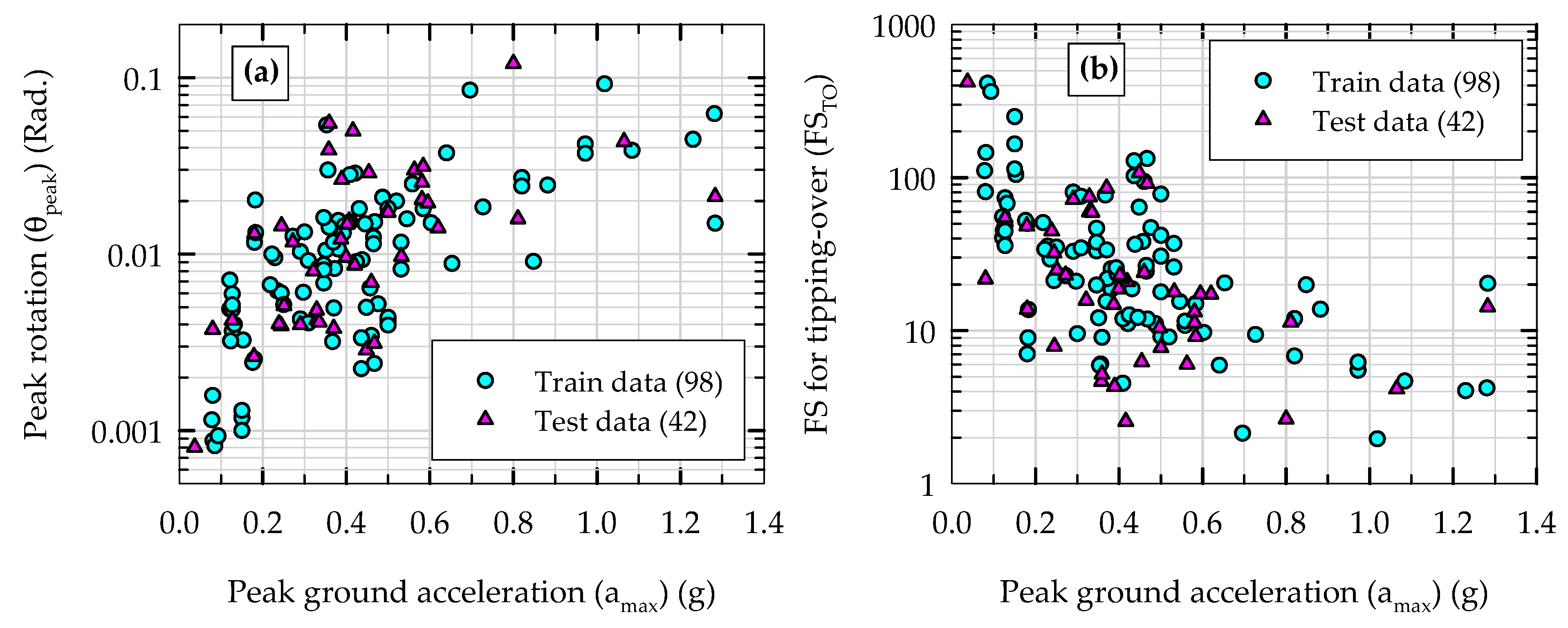
Altogether 140 experimental data (instances) were extracted from the above-mentioned database and are split into two groups for the purpose of initial training (supervised learning) and testing of machine learning models. A 70–30% split was used to randomly create the training dataset (98 instances) and testing dataset (42 instances) using the train-test-split function available in “scikit-learn” library of modules in Python. The 70–30% split is similar to the rule of thumb methods commonly used in supervised machine learning. Note that the random-state variable in this function was kept constant for this splitting of data for initial training and testing of all the models (i) to ensure consistency between different machine learning models and (ii) to ensure repeatability of results. Figure 6a presents this split of data in θpeak versus amax space, while Figure 6b presents the same split of data in FSTO versus amax space. This train–test split was created randomly, and as a result, both training and testing sets of data cover a wide range of values for all the parameters considered reasonably well. The machine learning models were first trained independently using the training dataset and then tested using the testing dataset. It should be noted that as the total number of data instances (140) is relatively small, a separate validation set was not used in this study; instead, hyperparameter tuning was carried out using multiple runs of the training dataset (presented in Section 5.2).
The variations in predicted peak rotation (θpeak) with the corresponding experimental θpeak values on top of 1:1 prediction-to-experiment comparison lines during the testing phase are presented in Figure 7 for four ML models: (a) KNN, (b) SVR, (c) DTR, and (d) RFR. Also included in Figure 7 are the testing MAPE values of the predictions of each model. Note that the values of hyperparameters for all the models are kept at their optimum values (obtained from the hyperparameter tuning phase, described in the next section): k = 3 in KNN model, C = 20 and ε = 0.1 in SVR model, maximum depth of tree = 6 in DTR model, and number of trees = 100 and maximum number of random input features used in each tree = 2 in RFR model. As can be seen from Figure 7, the KNN model outperforms the other three models in terms of the MAPE of prediction (0.33) during the initial testing phase, and it is followed by the SVR model (MAPE = 0.4). The DTR model (a single decision tree) results in a MAPE of 0.48 during testing phase; however, when 100 decision trees are combined as a random forest in the RFR model, the accuracy of the model improves slightly (MAPE = 0.44). To investigate the variance in individual predictions of the models, the standard deviations of the absolute percentage error (APE) in model predictions were also calculated. The standard deviations of the APE in predictions of θpeak of KNN, SVR, DTR, and RFR models are 0.23, 0.38, 0.42, and 0.31, respectively. This indicates that in terms of variance in predictions of θpeak, KNN is still the best out of the four models, and that the RFR model is better than both SVR and DTR in terms of variance in predictions.
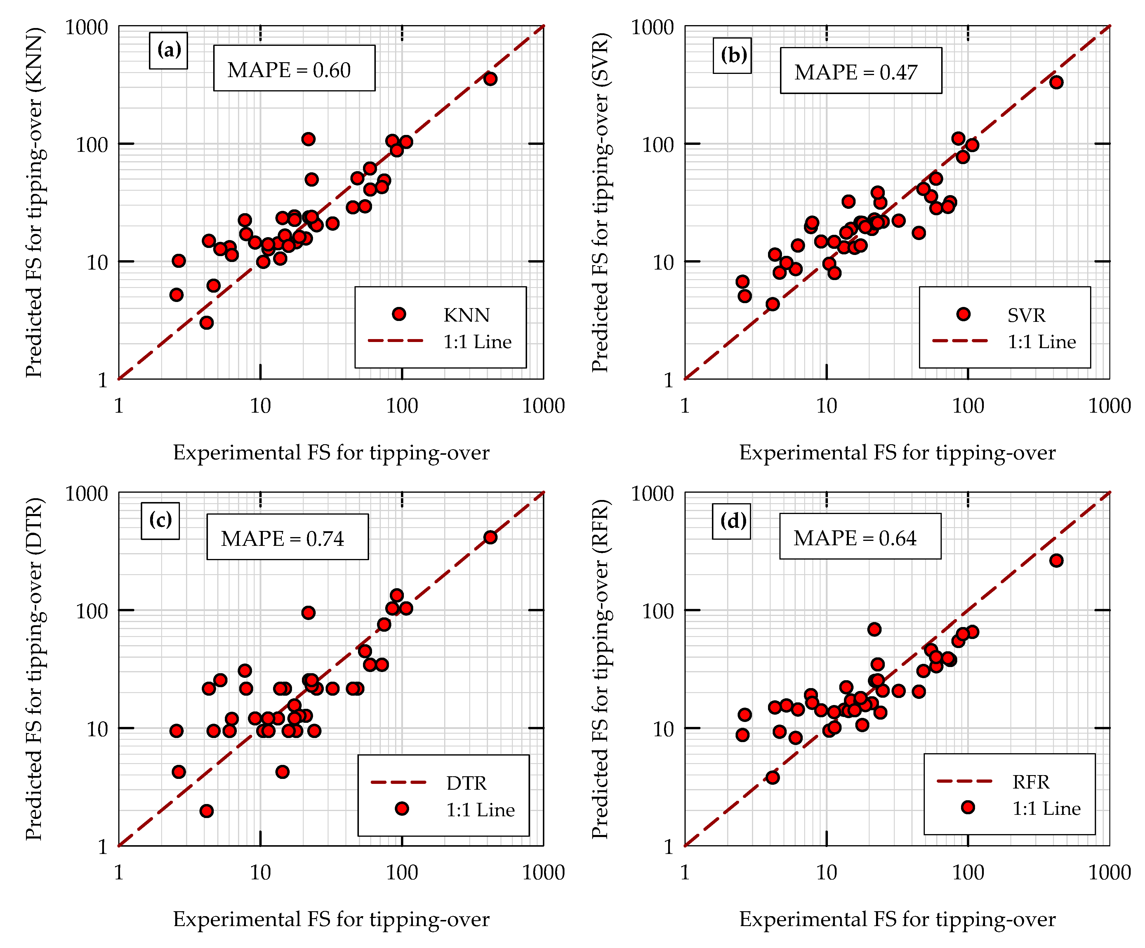
Figure 8 presents the comparisons of different model predictions during the testing phase with experimental results for factor of safety for tipping over (FSTO) in the same format as in Figure 7. The hyperparameters used for all four ML models are the same as above (the same as the ones used for the prediction of θpeak). For the prediction of FSTO, the SVR model turned out to be the best model during this initial testing phase (MAPE = 0.47). The KNN model (MAPE = 0.6) seems to have more deviations in predictions and is unable to compete with the SVR model. However, as can be seen from Figure 8, the performance of the KNN model is still better than the DTR model in terms of accuracy of predictions. As in the case with θpeak, by combining 100 decision trees together as an ensemble model, the RFR model was able to improve the accuracy (MAPE = 0.64) while reducing the variance in predictions of FSTO compared to the DTR model. The standard deviations of the absolute percentage errors (APE) in predictions of the FSTO of the KNN, SVR, DTR, and RFR models are 0.84, 0.48, 1.04, and 0.82, respectively. This indicates that in terms of variance in predictions of FSTO, SVR is still the best out of the four models, and that the performance of the KNN and RFR models are relatively similar or comparable to each other and better than the DTR model in terms of variance in predictions. Note that, for all four machine learning models, the MAPE values and variance in the predictions of FSTO (Figure 8) are consistently higher than those of θpeak (Figure 7).
It should be noted that after the initial training phase of the ML models, in order to check the applicability of the models to represent the training data and to quantify what the models learned from the training data, all the machine learning models were first tested using the same training dataset (i.e., how well the models predict the same data that are used to train the models; referred to as training error). Another reason for this exercise was to make sure that the models did not overfit the training data, by comparing the testing error with the training error. Figure 9 presents an all-error comparison for different scenarios to compare and contrast the performance of different machine learning models based on the MAPE in the prediction of θpeak and FSTO in initial training and testing phases of the models. Also included in Figure 9 are the MAPE values of a multivariate linear regression (MLR) machine learning model developed as a baseline model using the same input features and the same training and testing datasets. MLR is a linear, parametric model, where a hyperplane is used to model the relationship between the output and multiple input variables. Based on the MAPE values of the models on training and testing data, it is apparent that all four nonlinear nonparametric machine learning models developed in this study (KNN, SVR, DTR, and RFR) perform better than the baseline MLR model. Among the four nonparametric models, KNN, SVR and RFR models perform better than DTR model in terms of accuracy of predictions (lower testing MAPE values). For all models, the testing MAPE values are greater than those in the training phase. This trend is a typical characteristic of machine learning models, especially when the size of the data is relatively small. This also confirms that the ML models developed in this study do not overfit the training data. The repeated k-fold cross validation test results (based on complete random shuffling and splitting of data) are presented later (Section 5.4) to complement this error comparison.

5.2. Hyperparameter Tuning of Models

For each ML model, the key hyperparameters were tuned by minimizing the MAPE values obtained during the initial testing phase of models (testing error). Hyperparameter tuning was carried out (i) to investigate the sensitivity of model predictions to their hyperparameters, (ii) to determine the optimum values of these parameters for the problem considered and data analyzed, and (iii) to ensure that the models neither overfit nor underfit the training data. It should be noted that the hyperparameter tuning was carried out separately for the predictions of θpeak and FS
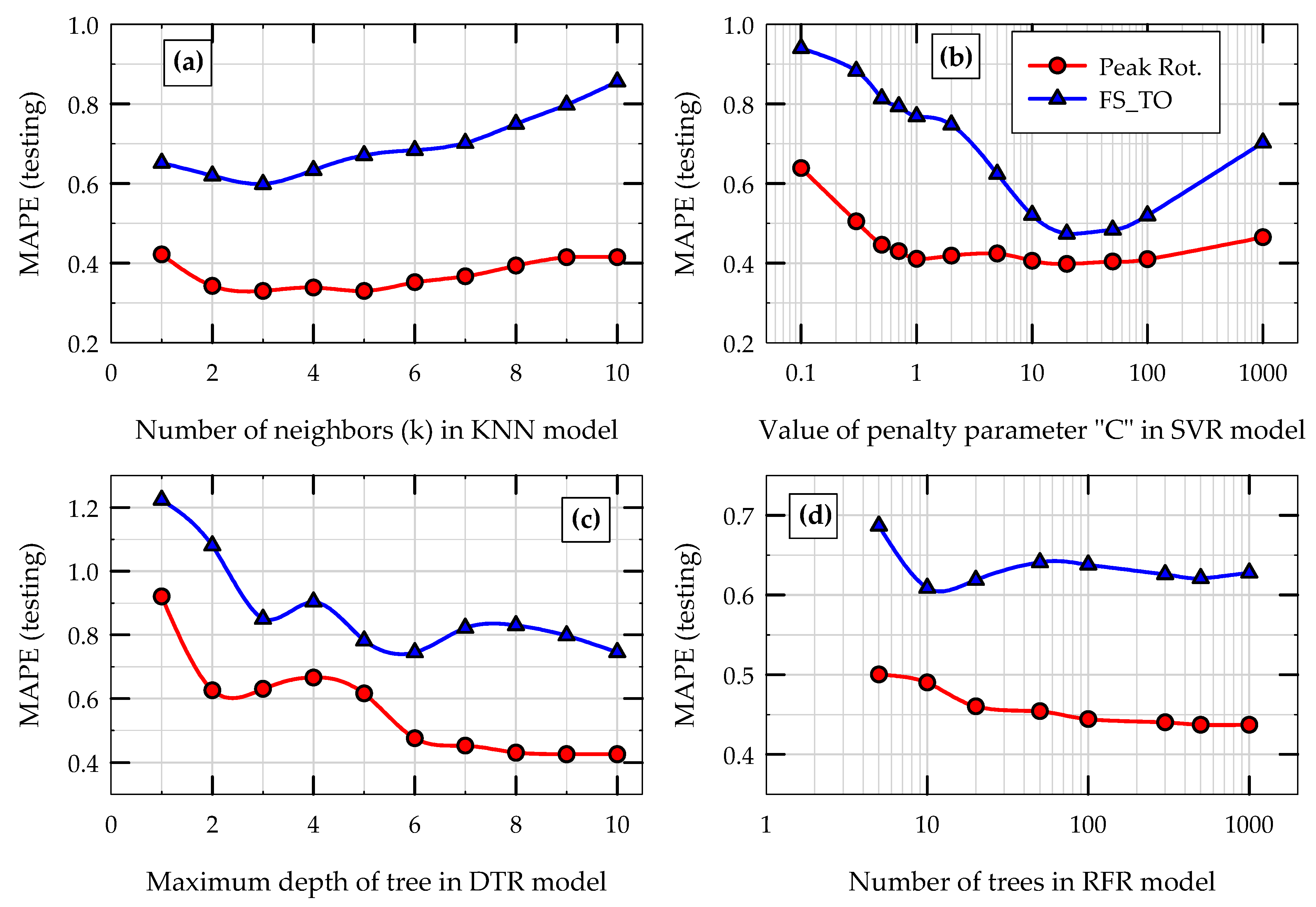
TO. The number of nearest neighbors (k), the cost or penalty parameter (C), the maximum depth of the tree, and the number of trees in random forest were varied for the KNN, SVR, DTR, and RFR models, respectively, and the corresponding MAPE values of predictions were calculated. The variations of testing MAPE values in the predictions of θpeak and FSTO with the corresponding hyperparameters are presented in Figure 10 for all four nonlinear ML models.
For both θpeak and FSTO, the testing MAPE of the KNN model first decreases as the number of nearest neighbors considered (k) increases and then increases as k increases further (Figure 10a). This is a typical behavior of the KNN algorithm when tested with previously unseen test data. The minimum MAPE during testing was obtained when k was equal to 3 for θpeak and when k was in between 3 and 5 for FSTO. Based on this observation and to be consistent, k = 3 was taken as the optimum value for KNN algorithm for both θpeak and FSTO. Any value smaller than the optimum for k would overfit the training data and any value greater than the optimum for k would underfit the training data. Similar to the KNN model, the MAPE during the testing phase of SVR model first decreases and then increases as C increases (Figure 10b). It should be noted that the value of the margin (ϵ) in SVR model was kept at 0.1 for all cases. Neither a very small value for C (underfitting the training data) nor a very high value for C (overfitting the training data) is preferred. For both θpeak and FSTO, the optimum value of C was found to be 20.
Similar to the concept in the KNN and SVR models, for the DTR model (Figure 10c), neither a very shallow tree (underfitting the training data) nor a very deep tree (overfitting the training data) is preferred and an optimum value for maximum depth of the tree is needed. Based on the trend shown in Figure 10c, the optimum value for the maximum depth of tree of DTR model was chosen to be 6 for both θpeak and FSTO. For the RFR model, as can be seen from Figure 10d, the testing MAPE decreases as the number of trees in the random forest increases, indicating that the accuracy of the model increases with the number of trees (this is more apparent for the prediction of θpeak). It should be noted that the maximum number of random features to be considered was kept at 2 and the maximum depth of individual trees was kept at 6 for all trees in the random forest. After about 100 trees in the forest, the MAPE of the RFR model does not seem to decrease further, indicating that the optimum number of trees required is around 100.

5.3. Significance of Input Features

The implementation of the RFR model in the “scikit-learn” library of modules in Python has a function called “feature-importances” that outputs the relative importance of each input feature. This function measures a feature’s importance by looking at how much the tree nodes that use that feature reduce uncertainty in data on average (across all trees in the forest) [16,17]. The function computes this score for each feature after training, then it normalizes the results so that the sum of all feature importance values is equal to 1.0.
To investigate the significance of input features, twenty different RFR models were developed for both θpeak and FSTO by randomly selecting different sets of training data each time (by changing the random state variable), and the feature importance values were obtained for each random forest. The average values of the feature importance (as boxes) along with their standard deviations (as error bars) are presented in Figure 11a,b for the prediction of θpeak and FSTO respectively. As can be seen from Figure 11, the effects of different input features on both performance parameters (peak rotation and factor of safety for tipping over) are remarkably similar and consistent, verifying the inter-relationship between the two performance parameters. As expected and consistent with the previously published experimental results [7], earthquake ground motion intensity parameters (amax and Ia) have the most influence (30% to 35%) on both performance parameters. Three rocking foundation capacity parameters considered in this study as input features (A/Ac, h/B, and Cr) have quantitatively similar influence (about 10% each) on both performance parameters. The type of soil alone (sand or clay) does not have considerable influence on the performance parameters (less than or around 5% feature importance). These results and observations suggest that the earthquake ground motion intensity parameters contribute more to model predictions than the rocking system capacity parameters and type of soil (in other words, the peak rotation and tipping-over stability of rocking foundations are more sensitive to earthquake demand parameters than the properties of soil, foundation, and structure). The type of soil may be considered as a redundant input feature for the problem considered here; however, it should be noted that the shear strength of soil is already included in A/Ac and Cr through bearing capacity of soil.

5.4. Repeated K-Fold cross Validation Tests of Models

The k-fold cross validation test is a technique for evaluating the performance of machine learning models on multiple, different train–test splits of dataset. It provides a measure of how good the model performance is both in terms of accuracy and variance. In k-fold cross validation, the entire dataset is randomly split into k number of subsets called folds, and the ML model is first trained using (k − 1) folds of data and is tested using the remaining fold. This process is repeated k times, picking a different testing fold every time. A single run of k-fold cross validation (a single value for k) may result in noisy results for model error (MAE and MAPE) and hence multiple runs are carried out by varying k (number of folds) and by using random sampling each time. In this study, the complete dataset was randomly shuffled and split into different groups of train–test sets for k = 5 and 7. On top of this, for each of the 5-fold and 7-fold cross validations, the process was repeated three times (number of repeats = 3) with different randomization of the data in each repetition (repeated k-fold cross validation). With this setup, for each model, the repeated 5-fold and repeated 7-fold cross validation tests yielded 15 and 21 values, respectively, for k-fold testing of MAE and MAPE.
Figure 12 presents the results of MAPE of predictions of peak rotation in (a) repeated 5-fold cross validation tests and (b) repeated 7-fold cross validation tests for three nonlinear ML models (KNN, SVR, and RFR) along with the linear, baseline MLR model. In each case, the results obtained for testing MAPE are plotted in the form of boxplots. For each ML model, the boxplot plots the average of MAPE (triangles), median of MAPE (the horizontal line inside the box), 25th and 75th percentile values of MAPE (bottom and top edges of the box), and the 10th and 90th percentile values of MAPE (bottom and top horizontal lines outside the box). As can be seen from Figure 12a,b, for all four ML models, the average values of MAPE in repeated 5-fold and 7-fold cross validation tests are remarkably close to each other (0.75 and 0.76 for MLR, 0.48 and 0.48 for KNN, 0.46 and 0.46 for SVR, and 0.53 and 0.51 for RFR), highlighting the overall consistency of all ML models developed in this study. The average MAPE values of all three nonlinear ML models (0.46 to 0.53) are smaller than that of the baseline MLR model (0.75). The average total variance in MAPE (the average of the difference between two extreme values of MAPE in 5-fold and 7-fold cross validation) of the KNN, SVR, and RFR models are 0.2, 0.3 and 0.32, respectively (the corresponding variance value of MLR is 0.46). In general, lower average MAPE (more accurate) and lower variance in MAPE (less sensitive to differences in training dataset) are preferred. Based on these results and observations, it can be concluded that for the prediction of peak rotation of rocking foundations, the three nonlinear models developed in this study perform much better than the linear MLR model, and that among the nonlinear models, the performance of the KNN model is slightly better than the other two.
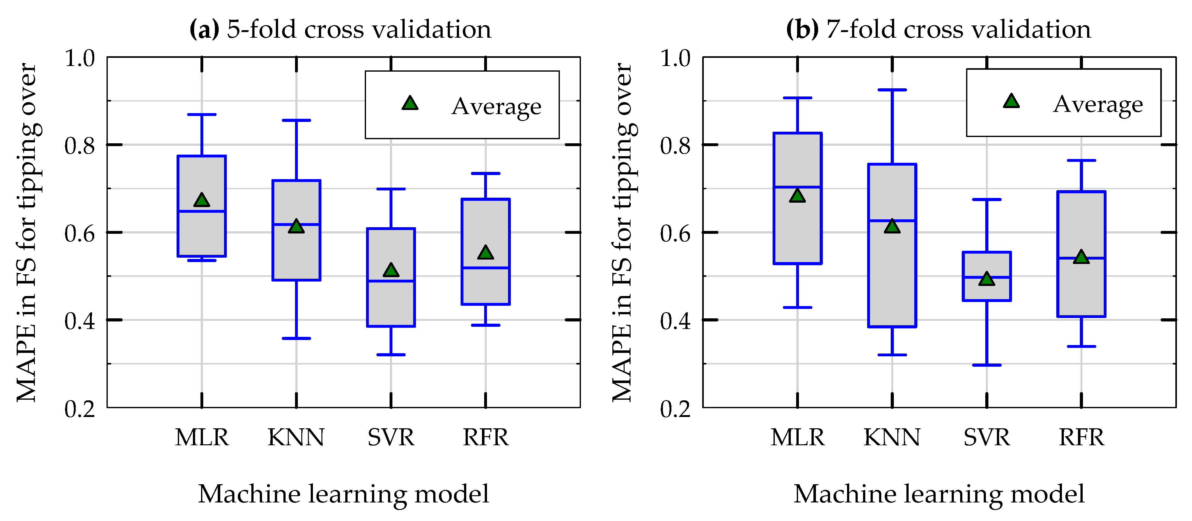
Figure 13 presents the results of MAPE of predictions of factor of safety for tipping over in (a) repeated 5-fold cross validation test and (b) repeated 7-fold cross validation tests for three nonlinear ML models along with the baseline MLR model. The observed trends in Figure 13 (for FSTO) are similar to those of in Figure 12 (for θpeak), except that the average and variance of MAPE in model predictions are slightly higher for FSTO. Similar to the prediction of θpeak, for all four ML models, the average values of MAPE in repeated 5-fold and 7-fold cross validation tests are remarkably close to each other for the prediction of FSTO as well (0.67 and 0.68 for MLR, 0.61 and 0.61 for KNN, 0.51 and 0.49 for SVR, and 0.55 and 0.54 for RFR). As in the case with peak rotation, the average MAPE values of all three nonlinear ML models for the prediction of FSTO (0.49 to 0.61) are smaller than that of baseline MLR model (0.67). The average total variance in MAPE of KNN, SVR, and RFR models are 0.55, 0.37, and 0.38, respectively. Based on these observations, it can be concluded that for the prediction of FSTO of rocking foundations, the three nonlinear models developed in this study perform better than the linear MLR model, and that among the nonlinear models, the performance of the SVR model is better than the other two.
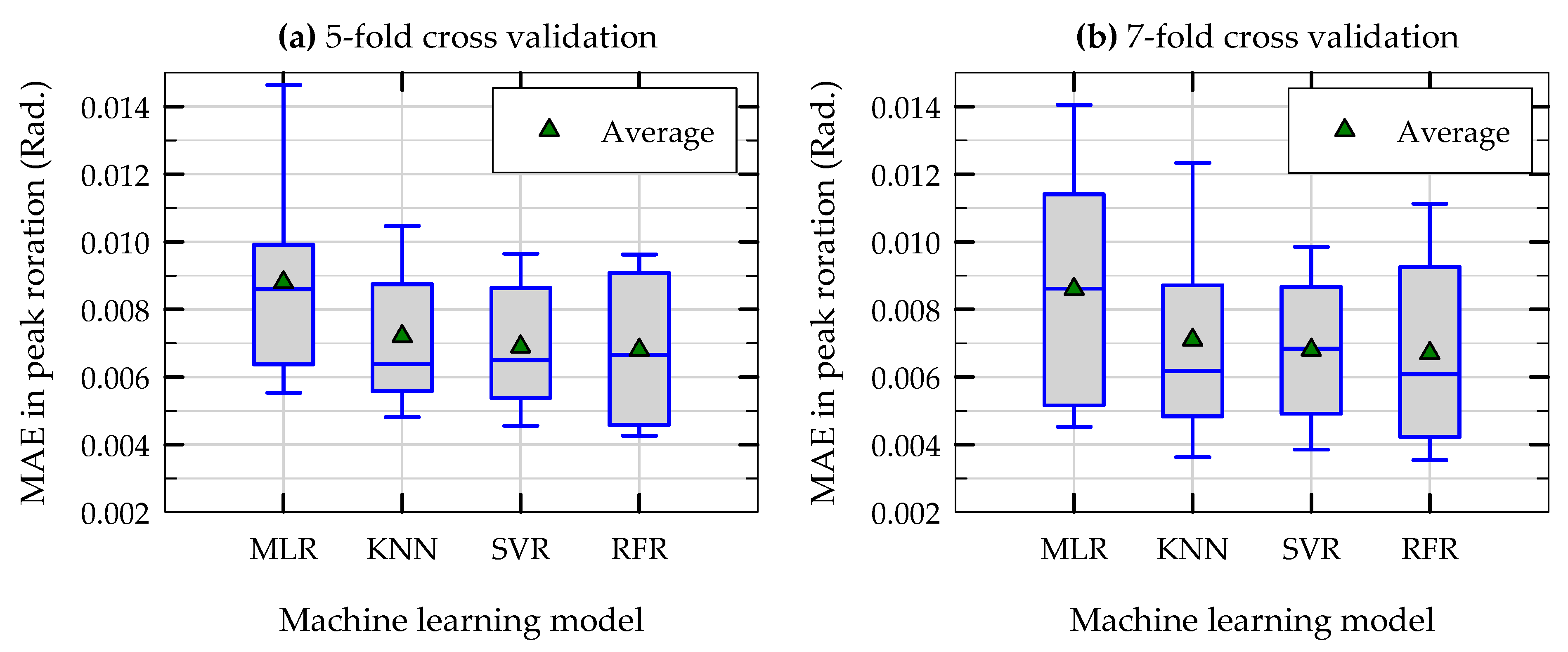
Figure 14 presents the results of MAE of predictions of peak rotation in (a) repeated 5-fold cross validation tests and (b) repeated 7-fold cross validation tests for three nonlinear ML models along with the baseline MLR model. A similar trend is observed for MAE of predictions of different models (similar to the trend observed for MAPE of predictions of peak rotation presented in Figure 12): the performance of all three nonlinear ML models in terms of the average and variance of MAE of their predictions of θpeak are better than that of the linear MLR model. The average MAE values of the three nonlinear ML models for peak rotation is around 0.007, indicating that the rocking-induced peak rotation can be predicted with an average accuracy of 0.007 radians (0.4 degrees). This error limit corresponds to a lateral displacement (at effective height of structure) that is approximately equal to 0.7% of the effective height of the structure.

6. Summary and Conclusions

Three nonlinear machine learning algorithms (KNN, SVR, and RFR) were used to develop data-driven, predictive models for peak rotation (θpeak) and factor of safety for tipping-over failure (FSTO) of rocking foundations during seismic loading using a supervised learning technique. The input features to the machine learning algorithms included critical contact area ratio of foundation (A/Ac); slenderness ratio (h/B) and rocking coefficient (Cr) of rocking system; peak ground acceleration (amax) and Arias intensity (Ia) of earthquake ground motion; and a categorical binary feature that separates sandy soil foundations from clayey soil foundations. The models were trained and tested using centrifuge and shaking table experimental results on rocking foundations and the performances of the models were compared with one another and with a baseline MLR model in terms of accuracy and variance of their predictions using MAPE and MAE. In addition to initial evaluation of the models using a 70–30% train–test split of data instances, hyperparameter tuning of models, input feature importance analysis, and repeated 5-fold and 7-fold cross validation tests of the models using random sampling were also carried out. Based on the results presented in this paper, the following major conclusions are derived.
  • Based on the results obtained from repeated k-fold cross validation tests of ML models, the three nonlinear ML models developed in this study (KNN, SVR, and RFR) outperform the baseline linear MLR model in terms of accuracy and variance in predictions of θpeak and FSTO of rocking foundations.
  • The overall average MAPE values of the three nonlinear models in the predictions of θpeak are in between 0.46 and 0.53, while the corresponding MAPE value of the baseline MLR model is around 0.75. Similarly, the overall average MAPE values of the three nonlinear models in the predictions of FSTO are in between 0.5 and 0.6, while the corresponding MAPE value of the baseline MLR model is around 0.68.
  • Based on the overall average and variance of MAPE of predictions in repeated k-fold cross validation tests, it can be concluded that for the prediction of θpeak, the KNN model performs slightly better than the other two nonlinear ML models, whereas for the prediction of FSTO, the SVR model performance is better than the other two nonlinear ML models.
  • The overall average MAE values in predictions of all three nonlinear ML models are around 0.007, indicating that the peak rotation of rocking foundations during seismic loading can be predicted with an average accuracy of 0.4 degrees. This error limit corresponds to a lateral displacement (at effective height of structure) that is approximately equal to 0.7% of the effective height of the structure.
  • Based on the feature importance values obtained from multiple RFR models, it can be concluded that the chosen input features capture θpeak and FSTO of rocking foundations satisfactorily, and that these performance parameters are more sensitive to ground motion demand parameters than to rocking system capacity parameters or type of soil.
  • Hyperparameter tuning of the ML models was used to obtain the optimum values of the hyperparameters, and the results show that the ML models developed in this study neither underfit nor overfit the training data.
  • The data-driven predictive models developed in this study can be used in combination with other mechanics-based models to complement each other in modeling of rocking foundations in practical applications. One such approach would be theory-guided data science, an emerging field that combines physics/mechanics with machine learning [38].

Funding

This research received external funding from the US National Science Foundation (award number CMMI-2138631).

Institutional Review Board Statement

Not applicable.

Informed Consent Statement

Not applicable.

Data Availability Statement

The data presented in this study are available on request from the corresponding author.

Acknowledgments

The author acknowledges the National Science Foundation (NSF) for funding the research presented in this paper through award number CMMI-2138631.

Conflicts of Interest

The author declares no conflict of interest.

References

  1. Gajan, S.; Phalen, J.D.; Kutter, B.L.; Hutchinson, T.C.; Martin, G. Centrifuge modeling of load-deformation behavior of rocking shallow foundations. Soil Dyn. Earthq. Eng. 2005, 25, 773–783. [Google Scholar] [CrossRef]
  2. Gajan, S.; Kutter, B.L. Capacity, settlement, and energy dissipation of shallow footings subjected to rocking. J. Geotech. Geoenviron. 2008, 134, 1129–1141. [Google Scholar] [CrossRef]
  3. Paolucci, R.; Shirato, M.; Yilmaz, M.T. Seismic behavior of shallow foundations: Shaking table experiments versus numerical modeling. Earthq. Eng. Struct. Dyn. 2008, 37, 577–595. [Google Scholar] [CrossRef]
  4. Anastasopoulos, I.; Gazetas, G.; Loli, M.; Apostolou, M.; Gerolymos, N. Soil failure can be used for seismic protection of structures. Bull. Earthq. Eng. 2010, 8, 309–326. [Google Scholar] [CrossRef]
  5. Gavras, A.G.; Kutter, B.L.; Hakhamaneshi, M.; Gajan, S.; Tsatsis, A.; Sharma, K.; Kouno, T.; Deng, L.; Anastasopoulos, I.; Gazetas, G. Database of rocking shallow foundation performance: Dynamic shaking. Earthq. Spectra 2020, 36, 960. [Google Scholar] [CrossRef]
  6. Hakhamaneshi, M.; Kutter, B.L.; Gavras, A.G.; Gajan, S.; Tsatsis, A.; Liu, W.; Sharma, K.; Pianese, G.; Kouno, T.; Deng, L.; et al. Database of rocking shallow foundation performance: Slow-cyclic and monotonic loading. Earthq. Spectra 2020, 36, 1585–1606. [Google Scholar] [CrossRef]
  7. Gajan, S.; Soundararajan, S.; Yang, M.; Akchurin, D. Effects of rocking coefficient and critical contact area ratio on the performance of rocking foundations from centrifuge and shake table experimental results. Soil Dyn. Earthq. Eng. 2021, 141, 106502. [Google Scholar] [CrossRef]
  8. ASCE/SEI Standard 41-13; Seismic Evaluation and Retrofit of Existing Buildings. American Society of Civil Engineers (ASCE): Reston, VA, USA, 2014. [CrossRef]
  9. Kelly, T.E. Tentative seismic design guidelines for rocking structures. Bull. N. Z. Soc. Earthq. Eng. 2009, 42, 239–274. [Google Scholar] [CrossRef]
  10. Pecker, A.; Paolucci, R.; Chatzigogos, C.; Correia, A.A.; Figini, R. The role of non-linear dynamic soil-foundation interaction on the seismic response of structures. Bull. Earthq. Eng. 2014, 12, 1157–1176. [Google Scholar] [CrossRef]
  11. Kutter, B.L.; Moore, M.; Hakhamaneshi, M.; Champion, C. Rationale for shallow foundation rocking provisions in ASCE 41-13. Earthq. Spectra 2019, 32, 1097–1119. [Google Scholar] [CrossRef]
  12. Gajan, S.; Raychowdhury, P.; Hutchinson, T.C.; Kutter, B.L.; Stewart, J.P. Application and validation of practical tools for nonlinear soil-foundation interaction analysis. Earthq. Spectra 2010, 26, 119–129. [Google Scholar] [CrossRef]
  13. Kourkoulis, R.; Gelagoti, F.; Anastasopoulos, I. Rocking isolation of frames on isolated footings: Design insights and limitations. J. Earthq. Eng. 2012, 16, 374–400. [Google Scholar] [CrossRef]
  14. Ntritsos, N.; Anastasopoulos, I.; Gazetas, G. Static and cyclic undrained response of square embedded foundations. Geotechnique 2015, 65, 805–823. [Google Scholar] [CrossRef]
  15. Gajan, S.; Kayser, M. Quantification of the influences of subsurface uncertainties on the performance of rocking foundation during seismic loading. Soil Dyn. Earthq. Eng. 2019, 116, 1–14. [Google Scholar] [CrossRef]
  16. Geron, A. Hands-On Machine Learning with Scikit-Learn, Keras, and TensorFlow: Concepts, Tools and Techniques to Build Intelligent Systems, 2nd ed.; O’Reilly Media, Inc.: Sebastopol, CA, USA, 2019. [Google Scholar]
  17. Deitel, P.; Deitel, H. Introduction to Python for Computer Science and Data Science, 1st ed.; Pearson Publishing: New York, NY, USA, 2020. [Google Scholar]
  18. Ebid, A.M. 35 years of (AI) in geotechnical engineering: State of the art. Geotech. Geol. Eng. 2021, 39, 637–690. [Google Scholar] [CrossRef]
  19. Yang, Y.; Rosenbaum, M.S. The artificial neural network as a tool for assessing geotechnical properties. Geotech. Geol. Eng. 2002, 20, 149–168. [Google Scholar]
  20. Goh, A.T.C.; Goh, S.H. Support vector machines: Their use in geotechnical engineering as illustrated using seismic liquefaction data. Comput. Geotech. 2007, 34, 410–421. [Google Scholar] [CrossRef]
  21. Samui, P. Application of relevance vector machine for prediction of ultimate capacity of driven piles in cohesionless soils. Geotech. Geol. Eng. 2012, 30, 1261–1270. [Google Scholar] [CrossRef]
  22. Pham, B.T.; Bui, D.T.; Prakash, I. Landslide susceptibility assessment using bagging ensemble based alternating decision trees, logistic regression and J48 decision trees methods: A comparative study. Geotech. Geol. Eng. 2017, 35, 2597–2611. [Google Scholar] [CrossRef]
  23. Mohanty, R.; Das, S.K. Settlement of shallow foundations on cohesionless soils based on SPT value using multi-objective feature selection. Geotech. Geol. Eng. 2018, 36, 3499–3509. [Google Scholar] [CrossRef]
  24. Jeremiah, J.J.; Abbey, S.J.; Booth, C.A.; Kashyap, A. Results of application of artificial neural networks in predicting geo-mechanical properties of stabilized clays—A review. Geotechnics 2021, 1, 144–171. [Google Scholar] [CrossRef]
  25. Gajan, S. Application of machine learning algorithms to performance prediction of rocking shallow foundations during earthquake loading. Soil Dyn. Earthq. Eng. 2021, 151, 106965. [Google Scholar] [CrossRef]
  26. Gajan, S. Modeling of seismic energy dissipation of rocking foundations using nonparametric machine learning algorithms. Geotechnics 2021, 1, 534–557. [Google Scholar] [CrossRef]
  27. Gajan, S.; Kutter, B.L. Effects of moment-to-shear ratio on combined cyclic load-displacement behavior of shallow foundations from centrifuge experiments. J. Geot. Geoenviron. Eng. 2009, 135, 1044–1055. [Google Scholar] [CrossRef]
  28. Sharma, K.; Deng, L. Characterization of rocking shallow foundations on cohesive soil using field snap-back tests. J. Geot. Geoenviron. Eng. 2019, 145. [Google Scholar] [CrossRef]
  29. Deng, L.; Kutter, B.L. Characterization of rocking shallow foundations using centrifuge model tests. Earthq. Eng. Struct. Dyn. 2012, 41, 1043–1060. [Google Scholar] [CrossRef]
  30. Deng, L.; Kutter, B.L.; Kunnath, S.K. Centrifuge modeling of bridge systems designed for rocking foundations. J. Geot. Geoenviron. Eng. 2012, 138, 335–344. [Google Scholar] [CrossRef]
  31. Hakhamaneshi, M.; Kutter, B.L.; Deng, L.; Hutchinson, T.C.; Liu, W. New findings from centrifuge modeling of rocking shallow foundations in clayey ground. In Proceedings of the Geo-Congress 2012, Oakland, CA, USA, 25–29 March 2012. [Google Scholar]
  32. Drosos, V.; Georgarakos, T.; Loli, M.; Anastasopoulos, I.; Zarzouras, O.; Gazetas, G. Soil-foundation-structure interaction with mobilization of bearing capacity: Experimental study on sand. J. Geot. Geoenviron. Eng. 2012, 138, 1369–1386. [Google Scholar] [CrossRef]
  33. Anastasopoulos, I.; Loli, M.; Georgarakos, T.; Drosos, V. Shaking table testing of rocking—Isolated bridge pier on sand. J. Earthq. Eng. 2013, 17, 1–32. [Google Scholar] [CrossRef]
  34. Antonellis, G.; Gavras, A.G.; Panagiotou, M.; Kutter, B.L.; Guerrini, G.; Sander, A.; Fox, P.J. Shake table test of large-scale bridge columns supported on rocking shallow foundations. J. Geot. Geoenviron. Eng. 2015, 141. [Google Scholar] [CrossRef]
  35. Tsatsis, A.; Anastasopoulos, I. Performance of rocking systems on shallow improved sand: Shaking table testing. Front. Built Environ. 2015, 1. [Google Scholar] [CrossRef]
  36. Soundararajan, S.; Gajan, S. Effects of rocking coefficient on seismic energy dissipation, permanent settlement, and self-centering characteristics of rocking shallow foundations. In Proceedings of the Geo-Congress 2020, Minneapolis, MN, USA, 25–28 February 2020. [Google Scholar]
  37. Kramer, S. Geotechnical Earthquake Engineering, 1st ed.; Prentice Hall Inc.: Upper Saddle River, NJ, USA, 1996. [Google Scholar]
  38. Karpatne, A.; Atluri, G.; Faghmous, J.H.; Steinbach, M.; Banerjee, A.; Ganguly, A.; Shekhar, S.; Samatova, N.; Kumar, V. Theory-guided data science: A new paradigm for scientific discovery from data. IEEE Trans. Knowl. Data Eng. 2017, 29, 2318–2331. [Google Scholar] [CrossRef]
Figure 1. Schematic illustration of a relatively rigid structure rocking on soil and the resulting forces and displacements at soil–foundation interface.
Geotechnics 02 00038 g001
Figure 2. Variation of peak rotation of rocking foundation with (a) peak ground acceleration and (b) Arias intensity of ground motion for rocking structure–foundation system with different slenderness ratios (h/B) (Note: (i) data obtained from 140 centrifuge and shaking table experiments, (ii) (h/B) > 1.0 for all experiments, and (iii) both figures share the same legend).
Geotechnics 02 00038 g002
Figure 3. Illustration of a lumped mass–column–footing representation of a rocking system showing the critical rotation (θcrit), critical lateral displacement (Δcrit), and bearing pressure distribution (qult) along critical contact width (Bc) of the footing on the verge of tipping-over failure.
Geotechnics 02 00038 g003
Figure 4. Variation of factor of safety for tipping over (FSTO = θcritpeak) with (a) peak ground acceleration and (b) Arias intensity of ground motion for rocking structure–foundation systems with different slenderness ratios (h/B).
Geotechnics 02 00038 g004
Figure 5. Probability distributions (frequency of occurrence in experimental data instances) of four of the six input features used in the development of machine learning models.
Geotechnics 02 00038 g005
Figure 6. Initial split of experimental data for training and testing of machine learning models (70–30% split) showing the variations of (a) peak rotation and (b) factor of safety for tipping over with peak ground acceleration.
Geotechnics 02 00038 g006
Figure 7. Comparisons of machine learning model predictions with experimental results for peak rotation of rocking foundation during initial testing phase of models: (a) KNN model (with k = 3), (b) SVR model (with C = 20 and ε = 0.1), (c) DTR model (with maximum depth of tree = 6), and (d) RFR model (with number of trees = 100).
Geotechnics 02 00038 g007
Figure 8. Comparisons of machine learning model predictions with experimental results for factor of safety for tipping over of rocking foundations during initial testing phase of models: (a) KNN model (with k = 3), (b) SVR model (with C = 20 and ε = 0.1), (c) DTR model (with maximum depth = 6), (d) RFR model (with number of trees = 100).
Geotechnics 02 00038 g008
Figure 9. Comparison of model performances in terms of mean absolute percentage error (MAPE) in predictions during initial training and testing phases of machine learning models: (a) peak rotation and (b) factor of safety for tipping over (Note: both figures share the same legend).
Geotechnics 02 00038 g009
Figure 10. Results of hyperparameter tuning of machine learning models: variation of mean absolute percentage error (MAPE) during initial testing phase of the models with (a) number of nearest neighbors (k) in KNN model, (b) the value of penalty parameter “C” in SVR model, (c) maximum depth of tree in DTR model, and (d) number of trees in RFR model (Note: all four figures share the same legend).
Geotechnics 02 00038 g010
Figure 11. Results of mean (shown as boxes) and standard deviation (shown as error bars) of normalized feature importance scores for the prediction of (a) peak rotation and (b) factor safety for tipping over obtained from multiple RFR models.
Geotechnics 02 00038 g011
Figure 12. Boxplots of mean absolute percentage errors (MAPE) in the predictions of peak rotation of machine leaning models (k-fold testing error): (a) repeated 5-fold cross validation and (b) repeated 7-fold cross validation (Note: boxplots plot the median, 10th, 25th, 50th, 75th, and 90th percentiles of data along with the mean values (green triangles)).
Geotechnics 02 00038 g012
Figure 13. Boxplots of mean absolute percentage errors (MAPE) in the predictions of factor of safety for tipping-over of machine leaning models (k-fold testing error): (a) repeated 5-fold cross validation and (b) repeated 7-fold cross validation.
Geotechnics 02 00038 g013
Figure 14. Boxplots of mean absolute errors (MAE) in predictions of peak rotations of machine learning models (k-fold testing error): (a) repeated 5-fold cross validation and (b) repeated 7-fold cross validation.
Geotechnics 02 00038 g014
Publisher’s Note: MDPI stays neutral with regard to jurisdictional claims in published maps and institutional affiliations.

