Article

Probabilistic Failure Estimation of an Oblique Loaded Footing Settlement on Cohesive Geomaterials with a Modified Cam Clay Material Yield Function

by
Ambrosios-Antonios Savvides
*,† and
Manolis Papadrakakis
Department of Civil Engineering, National Technical University of Athens, 15773 Athens, Greece
*
Author to whom correspondence should be addressed.
The corresponding author conducted the data collection and assessement and the second author provided the supervision and validation of the work.
Geotechnics 2021, 1(2), 347-384; https://doi.org/10.3390/geotechnics1020017
Submission received: 15 September 2021 / Revised: 15 October 2021 / Accepted: 19 October 2021 / Published: 25 October 2021
(This article belongs to the Special Issue Soil-Water-Structure Interaction)

Abstract

:
In this work, a quantitative uncertainty estimation of the random distribution of the soil material properties to the probability density functions of the failure load and failure displacements of a shallow foundation loaded with an oblique load is portrayed. A modified Cam Clay yield constitutive model is adopted with a stochastic finite element model. The random distribution of the reload path inclination κ , the critical state line inclination c of the soil and the permeability k of the Darcian water flow relation, has been assessed with Monte Carlo simulations accelerated by using Latin hypercube sampling. It is proven that both failure load and failure displacements follow Gaussian normal distribution despite the excessive non-linear behaviour of the soil. In addition, as the obliquity increases the mean value of failure load and the failure displacement always increases. The uncertainty of the output failure stress with the increase of the obliquity of the load remains the same. The failure spline of clays can be calculated within an acceptable accuracy with the proposed numerical scheme in every possible geometry and load conditions, considering the obliquity of the load in conjunction with non-linear constitutive relations.

1. Introduction

The ultimate load of footing settlements and the subsequent displacements and material states is an area of significant concern in the field of geomechanics. The bearing capacity of soils, originally addressed by [1], has been widely researched and the literature consists of a number of articles published, such as [2,3,4,5,6]. The aforementioned publications provide a consideration of analyses with Mohr–Coulomb yield criterion and linear elastic material. In the vast majority of the cases 1D or 2D soil domains have been analyzed along with homogeneous or layered soils: [7,8,9]. The literature was subsequently applied to the foundation design regulations by introducing the shape influence variables S f and the friction variables N f . The friction variables N f are three respecting for the three addends contributing to the total bearing capacity. The influence of possible vertical load in the lateral of the foundation is controlled by the variable N q , the cohesion of the soil is controlled by the variable N c and the settlement dimensions alongside with the total weight of the soil is controlled by the variable N γ . Similarly, the shape variables S q , S c , S γ are incorporated [10,11,12].
The uncertainty estimation of the limit load of shallow foundations of saturated porous continuum with respecting to the input uncertainty, such as the Young Modulus or the permeability, has been assessed with the implementation of the stochastic finite element method, where the input variable and its stochastic spatial interpretation can be given by using two alternative methods. The first method considers the properties of nodal points following a set of random variables and the shape functions are adopted for the interpolation of the material spatial distribution as deterministic functions [4,13,14,15,16,17]. Subsequently, random field processes may be implemented, like the spectral representation or the Karhunen–Loeve series expansion or the spatial average method [18,19,20,21,22,23,24,25]. The sampling method can be either non-biased through pseudorandom relations or an importance sampling method could be adopted, such as Latin hypercube Sampling (LHS) [26,27]. Then, the standard Monte Carlo simulation can be performed.
The scientific publications offer in the vast majority analyses that incorporate 1D-2D elastic halfspace theory with material yield function the Mohr–Coulomb criterion. In the recent years, scientific publications with 3D analyses that implement the Mohr–Coulomb yield criterion have been incorporated [28,29,30]. In the present paper, a numerical simulation scheme with a modified Cam Clay material yield model proposed in [31] is implemented, which is an accurate and valid quantitatively material for cohesive soil simulation [32]. This material yield surface with the incorporation of a finite element model can estimate the real load and displacement field in every possible 3D loading conditions. The computational cost needed by the crude Monte Carlo simulation method can be decreased with efficient computational schemes as proposed in [33,34]. For the calculation of failure load an improved version of a recurrence relation algorithm proposed by the authors of [35], which provides reliable results with a small number of trials and with one initial guess trial is portrayed. The algorithm is theoretically defined, proven and compared with the bisection method. The aim of the present paper, which is an extension of previous work in [35], is to quantify numerically, in the case of shallow foundations, the variability of the failure load and failure displacement alongside with the uncertainty quantification of the failure mechanism in relation to the variability of the input parameters like the spatial distribution of the material variables and the obliquity of the load with respect to the horizontal direction.
Three material variables are assumed to be stochastic: the compressibility factor κ , the permeability factor k and the critical state line inclination c of the soil. The compressibility factor κ can be determined by the standard isotropic compression experiment. κ is the inclination of the reload path in terms of void ratio and the natural logarithmic scale of the volumetric component of the stress tensor. The critical state line inclination c is directly associated with the friction angle and the cohesion. Consequently, c can be obtained with triaxial experiments and by implementing the Mohr–Coulomb yield criterion in the 3D principal stress plane the friction angle ϕ 0 and the cohesion. The permeability k can be estimated with several methods of providing a hydraulic gradient and measuring the velocity of the flow like pumping tests, falling head permeability tests and estimations through the cone penetration test (CPT). The randomness of the three material parameters can be justified through the literature [36,37,38]. For κ the randomness is evident since the reload path may vary significantly due to the structure of the clay microtiles. The randomness of c, which is a function of friction angle ( ϕ 0 ), is also seen and may differ notably even in adjacent positions. Finally, since the water flow is not constant even with constant hydraulic gradient throughout the soil domain, k may notably diverge from its mean value.
The spatial distributions of the material parameters with respect to the depth of the soil domain are the linear, the constant variation and the random field process, formulated from the Karhunen–Loeve series expansion adopting an exponential autocorrelation function. In the constant and linear variation with respect to depth, the truncated normal random variable [39,40] is assumed at the nodal points. The LHS importance sampling method is implemented in order to obtain the input random vectors. The eccentricities of the shallow foundation in X and Y directions and correlation lengths are parametrized and compared to the analogous solid problem in which the pore pressure is neglected.

2. Dynamic Soil–Pore–Fluid Interaction: The System of Equations and Its Numerical Solution

The generalized porous media behaviour can be computed with a system of partial differential equations called the Biot problem. When low frequency loads and static forces are considered, the Biot problem is deducted to a more simple system which has an alleviated problem complexity and computational cost. The u-p formulation of Biot system of equations, which consists of the soil–fluid energy balance with the Darcian flow, the stress–strain constitutive relation and the boundary conditions is numerical problem which is more stable than the corresponding Biot system of equations. In the present work the u-p formulation is considered since static forces are implemented to the clay soil domain. It should be noted that for a variety of natural clays the u-p formulation is suitable in practically all the possible frequency excitations as proved in [41].
The finite element discretization of the u-p formulation takes the form following [42,43]:
M x ¨ + C x ˙ + K x = f
The augmented mass matrix M , stiffness matrix K and damping matrix C are as follows:
M = M S 0 0 0 C = C S 0 Q c T S K = K S Q c 0 H
M S is the standard mass matrix of the solid skeleton and denoting with ρ d the density of the soil and with N u the shape functions of the displacement field the formulation of the mass matrix is given by:
M S = V N u T N u ρ d d v
K S is the standard stiffness matrix of the solid skeleton. B , E is the deformation and elasticity matrices respectively. The standard stiffness matrix takes the form:
K S = V B T EB d v
C S is the standard mass matrix of the solid skeleton which in the present work is a Rayleigh damping matrix. Furthermore, the load vector and the unknown variables vector are composed as:
f = f S 0 x = u p
The augmented matrices consist of the following three components. The saturation matrix S = V N p 1 Q N p d v where N P are the shape functions for pore pressure and Q is a function of the bulk moduli of fluid and soil skeleton. The permeability matrix H = V ( N p ) T k N p d v where k is the matrix of permeability. The coupling matrix Q c = V B T m N p d v where m is the unity matrix. Finally, the loading vector divided by the total mixture density denoted with b , results to an equivalent force vector f S = V ( N p ) T T ( k b ) d v . For the aforementioned numerical simulation algorithm numerical integration schemes such as the Newmark method can be used to obtain the solution.

3. The Constitutive Material Yield Function

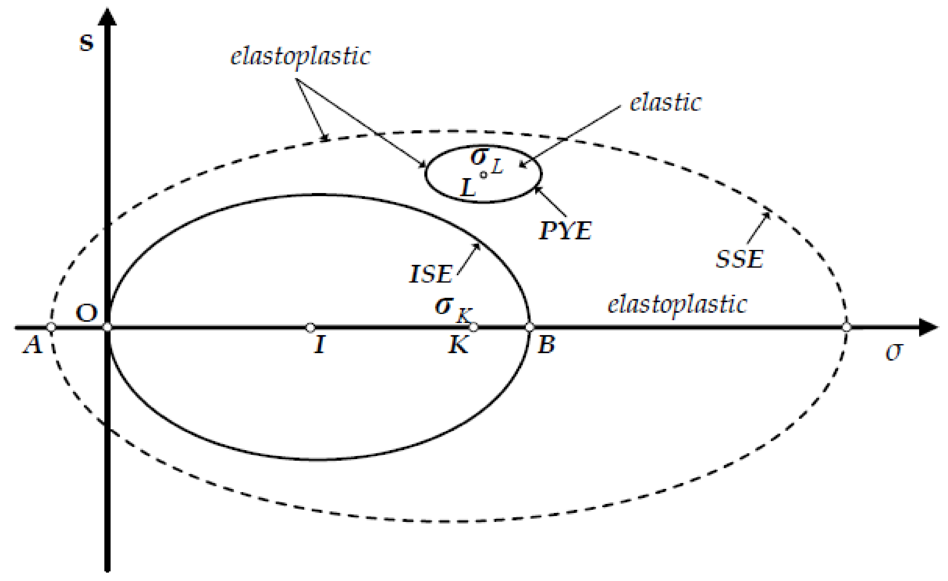
3.1. Plastic Yield Envelope and Bond Strength Envelope Mathematical Representation

The material yield function used in this paper is a modified Cam Clay type model. In this section the effective stresses in the solid skeleton are considered. The model is defined by two surfaces, the plastic yield envelope (PYE) which defines the elastic region and the bond strength envelope (BSE) which defines the acceptable positions for PYE [31,32,44,45,46]. BSE is influenced by the structure of the cohesive soil microtiles. If a stress point lays in the BSE boundary, the structure degradation rate of the clayey soil is maximized. Both envelopes are ellipses and are depicted in Figure 1.
The general representation of an envelope is the following:
f g ( p h , s , p L , s L , a ) = 1 c 2 ( s s L ) : ( s s L ) + ( p h p L ) 2 ( ξ a ) 2 = 0
In Equation (6) the general stress point σ has a hydrostatic component p h and a deviatoric component s while the centre of the ellipse L has a hydrostatic component p L and a deviatoric component s L . Moreover, a is the halfsize of the large diameter of BSE and a similarity factor ξ in introduced. When the deviatoric part of the centre of the ellipse is not zero and the hydrostatic part is not equal to a then the generalized envelope coincides with the plastic yield envelope of the stress point.
f g ( p h , s , p L , s L , a ) = f p ( p h , s , p L , s L , a )
However, if s L = 0 , p L = a then ξ = 1 and consequently the bond strength envelope is obtained:
f g ( p h , s , p L , s L , a ) = F ( p h , s , a ) = 1 c 2 s : s + ( p h a ) 2 a 2 = 0
For the simulation of the elastic behaviour the integration point is assumed to be poroelastic. The bulk modulus, proportional to the shear modulus as a consequence of a constant Poisson ratio, is as follows:
K b u l k = ν p h κ
ν denotes the specific volume of the soil.
The aforementioned material constitutive model is reliable for the majority of natural cohesive soils, of which the friction angle varies between 17 and 30 . The representation of the response of a clayey soil point is accurate in all possible loadings. Moreover, the equations of the criterion are in closed form which contributes to a stable numerical system. In addition, when large values of OCR of a cohesive soil is simulated this yield function can be easily reformed to take into account possible tensile stresses. The stresses and the strains algebraic transformations are performed in order to have energy conjugate amounts by adopting the numerical transformations used in Von Mises yield criterion. In this context the following variables are introduced
q = 3 / 2 s : s , e = 2 / 3 ϵ dev : ϵ dev
The variable e is used for denoting deviatoric strain measure whilst q is used for denoting the deviatoric stress measure (Von Mises stress).

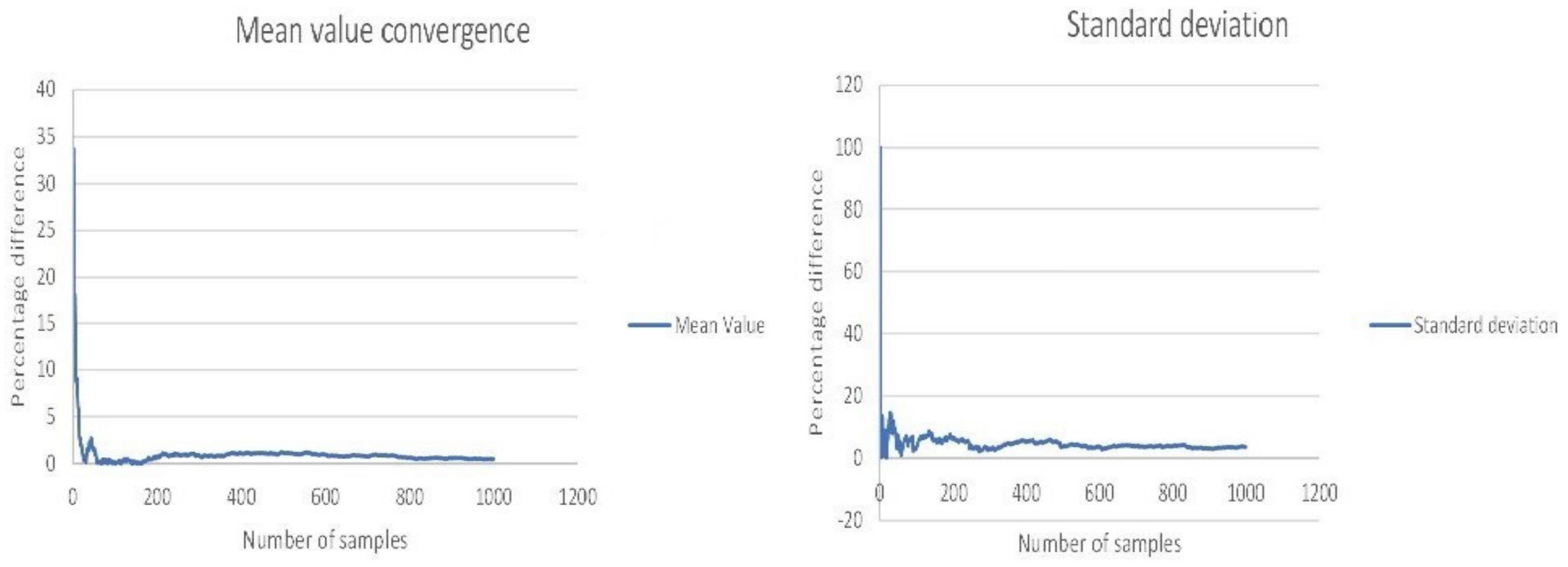
4. Stochastic Processes, the Truncated Normal Distribution and Latin Hypercube Sampling

4.1. The Karhunen–Loeve Series and the Truncated Normal Variables

The material uncertainty of the random parameters can be interpreted either by considering that the nodal points following random variables with deterministic shape functions, or by using the Karhunen–Loeve series expansion for the estimation of a realization of a random field [47,48,49,50,51,52,53]. In this paper, both methods are used in order to evaluate the performance of each simulation procedure.
The method of the Karhunen–Loeve series expansion applied in the present work, is formed for the calculation of H 1 ( x , ω ) , a random field of mean μ ( x ) based on the exponential autocovariance function. Denoting with b the correlation length the autocovariance function is stated as:
C h ( x 1 , x 2 ) = σ d 2 e x 1 x 2 b
A realization H 1 of the field considering M e number of eigenfunctions ϕ i with corresponding eigenvalues λ i can be computed as:
H 1 ( x , ω ) = μ ( x ) + i = 1 M e λ i ϕ i ( x T p ) ξ i ( ω )
where ξ i is a set of random variables of zero mean and covariance function C O V ( ξ i , ξ j ) = δ i j and T p is the symmetrization factor of the subspace of the process. If a stochastic process is Gaussian, as adopted in this paper, the ξ i functions are a set of standard normal random variables. This series expansion is the most widely used due to its high accuracy. If the Fredholm eigenvalue problem cannot have an analytical solution, and this takes place when the autocovariance function is more complicated, numerical methods can be introduced [19,50].
In [47] a method for interpreting the spatial randomness of a material parameter has been proposed, in which the random function f is formed with the implementation of shape functions N i . Denoting with f i the nodal point values, which are random variables following a probability density function (PDF) and N 0 the total number of shape functions the random function f takes the form:
f ( x ) = i = 1 N 0 N i ( x ) f i
In the present work, linear shape functions are adopted and the f i follow the truncated normal distribution ([39,40,54,55]), whose PDF is described by the equation
h 1 ( x ) = ϕ ( X 0 ) σ d ( Φ ( B ) Φ ( A ) )
In Equation (14), A, B, X 0 denote the normalized coordinates of the subspace limits and x, respectively while ϕ ( X 0 ) and Φ ( X 0 ) denote the standard normal probability and cumulative distribution function for X 0 . Additionally, σ d and the mean value of the normalization corresponds to the PDF of the random variable before truncation.

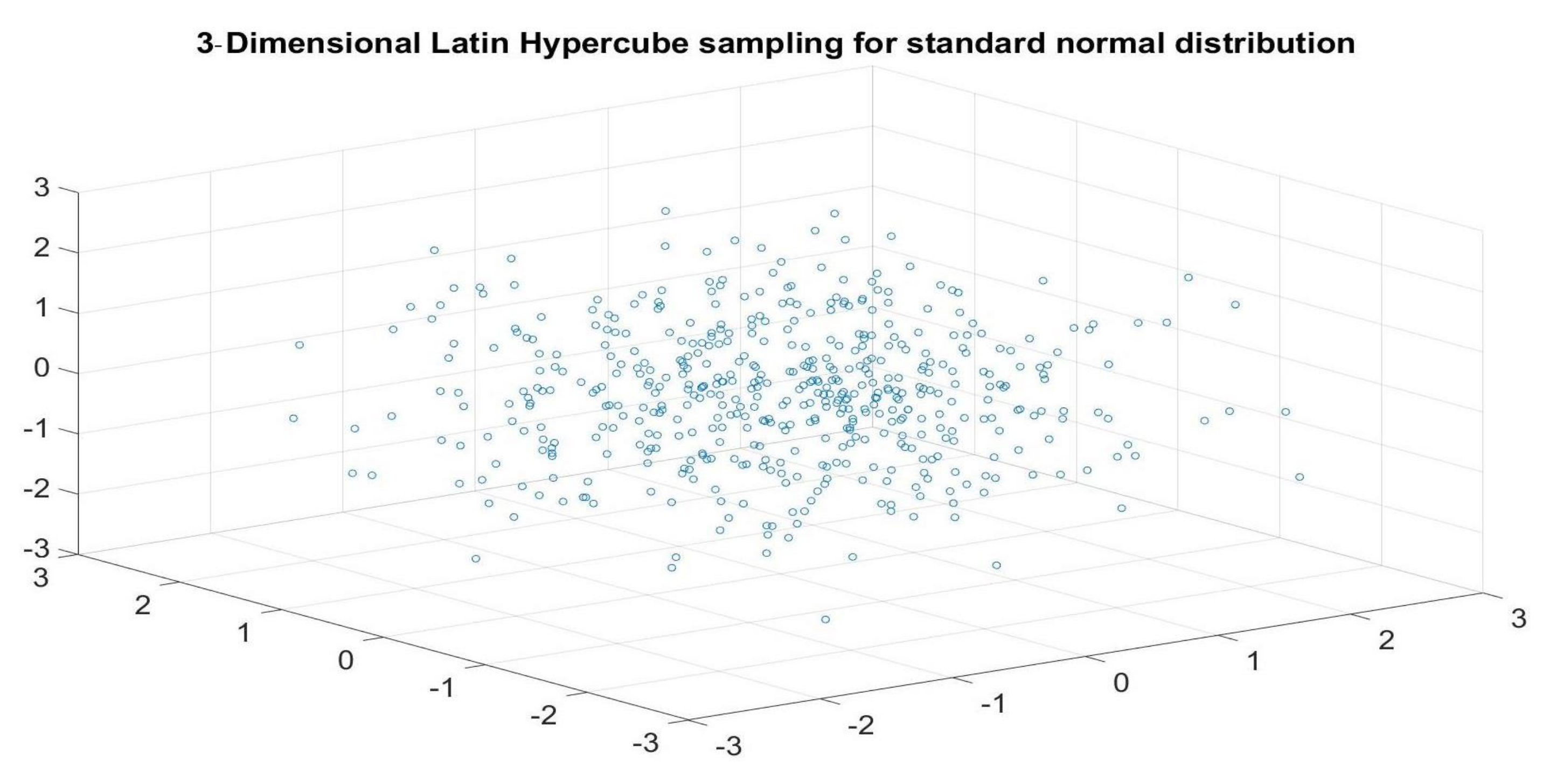
4.2. Latin Hypercube Sampling

The random vector samples can be selected by implementing pseudorandom unbiased algorithms to generate a large random vector, or by variance reduction methods like importance sampling [56] and Latin hypercube sampling (LHS) ([26,27]). The choice of the random vector through LHS the method reduces notably the computational cost in order to estimate the statistical moments of the output random variables.
The Latin hypercube procedure is as follows: consider X as a random vector ( x 1 , x 2 ,... x n ). For each random variable x i the following are made:
  • The interval [0,1] of the cumulative distribution function (CDF) is subdivided into N s equal subspaces
  • A random number is chosen and through the inverse CDF a sample x i is acquired
  • All the x i vectors are permuted in a random way and thus the vector realization X is composed
The aforementioned procedure ensures that at each possible row and each possible column in the (n x n) Euclidean space one sample is exactly extracted. This attribute is portrayed in Figure 2.
The most profound advantage of this scheme is that a smaller amount of values in comparison with the crude Monte Carlo simulation are required to integrate the PDF of the input uncertainty and subsequently to approximate the variability of the output. Moreover, the subintervals in each dimension are of different sizes in order to take into consideration possible asymmetries of the PDF of the input. This perspective can be used to cross-correlate variables, i.e., when the correlation matrix is not diagonal, thus it is of general application in the uncertainty quantification in engineering systems. In the present work the variables are not cross-correlated and the LHS sampling is implemented to acquire samples for the variables in the 3-dimensional space of the compressibility factor κ , the critical state line inclination c and the permeability k.
The material random variables following the PDF h 1 of Section 4.1 and the random field realizations calculated with the Equation (12) effect the finite element numerical scheme of Equation (1). The corresponding matrices C , K and F alter due to the randomness of the compressibility factor κ , as well as of the critical state line inclination c and the permeability k. The selection of the samples follows the importance sampling technique of the LHS method.

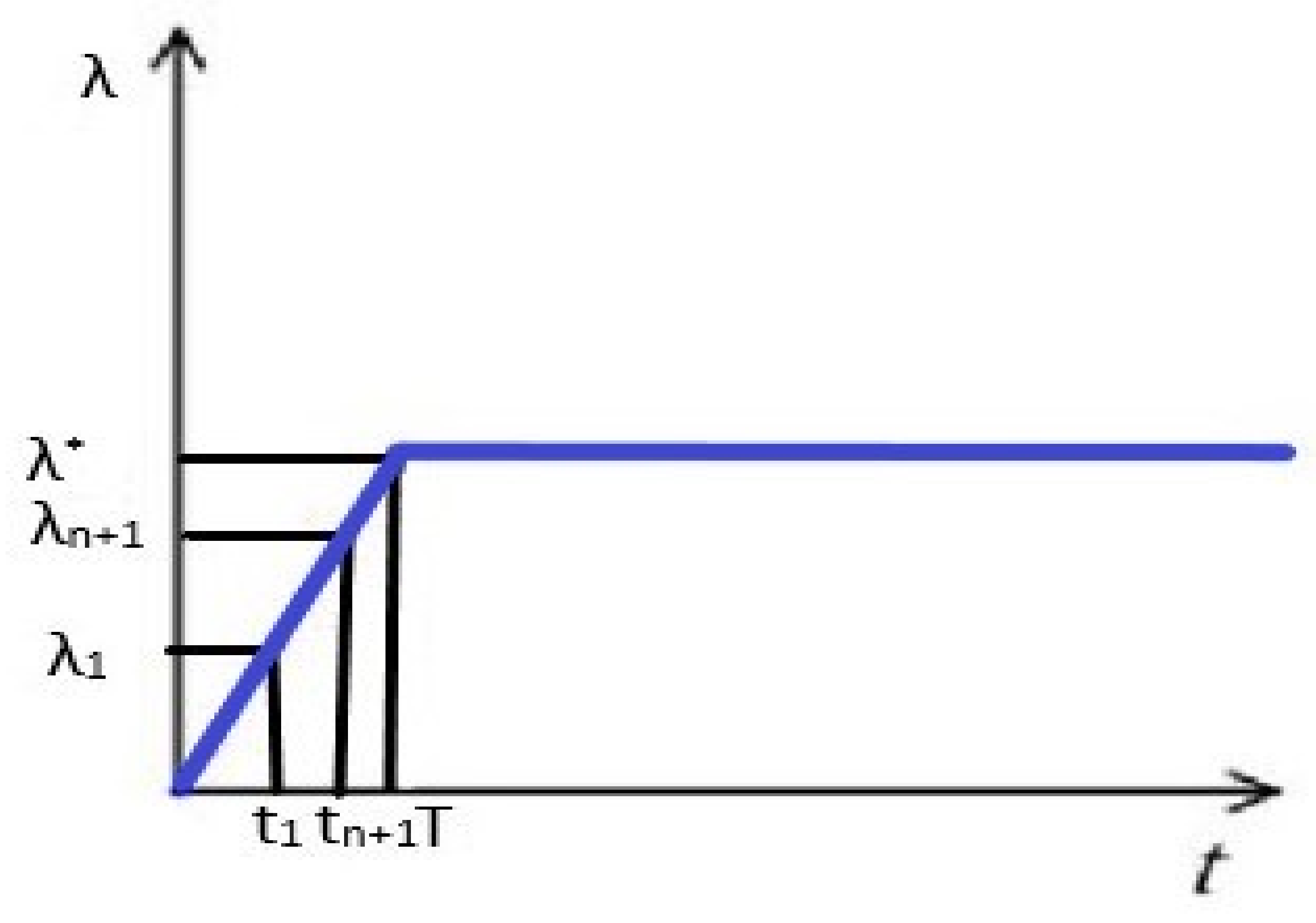
5. An Improvement of a Proposed Algorithm for the Determination of Failure Load in Ramp Dynamic Load Function

In this section an improvement of an algorithm proposed by the authors of [35] for the determination of failure load, when the dynamic loading function is the ramp loading function, is presented. The aim of the algorithm is to find the failure load at exactly the end of the ramp loading as indicated in Figure 3.
The objective of this algorithm is to estimate the load factor λ * which causes failure of a body at exactly the time T. An initial trial of λ 1 is considered leading to an initial time of failure t 1 is obtained. Then, for each new estimation λ n + 1 if the load factor λ n causes failure to the body is calculated by the equation
λ n + 1 = λ n t n T
If the load factor λ n is not causing failure, then the maximum no failure factor λ m a x n o f a i l u r e is acquired from all previous estimations used for the calculation of λ n + 1 , with the implementation of the following equation:
λ n + 1 = λ m a x n o f a i l u r e
In practice this recurrence relation usually converges ”by the failure region” which means that only Equation (15) is implemented. The difference between λ n + 1 and λ n is given by:
λ n + 1 λ n = λ n ( t n T 1 )
In Equation (17) it is evident that as n , t n T consequently, the left side of the equation tends to 0, and consequently the algorithm converges to the desired load factor λ * .
In Table 1 an investigation of the proposed algorithm is depicted. Comparing with the typical bisection method, where one should estimate initial values of failure and safety values λ 1 , f a i l and λ 1 , n o f a i l u r e and then compute the new load factor by the bisection of maximum safety factor and minimum failure factor, this algorithm gives less or an equal number of trials for the same initial failure guess and convergence tolerance, as is portrayed in Table 1. In addition, it needs only one initial guess, which makes the divergence of the solution less probable. In conclusion, as proven by the numerical tests presented in Table 1 and in Section 6, the divergence in failure load and failure displacement between the two algorithms is less than 1%. The absolute percentage difference is computed considering as exact solution of the bisection algorithm with an initial value of safety stress 1000 kPa. The computational performance for the 100 deterministic analyses of a Monte Carlo simulation is also presented in Table 1. The proposed algorithm can save up to almost 55% of the time demanded for a Monte Carlo analysis to be performed, indicating a considerable advantage of the aforementioned recurrence relation.

6. Numerical Tests on Stochastic Failure of Shallow Foundations with Random Linear and Non-Linear Material Properties

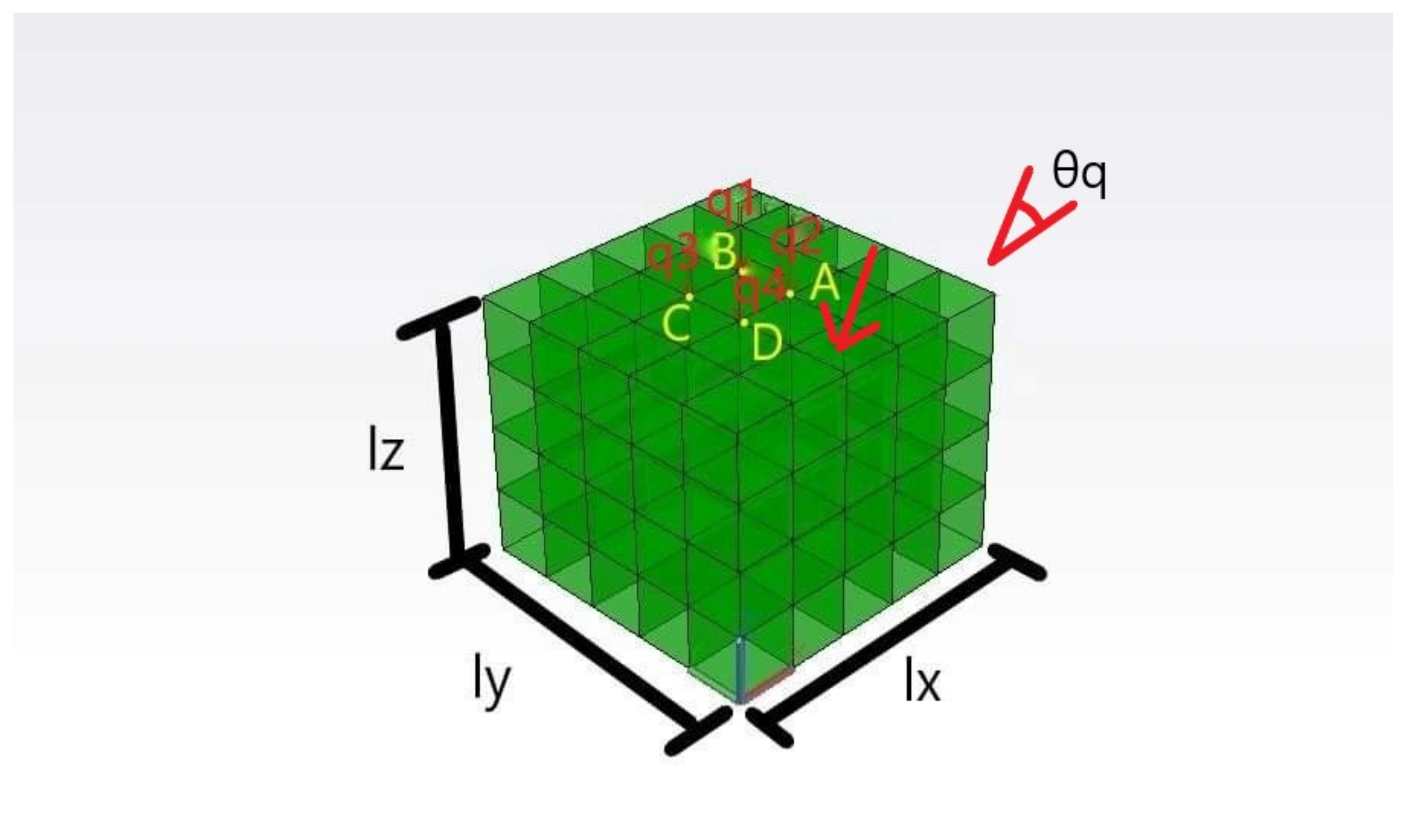
6.1. Description of the Problem

The proposed numerical simulation scheme is implemented in porous problems as portrayed in Figure 4 and are defined by the set of Equations (1). The monitored output variables are the total force of the footing settlement and its maximum and minimum displacements which are the mean value of displacements calculated at points A–D of Figure 4. The loading conditions consist of the oblique nodal values q 1 q 4 at points B, C, A and D respectively and incorporate the equivalent forces of an oblique shallow foundation load having angle of obliquity denoted as θ q , with respect to the horizontal direction and is uniformly distributed over the footing settlement surface. The modelling of the foundation consists solely of its equivalent forces along its surface ABCD, which is measured ( 1 × 1 m 2 ). The finite element mesh is constructed with eight node hexahedral finite elements with linear shape functions for u and p, which gives an acceptable numerical reliability [57,58]. The soil dimensions in X, Y, Z directions are respectively l x = 5 m, l y = 5 m, l z = 4 m. The geostatic stresses are directly imported as initial conditions, with the relations σ v = γ z , σ x = σ y = 100 kPa and are associated with stress point L of Figure 1. The simulation duration in all cases is one day and quasi static conditions are attained. A time step of dt = 0.001 d is adopted. The other deterministic parameters of the soil are given in Table 2.
In Table 2, λ denotes the inclination of isotropic compression line for the respective virgin normally consolidated clay and ν 0 denotes the initial specific volume of the soil, which is assumed proportional to κ . The boundary conditions are: u x ( z = h ) = u y ( z = h ) = u z ( z = h ) = 0 and the lateral boundary surfaces are constraint-free. The input material uncertainty consist of the material variables, the compressibility factor κ , the critical state line inclination c and the permeability factor k.
The compressibility factor κ , is considered as constant ( κ C ) over depth, or linear ( κ L ). In the κ L occasion, κ z = 0 = 0.008686 and the ratio R follows the truncated normal distribution with R = κ z = m a x κ z = 0 . The mean value of the ratio is μ R = 0.469 and the corresponding CoV is 0.25, as a consequence κ z = m a x , m e a n = 0.004074 . These values are chosen in order for the mean stiffness of the soil to correspond to a shear velocity of 200 m s . In Figure 5 the spatial distribution of κ L is portrayed. It should be emphasized that that bulk and the shear moduli are proportional since the Poisson ratio is assumed as constant. As a consequence, κ is directly related to the shear velocity. When κ has a constant distribution over depth, the mean value of κ is κ μ = 0.004074 and the CoV is 0.25.
For the critical state inclination c the constant variation over depth is presumed. Two possible considerations for the absolute value are implemented. If a random variable case is assumed c R , the friction angle ϕ 0 follows the truncated normal distribution with the mean value is μ ϕ = 23 and the standard deviation is σ ϕ = 2 which gives acceptable values for ϕ 0 considering for natural clays ([31]). A random vector of ϕ 0 is obtained through Latin hypercube sampling for the standard normal distribution. The vector ϕ 0 components are transformed into the truncated normal PDF h 1 . Finally, c is computed from c = 2 3 6 s i n ( ϕ 0 ) 3 s i n ( ϕ 0 ) . In an alternative case, for the deterministic value c D , c = 0.7336 for friction angle μ ϕ = 23 .
The permeability k, is considered constant over depth. The absolute value may be calculated by two possible cases. If a random variable approach is adopted k R , the mean value is μ k = 10 8 and the CoV is C o V k = 0 , 25 . On the other hand, for the deterministic case k D , k = 10 8 .
Two types of analyses are investigated. The solid analyses, where the water flow is not taken into account and the porous analyses, where the pore pressure is considered. The solid analyses performed, denoted with ( S ), are presented in Table 3, using linear (L) or constant (C) distribution for κ and deterministic (D) or random variable (R) cases for c. The corresponding porous analyses performed abbreviated are depicted in Table 4, incorporating linear (L), constant (C) and random field (RF) distribution for κ . Deterministic (D), random variable case (R) and random field (RF) distribution for c. Deterministic (D), random variable case (R) and random field distribution (RF) for k.
In the stochastic processes the mean values are chosen as follows: κ m e a n = 0.008686 , c m e a n =0.7336 and k m e a n = 10 8 m 3 s M g r following [41,43,59]. The standard deviations chosen are: σ κ = 0 , 25 κ m e a n , σ ϕ = 2 and σ k = 0 , 25 k m e a n . The exponential autocorrelation function described in Section 4.1 is used in all stochastic processes. The correlation lengths are chosen b = 2 m ( k R F ), b = 4 m ( k R F ) and b = 8 m ( k R F ). The spatial distributions for κ , κ L and κ C , as well as the random variable distributions for all material variables are a random variable case analysis. For c a constant deterministic analysis is assumed. The random field (RF) distributions refer to the Karhunen–Loeve series expansion and realizations of the spatial stochastic process are computed through equation H 1 of Section 4.1 with the use of the autocovariance function given by Equation (11).
The simulations are static, and the number of Fredholm eigenfunctions taken into account is eight. Failure is defined when the first Gaussian point exhibits softening behaviour (i.e., plastic hardening modulus H < 0). Each Monte Carlo simulation was implemented with 100 samples, using the Latin hypercube sampling method, which led to convergence for the mean value and standard deviation of the monitored displacements as depicted in Figure 6 where 1000 samples were taken for a randomly selected Monte Carlo simulation and compared to the corresponding statistics for 100 samples. It should be mentioned that the cross-correlation of all material variables is not taken into account and subsequently the correlation matrix is diagonal.

6.2. Presentation of the Results

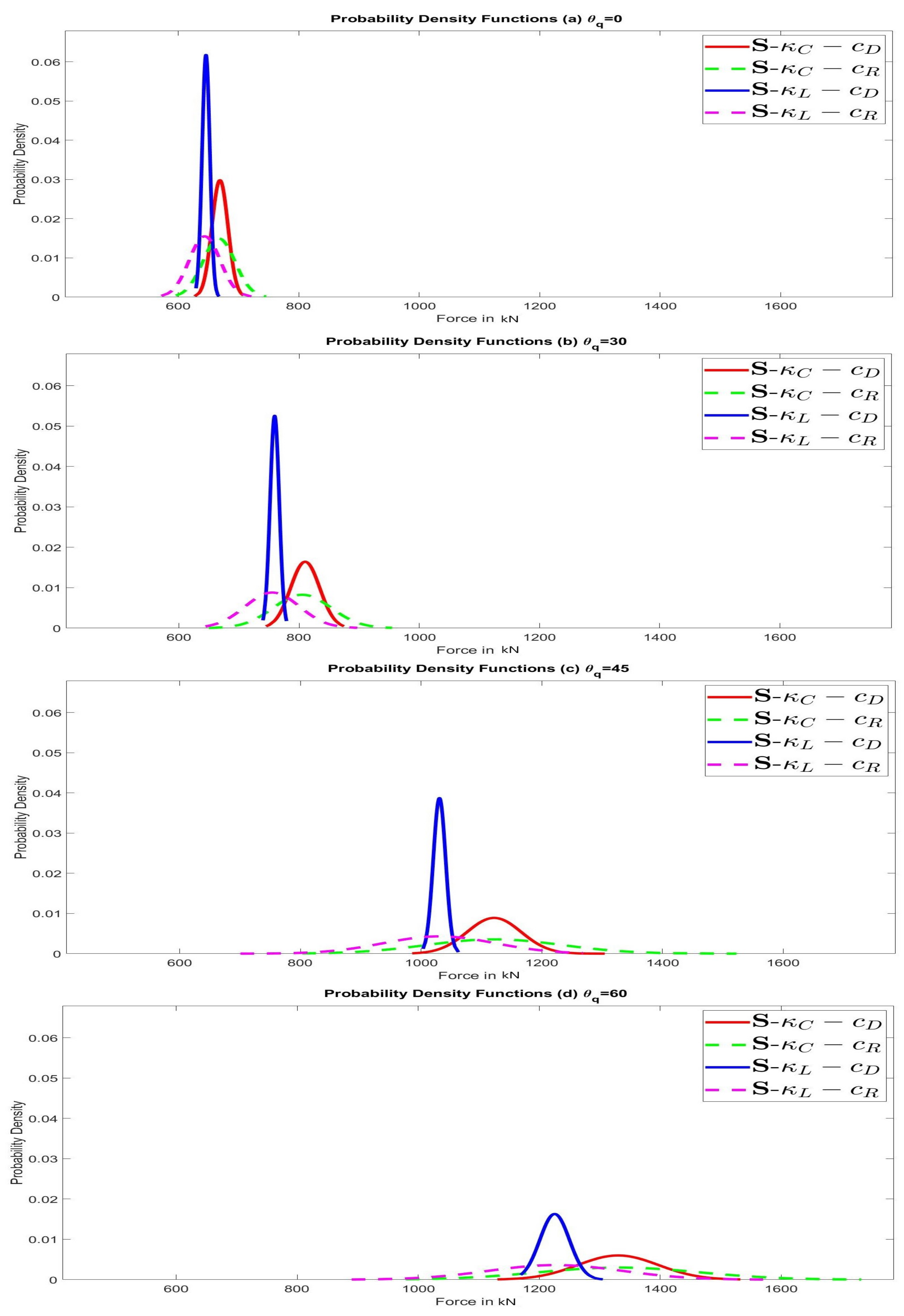
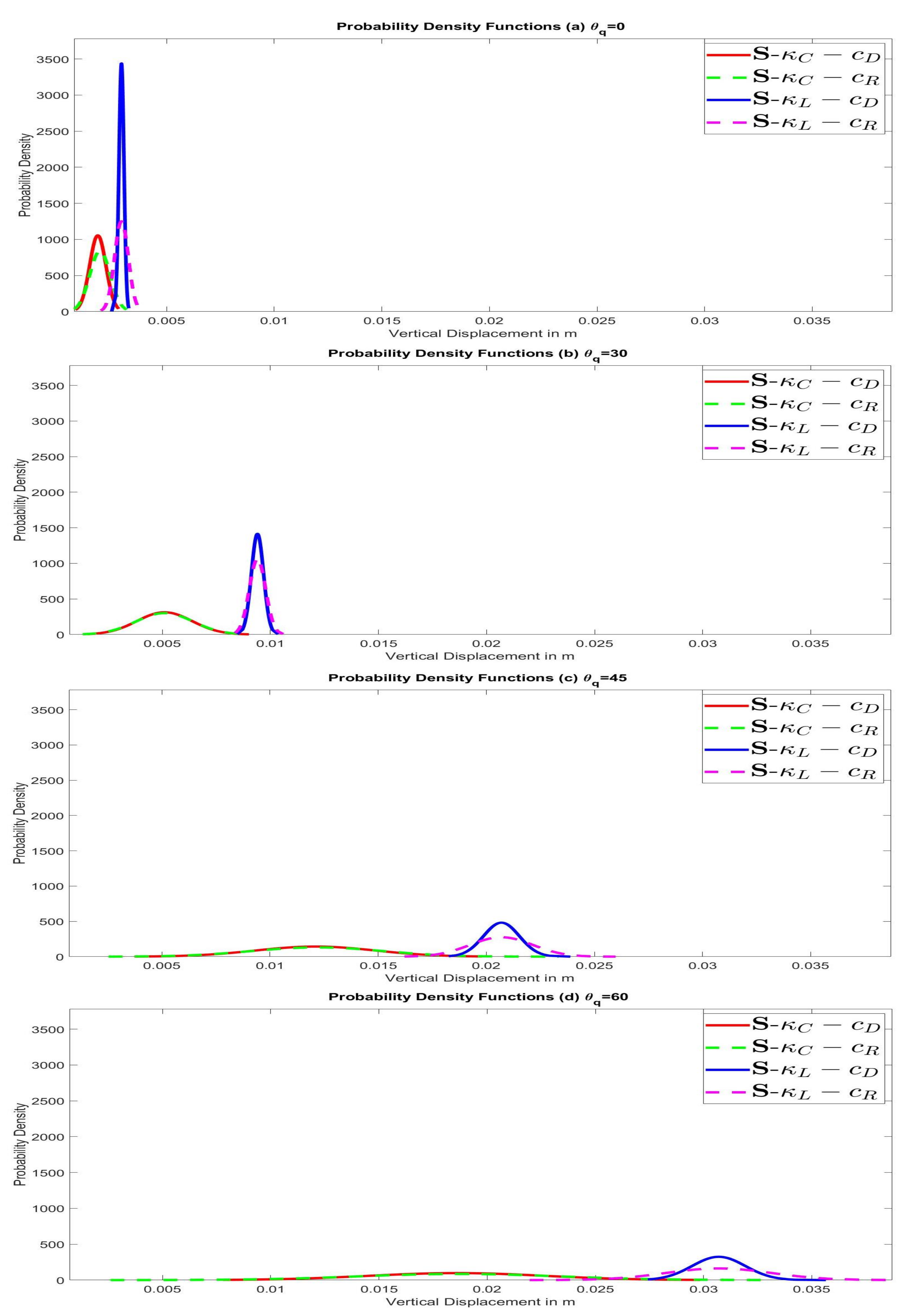
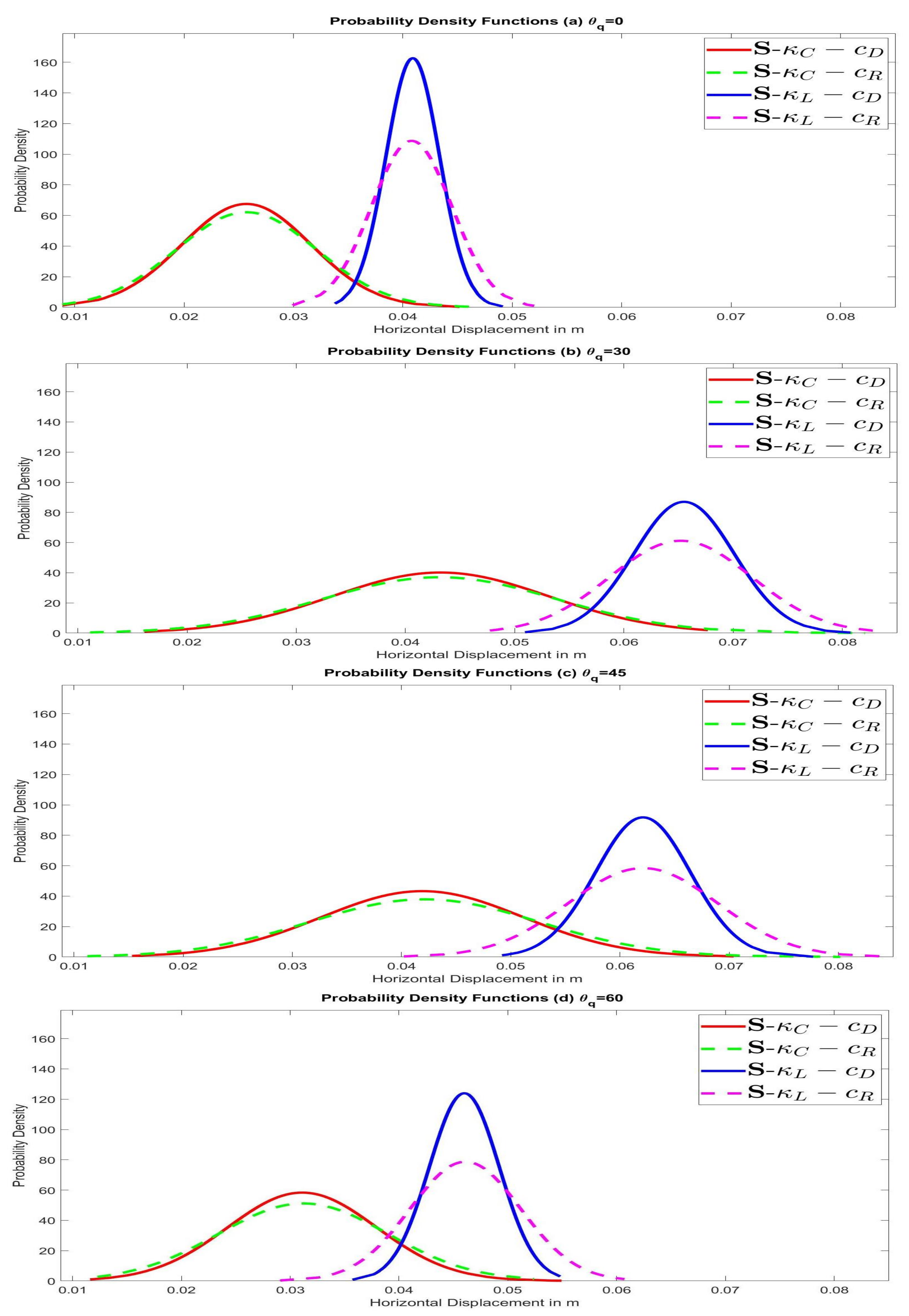
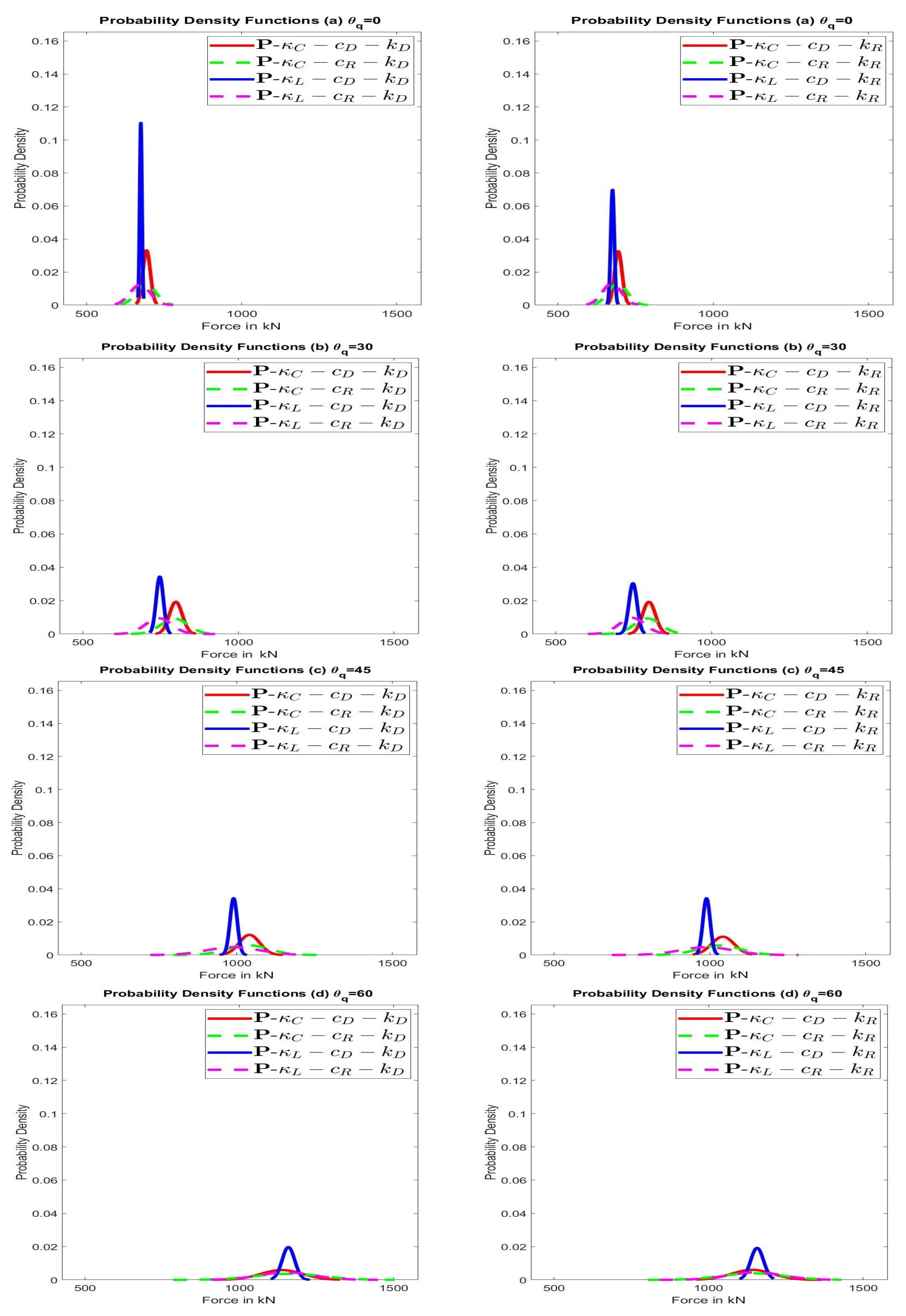
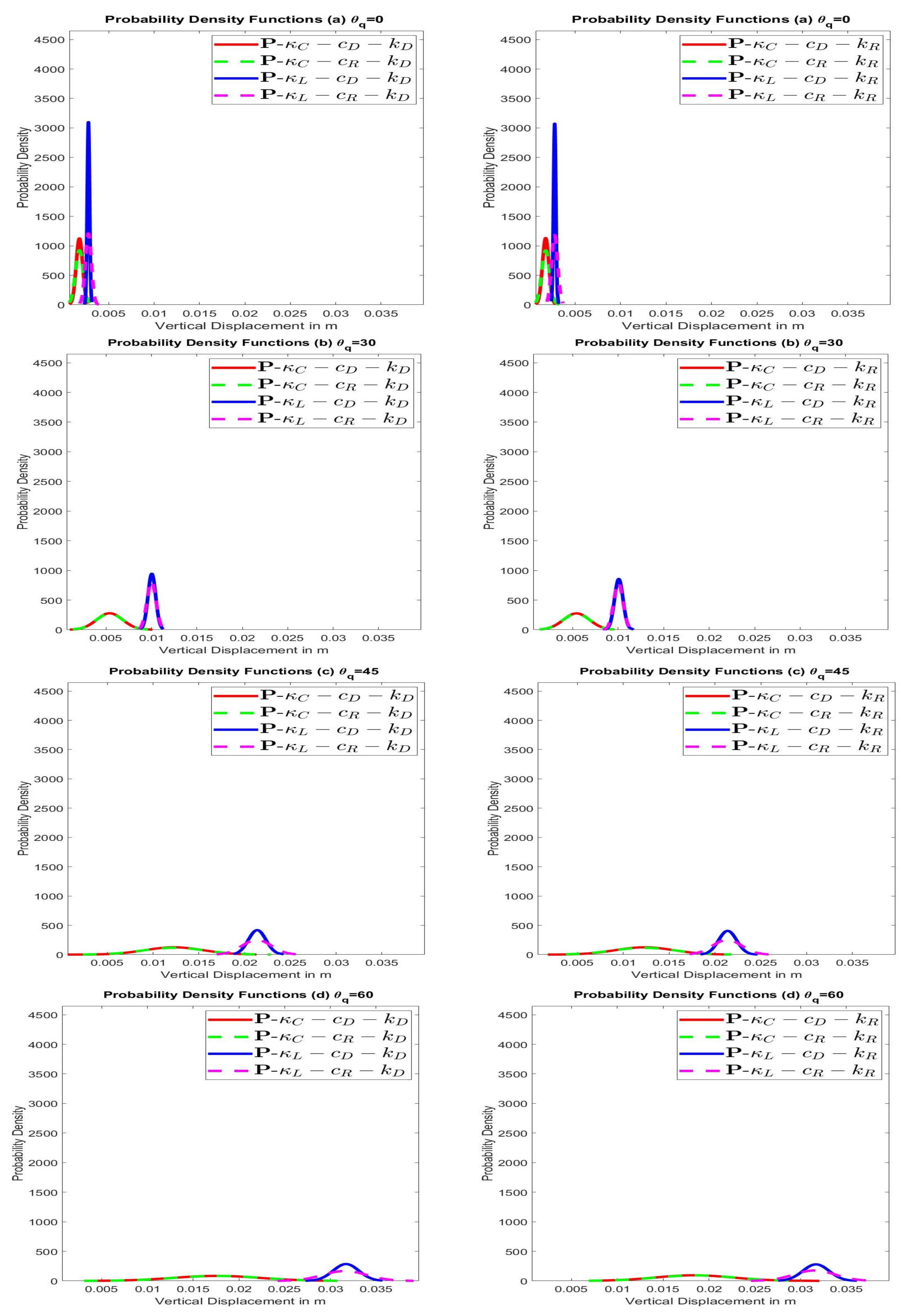
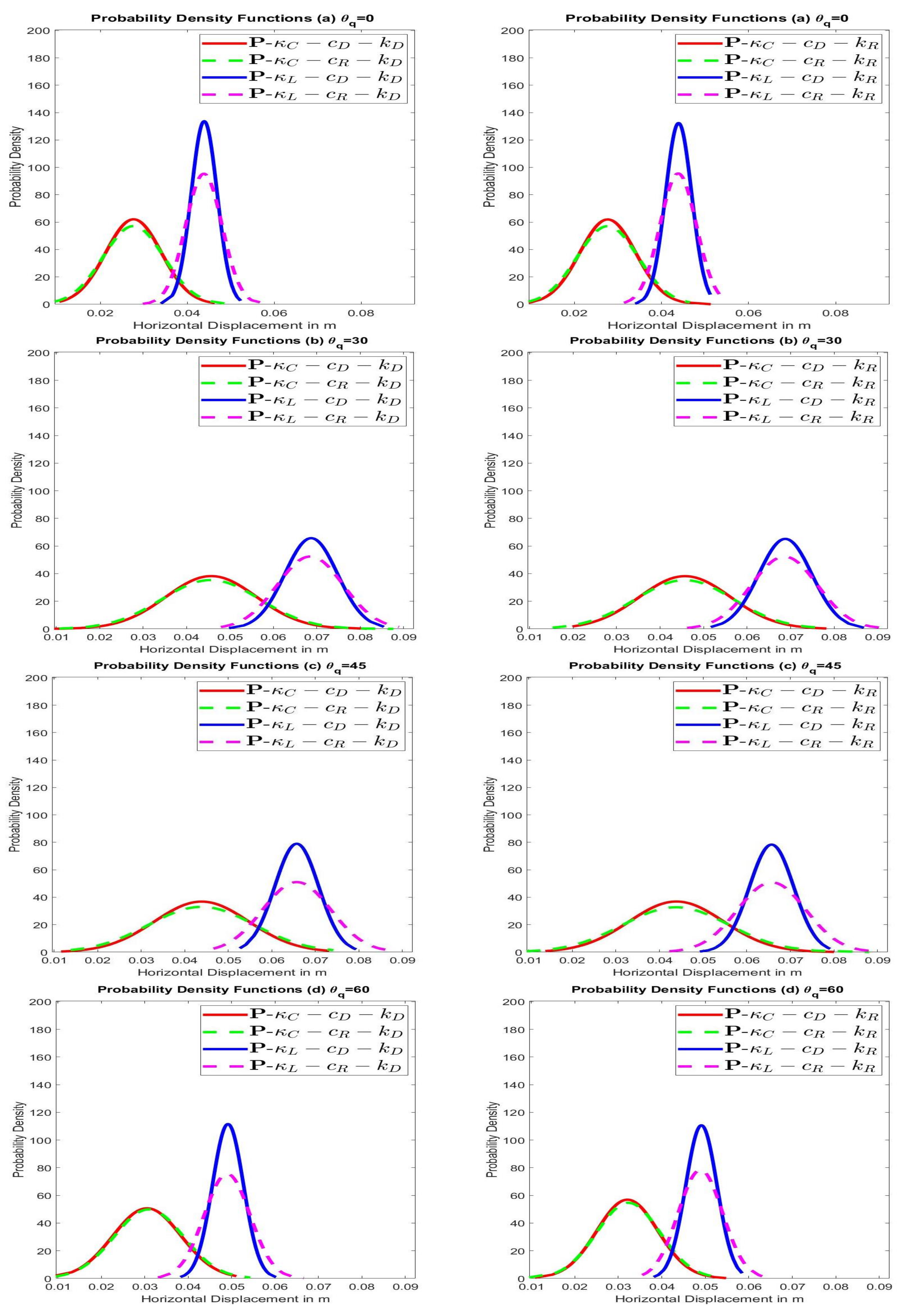
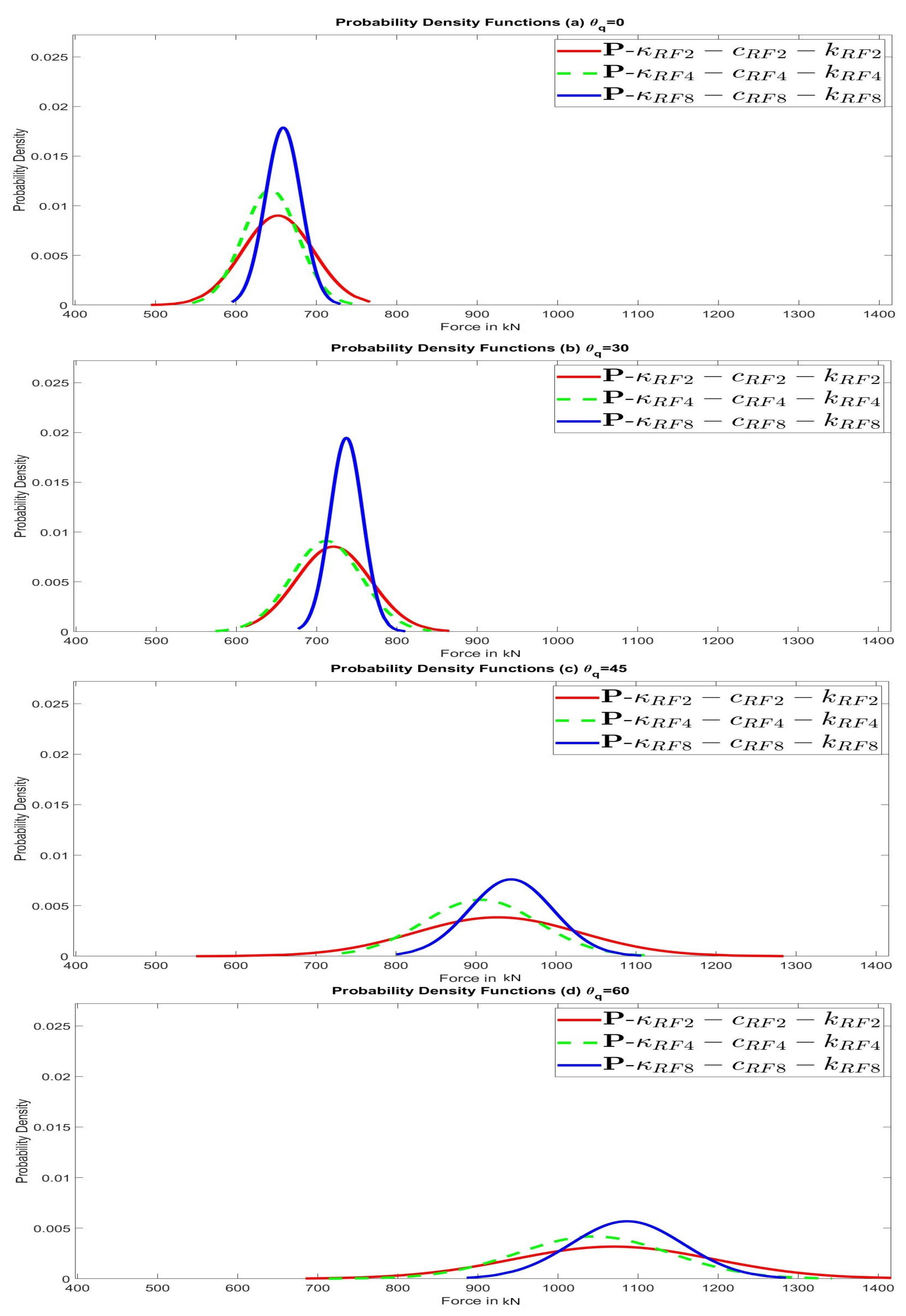
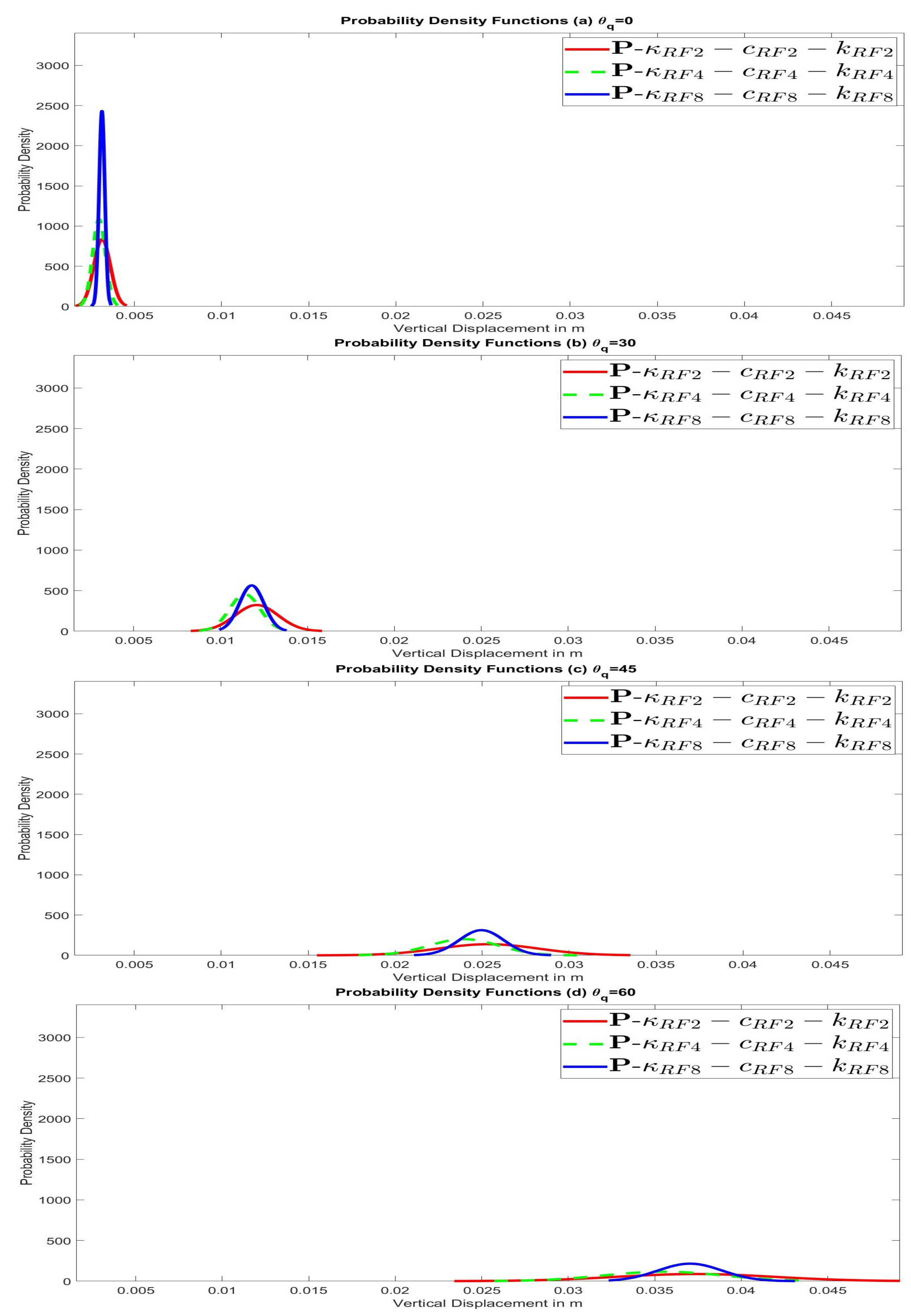
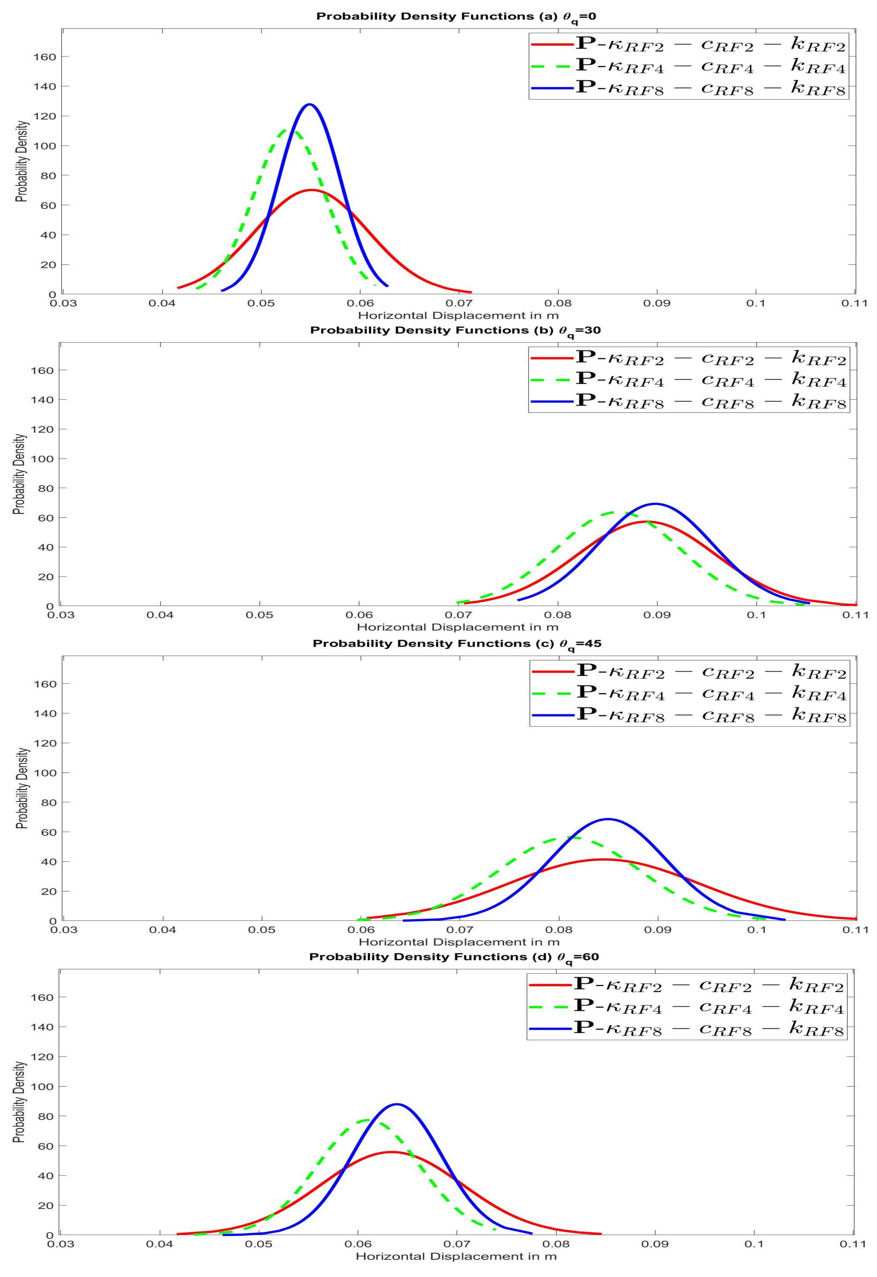
6.2.1. Limit Failure Force and Displacement

The results for the statistics of failure force and failure displacement are presented in Table A1, Table A2 and Table A3 and in Figure A1, Figure A2, Figure A3, Figure A4, Figure A5, Figure A6, Figure A7, Figure A8 and Figure A9 in Appendix A. In these tables the mean values ( μ ν ) of the total settlement force N, the vertical displacement u y and the horizontal displacement u x at failure are portrayed with the coefficient of variation (CoV) ( σ δ ) as well as the maximum (M) and minimum μ values acquired from the Monte Carlo simulation. The PDFs of the simulations are portrayed in the presented figures. They have been obtained by implementing the Kolomogorov–Smirnov test for proving their Gaussian normal distribution and then the corresponding histograms are smoothened for drawing the probability density function.
As portrayed in Table A1, when the water flow is not present, larger mean failure displacements and lower CoV are obtained when κ L is assumed compared to κ C . In addition, a smaller mean total foundation load is obtained when κ L case is adopted whilst the corresponding uncertainty is maximized for the κ c c R case. In solid analyses the maximum CoV of the output for failure footing force is 40% the input variability while the largest CoV for failure displacement in both directions is the same as the input uncertainty (see κ C c R for all monitored variables). This applies for all values of obliquity angle θ q . The mean value of N for θ q = 60 degrees is 1,9 times than the value for θ q = 0 . The mean values for the u y increase with the increase of θ q while for u x the critical angle for the maximization of its mean value is θ q = 30 . Thus, the critical spatial distribution of κ for the CoV of the output in all monitored variables is the κ C case and for c, the random variable case. The PDFs of solid analyses are portrayed in Figure A1, Figure A2 and Figure A3 where it can be concluded that the increase of obliquity leads to an increase of N and u y while for u x for obliquity angles of more than 30 degrees, a significant decrease is observed. This behaviour in the displacements is explained by the fact that in κ L distribution the upper compressible layers of the soil, have smaller CoV of κ causing smaller variability for displacements and strains. The assumption of constant variation over depth of the soil mass tends to be more homogeneous and stiff and, consequently the Gauss points have greater stiffness and larger failure footing forces occur.
The output uncertainty of the foundation total load in porous analyses is influenced to the same magnitude compared to solid problems with the alteration of obliquity. The variability of the output failure displacements increases with the increase of the obliquity until the angle of 45 degrees and then decreases, unlike the corresponding solid analyses in which the obliquity has practically no influence on the CoV of the output. As depicted in Table A2, the largest CoV of the footing total load, which is found at P κ C c R k d , θ q = 60 , is 40% of the variability of the input, while for both horizontal and vertical displacements the maximum CoV is 12% greater than the uncertainty of the input and is located at P κ C c R k d , θ q = 45 . Therefore, when taking into account the pore pressure in the soil domain, a decrease of the variability of the failure footing force takes place whilst in failure displacements when there is constant variation over depth for κ , a significant uncertainty enlargement occurs, as indicated in Figure A4, Figure A5 and Figure A6. This way of behaving can be attributed to the fact that when a constant spatial variation of a material variable is adopted, all Gauss points are associated with greater uncertainty leading to larger CoV for strains and displacements. Taking into account that the bulk modulus is related through Equation (9), in porous problems it is generally smaller than the corresponding solid problems, it is concluded that smaller mean values of failure force and smaller variability are expected, due to tensile failure of the first Gauss point. This will be proven numerically in Section 6.2.2 in Table A4, Table A5 and Table A6.
Porous analyses with the assumption that the material variables follow a stochastic process are conducted as a more general case in order to take into account the spatial randomness of the material parameters of the soil. In porous random field simulations, the greatest CoV of the shallow foundation total load is 48% the input uncertainty, while for the displacements the reduction of the variability is by 40% and 56% for the vertical and horizontal displacement, respectively. As depicted in Table A3, the critical correlation length for maximizing the output uncertainty is b = 2 m whilst for minimizing the mean foundation force is b = 4 m for all obliquities examined. When b = 2 m, the vertical mean failure displacements are the largest whilst for mean horizontal displacements for θ q = 0 the critical value for b = 2 m and when θ q > 0 the corresponding critical failure displacements occur when b = 8 m. The mean values of failure total foundation force in porous random field analyses are slightly smaller, with divergence on the vicinity of 10% compared to porous analyses with deterministic shape functions for the material parameters κ , c, k while the mean values for the failure displacements in both horizontal and vertical directions are larger in the porous analyses with random field representation for all the material variables. In the vertical displacements the enlargement compared to the corresponding porous analyses with deterministic shape functions for κ , c, k is in the order of magnitude of 20% whilst in the horizontal displacements it is in the vicinity of 30%. The unfavourable situation takes place when the foundation force is small and, consequently, the critical spatial distribution for the mean value of N is the random Karhunen–Loeve expansion for all material input variables and b = 4 m. The probability density functions of P - κ R F - c R F - k R F are portrayed in Figure A7, Figure A8 and Figure A9.
The results acquired give qualitative statements and quantitative proposals on the influence of the input uncertainty of each material variable in porous failure phenomena taking into account the obliquity of the shallow foundation. The compressibility factor κ affects the statistical moments of all monitored variables. This effect in CoV of the output is more profound when κ is uniformly distributed along the depth. This holds in both porous and non-porous problems which can be attributed to the fact that κ is directly associated with the bulk modulus and consequently this reflects on the strains the displacements and the stiffness of the soil domain leading to larger alteration of the footing force.
The permeability k has alleviated the effect of failure shallow foundation forces and failure displacements. The spatial variability of k appears to influence to a lesser extent the CoV of the output in most Monte Carlo analyses. For porous consolidation problem with the load geometry and deterministic parameters remaining the same, the output displacements and stresses field are not influenced by the permeability since the pore pressures are fully dissipated, as verified by the numerical results.
Finally, the uncertainty of a plastic variable like the critical state line inclination c of the material model appears to have the most notable effect on the uncertainty of the shallow foundation total load and the corresponding displacements when the constant variation over depth and random variable case c R is adopted. The mean values for failure force are critical when c R case is assumed. For mean failure displacements the alteration of c has a negligible effect in all obliquities in both solid and porous problems. This can be explained by the fact that c is directly influenced by the integration point state at failure, subsequently it alters the limit load of the soil domain.
The validity of the PDFs presented has been verified in two ways. Firstly, the histograms obtained from each Monte Carlo simulation are smoothed and the aforementioned curve is estimated as a Gaussian normal PDF or a Gaussian lognormal PDF respectively. The Gaussian lognormal PDF is estimated when the CoV is large. Subsequently, the Kolomogorov and Smirnov test for the numerical validation of this assumption is performed. In all cases the null hypothesis for the 5% reliability interval is accepted so in all cases either the normal PDF or the lognormal PDF is thpropriate for the output monitored variables. In the present work since the largest CoV of the output obtained provide a small probability of negative values for the monitored output variables, the normal probability density functions are assumed.

6.2.2. Limit Stresses–Strains and Failure Spline

The results for the limit stress–strain statistics and failure splines are portrayed in Table A4, Table A5 and Table A6. In these tables the following statistics are given: mean values, CoV and minimum values for the volumetric stresses denoted as p v o l , and deviatoric Von Mises stresses denoted as q d e v , as explained in Section 3.1. Moreover, the mean value with the CoV of the volumetric strains denoted as e v o l and the deviatoric strains denoted as e d e v are also presented in Table A4, Table A5 and Table A6, The probability of first Gauss point failure for all simulations is also depicted. At this point, it is declared that the volumetric strain at failure is tensile.
As depicted in analyses of non-porous medium of Table A4, larger uncertainty of the output and reduced minimum value of failure volumetric and deviatoric stresses are acquired when c R case is assumed. This assumption for critical state line inclination give the greatest variability of the strains at failure in all obliquities. The mean value for the volumetric component is in the vicinity of 15‰ for the linear variation over depth for κ and in the vicinity of 7‰ for the constant variation over depth for κ . The respective values for the deviatoric component are 18‰ and 10‰. From the output results of the Monte Carlo simulation it can be concluded that the percentage of plastic deviatoric strains are larger when θ q = 0.30 , thus the distortional failure is critical. For θ q = 45.60 the volumetric failure is evident. Finally, when the obliquity is not present, which means when pure horizontal loading is applied, (3.21, 2.21, 3.79) is the critical integration point, whilst when θ q > 0 , (1.79, 2.21, 3.79) is the critical Gauss point.
In porous simulations with deterministic spatial distributions for all the material parameters larger stress variability in both volumetric and deviatoric components is obtained when the κ L c R case is assumed, as portrayed in Table A5. The alteration of the permeability significantly affects the output uncertainty when θ q = 60 degrees in P κ C c R k D and P κ C c R k R analyses. The numerical Monte Carlo simulations indicate that the largest output uncertainty for volumetric strains is found at θ q = 60 , P κ C c R k R while for deviatoric stresses is located at P κ C c R k D for obliquity angle of 60 degrees. The mean value of volumetric strains varies between 5 and 8‰ and the mean values of deviatoric strains is in order of magnitude of 10‰, considering constant variation over depth for the compressibility factor. For κ L case the mean values are notably larger. From the output results attained it is evident that for small obliquities the volumetric failure is critical, while for larger angles, with the exception of θ q = 60 and P κ C c R k D case the distortional failure is evident. Finally, the most probable failure Gauss point is the (3.21, 2.21, 3.79) for θ q = 0 , (3.79, 2.21, 3.79) for θ q = 30 and (1.79, 2.21, 3.79) for θ q = 45 , 60 . As the obliquity increases more, integration points share a larger probability of failure. The smallest probability of the most profound integration point is over 80% indicating the importance of this Gauss point in the estimation of the failure spline.
In porous analyses with random process for κ , c, k, greater output uncertainty for stresses is obtained for b = 2 m, in all cases as portrayed in Table A6. The volumetric strains in most obliquities have critical correlation length b = 4 m and similar conclusions can be made for the deviatoric strains. Taking into account the numerical results obtained by the analyses simulated when b = 2 and θ q = 30 degrees the probability is divided to larger amount of integration points, consequently the variability of the failure mechanism is maximum. When the obliquity angle in degrees is θ q = 0.30 the volumetric failure occurs whilst if θ q = 45.60 the deviatoric failure takes place. Finally, when θ q = 0 the critical integration point is (3.21, 2.21, 3.79), when θ q = 30 the critical Gauss point is (3.79, 2.21, 3.79), when θ q = 45 , 60 the aforementioned spline point is (1.79, 2.21, 3.79).

7. Conclusions

In this paper, the variability estimation of the failure of shallow foundations on cohesive soils taking into account the pore pressure soil interaction with the use of the stochastic finite element method is depicted. The aim of this article is to provide a numerical tool for acquiring accurate quantitative results on the failure footing force and corresponding displacements in relation to the input variability of soil material parameters. The aforementioned numerical simulation model is valid for general assumptions for the geometry, the loading and the material distribution of the soil mass. In this context, a detailed finite element simulation, alongside an accurate and reliable material constitutive yield function are used.
The numerical results of the simulations portray that the monitored output variables of ultimate foundation load and corresponding displacements follow a Gaussian random distribution despite material non-linearity of high magnitude that is profound in failure phenomena. The randomness of material poroelasticity is important in the uncertainty of the output variables especially when it has a constant variation with respect to the depth of the soil domain. Analogous considerations can be made for the critical state line inclination c. When the constant distribution for κ is adopted, the CoV of the output maximum displacement is increased in relation to the input variability by 12%. The porous variable of permeability appears to have an alleviated influence to the uncertainty of the monitored variables. In porous problems the failure load when the obliquity is not 0, the mean failure foundation force is smaller in comparison with the corresponding non-porous medium.
The random fields for κ , c, k give larger mean failure volumetric and deviatoric strains for all obliquity angles examined. In porous stochastic process simulations when the load angle with respect to the horizontal direction is small, the volumetric failure is critical whilst when the obliquity angle is larger the distortional failure is critical. If deterministic shape function over depth is assumed for κ , c, k, similar conclusions can be made. In conclusion, when an a horizontal force is applied the (3.21, 2.21,3.79) is the most probable failure point and if obliquity is present the (1.79, 2.21,3.79) integration point is the most probable onset of the failure spline.

Author Contributions

Data curation, A.-A.S. and M.P.; Investigation, A.-A.S. and M.P.; Methodology, A.-A.S. and M.P. All authors have read and agreed to the published version of the manuscript.

Funding

This research received no external funding and the APC was waived by MDPI.

Institutional Review Board Statement

Not applicable.

Informed Consent Statement

Not applicable.

Data Availability Statement

Upon communication with the corresponding author.

Conflicts of Interest

The authors declare no conflict of interest.

Nomenclature

N f Friction variables
N q Friction variable indicating the influence of possible vertical load in the lateral of
the foundation
N c Friction variable indicating the influence of the cohesion of the soil
N γ Friction variable indicating the influence of the settlement dimensions
alongside with the total weight of the soil
S f Shape variables
S q Shape variable indicating the influence of possible vertical load in the lateral of
the foundation
S c Shape variable indicating the influence of the cohesion of the soil
S γ Shape variable indicating the influence of the settlement dimensions
alongside with the total weight of the soil
κ Compressibility factor
cCritical state line inclination
kPermeability in units m 3 s M g r
ϕ 0 Friction angle
M Total mass matrix
C Total damping matrix
K Total stiffness matrix
M s Solid skeleton mass matrix
ρ d Density of the soil
B Deformation matrix
E Elasticity matrix
C s Solid skeleton damping matrix
K s Solid skeleton stiffness matrix
m Unity matrix
b Loading vector
k Matrix of permeability in units m 3 s M g r
N P Shape functions for pore pressure
N u Shape functions for displacements
S Saturation matrix
Q c Coupling matrix
H Permeability matrix
f S Equivalent forces due to external loading
QVariable for combining the influence of bulk moduli of fluid and solid skeleton in
porous problems
σ Total stress tensor
s Deviatoric component of the stress tensor
p h Hydrostatic component of the stress tensor
aHalfsize of the bond strength envelope
s L Deviatoric component of the stress point of the centre of the plastic yield envelope
p L Hydrostatic component of the stress point of the centre of the plastic yield envelope
ξ Similarity factor between the plastic yield envelope and bond strength envelope
f g Generalized elliptic envelope
f p Plastic yield envelope (PYE)
FBond strength envelope (BSE)
ν Specific volume of the soil
qVon Mises stress
eDeviatoric strain measure
ϵ dev Deviatoric component of the strain tensor
fRandom function
f i Value of the random function at nodal points
N i Shape functions
N 0 Total number of shape functions
h 1 Truncated normal PDF
ϕ ( x ) Standard normal PDF
Φ ( x ) Standard normal CDF
σ d Standard deviation of the random variable before truncation
A, B, X 0 Normalized coordinates of the subspace of the truncated PDF
limits and x respectively
H 1 ( x , ω ) Karhunen–Loeve random field
N s Number of subintervals in the Latin hypercube Sampling
μ ( x ) Mean value of the random field
X ( x 1 , x 2 , x n ) Random vector created by the Latin hypercube sampling
M e , λ i , ϕ i Total number of eigenvalues λ i and eigenfunctions
ϕ i respectively
bCorrelation length
C O V ( ξ i , ξ j ) Covariance function
λ * Load factor causing failure of the body at exactly the time which ends
the rampload function
TTime which the rampload function ends
T p Symmetrization factor of the stochastic process
λ n Trial load factor of step n causing failure
t n Time of failure at the generalized load factor λ n
λ m a x n o f a i l u r e Maximum trial load factor which causes safety
λ 1 , f a i l Initial trial load factor causing failure
λ 1 , n o f a i l u r e Initial trial load factor which causes safety
q 1 q 4 Equivalent forces of the shallow foundation
θ q Obliquity angle
l x l y l z Dimensions of the total finite element mesh
σ v , σ x , σ y Geostatic stresses in vertical direction and directions x and y respectively
λ Inclination of isotropic compression line for the respective normally
consolidated clay
a i n i t i a l Initial halfisize of the ellipse
a r e s i d u a l Residual halfisize of the ellipse
OCROverconsolidation ratio
GShear modulus
K b u l k Bulk modulus
γ Specific weight
ν 0 Initial specific volume of the soil
u x Displacement vector in direction x
κ z = 0 
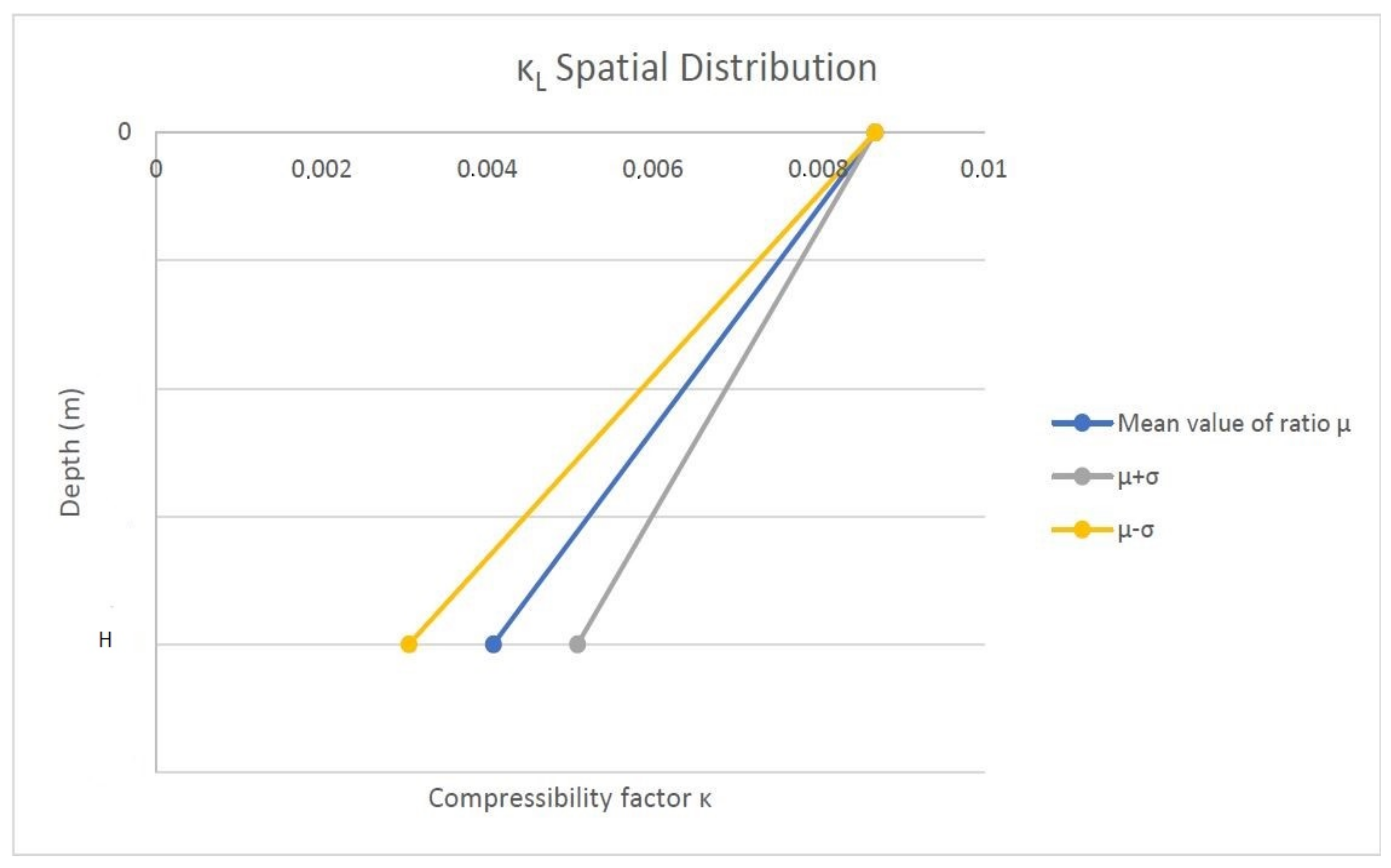
Compressibilty factor at depth = 0
κ z = m a x Compressibilty factor at maximum depth
R = κ z = m a x κ z = 0 Ratio of the compressibility factors measured at depth = 0 and at
maximum depth
μ R Mean value of ratio R
κ z = m a x , m e a n Compressibilty factor at maximum depth when the ratio R has its
mean value
κ L Linear distribution over depth for the compressibility factor
κ C Constant distribution over depth for the compressibility factor
κ μ Mean value of κ
c R Random variable case for the critical state line inclination
c D Deterministic case for the critical state line inclination
μ ϕ Mean value of the friction angle
σ ϕ Standard deviation of the friction angle
μ k Mean value of the permeability
C o V k Coefficient of variation of the friction angle
κ m e a n Mean value of the compressibility factor in the random field representation
c m e a n Mean value of the critical state line inclination in the random
field representation
k m e a n Mean value of the permeability in the random field representation
σ κ Standard deviation of the compressibility factor in the random field
representation
σ ϕ Standard deviation of the critical state line inclination in the random field
representation
σ k Standard deviation of the permeability in the random field representation
μ ν Mean values of the results
σ δ Coefficient of variation of the results
MMaximum values of the results
μ Minimum values of the results
NTotal settlement force
u x Horizontal displacement at failure
u y Vertical displacement at failure
p v o l Volumetric stress at failure
q d e v Von Mises stress at failure
e v o l Volumetric strain at failure
e d e v Deviatoric strain at failure
R v o l Percentage plastic volumetric strains at failure
R d e v Percentage plastic deviatoric strains at failure

Appendix A

The following tables and figures are placed in this section.
Table A1. Monte Carlo results for the settlement force (kN), the vertical and horizontal failure displacements (m) for non-porous medium ( θ q in degrees).
N θ q = 0 θ q = 30
S κ C - c D κ C - c R κ L - c D κ L - c R κ C - c D κ C - c R κ L - c D κ L - c R
μ ν 668.94667.19645.75643.56 809.81805.00759.06755.13
σ δ 0.020.040.010.04 0.030.060.010.06
M 700.00721.00658.00700.00 861.00882.00770.00833.00
μ 651.00609.00637.00588.00 777.00714.00756.00665.00
M μ 1.081.181.031.19 1.111.241.021.25
N θ q = 45 θ q = 60
S κ C - c D κ C - c R κ L - c D κ L - c R κ C - c D κ C - c R κ L - c D κ L - c R
μ ν 1120.901121.301030.301029.90 1330.401331.801225.401226.80
σ δ 0.040.100.010.09 0.050.100.020.09
M 1239.001358.001057.001218.00 1491.001624.001274.001456.00
μ 1043.00931.001008.00861.00 1232.001106.001190.001022.00
M μ 1.191.461.051.41 1.211.471.071.42
u y θ q = 0 θ q = 30
S κ C - c D κ C - c R κ L - c D κ L - c R κ C - c D κ C - c R κ L - c D κ L - c R
μ ν 0.00180.00190.00290.0029 0.00510.00510.00940.0094
σ δ 0.210.250.040.11 0.250.260.030.04
M 0.00260.00280.00310.0035 0.00750.00760.01010.0102
μ 0.00100.00100.00270.0024 0.00240.00240.00870.0088
M μ 2.672.731.161.44 3.163.181.151.16
u y θ q = 45 θ q = 60
S κ C - c D κ C - c R κ L - c D κ L - c R κ C - c D κ C - c R κ L - c D κ L - c R
μ ν 0.01210.01220.02070.0207 0.01860.01870.03070.0307
σ δ 0.230.250.040.07 0.220.250.040.08
M 0.01730.01820.02220.0233 0.02630.02780.03320.0352
μ 0.00600.00620.01880.0185 0.00950.00980.02780.0271
M μ 2.872.951.181.26 2.762.841.191.30
u x θ q = 0 θ q = 30
S κ C - c D κ C - c R κ L - c D κ L - c R κ C - c D κ C - c R κ L - c D κ L - c R
μ ν 0.02570.02570.04090.0408 0.04320.04310.06550.0652
σ δ 0.230.250.060.09 0.230.250.070.10
M 0.03700.03820.04540.0475 0.06170.06450.07450.0773
μ 0.01270.01300.03580.0362 0.02160.02200.05550.0563
M μ 2.912.941.271.31 2.862.931.341.37
u x θ q = 45 θ q = 60
S κ C - c D κ C - c R κ L - c D κ L - c R κ C - c D κ C - c R κ L - c D κ L - c R
μ ν 0.04190.04210.06210.0621 0.03110.03120.04600.0461
σ δ 0.220.250.070.11 0.220.250.070.11
M 0.05860.06320.07010.0749 0.04350.04650.05200.0554
μ 0.02160.02240.05250.0533 0.01610.01660.03900.0399
M μ 2.712.821.331.41 2.712.801.331.39
Figure A1. PDFs of the normal force of the settlement in kN for non-porous medium.
Geotechnics 01 00017 g0a1
Figure A2. PDFs of the vertical displacement in m for non-porous medium.
Geotechnics 01 00017 g0a2
Figure A3. PDFs of the horizontal displacement in m for non-porous medium.
Geotechnics 01 00017 g0a3
Table A2. Monte Carlo results for the settlement force (kN), the vertical and horizontal failure displacements (m) for porous analyses with linear and constant distribution for κ and c ( θ q in degrees).
N θ q = 0 , k D θ q = 0 , k R
P κ L - c D κ L - c R κ L - c D κ L - c R κ L - c D κ L - c R κ L - c D κ L - c R
μ ν 693.47691.40674.89672.91 694.26692.14675.75673.60
σ δ 0.020.050.010.05 0.020.040.010.05
M 724.10751.64683.38733.44 722.97751.66688.53733.60
μ 674.89629.52668.17607.46 675.09636.80665.44617.92
M μ 1.071.191.021.21 1.071.181.031.19
N θ q = 30 , k D θ q = 30 , k R
P κ L - c D κ L - c R κ L - c D κ L - c R κ L - c D κ L - c R κ L - c D κ L - c R
μ ν 798.42794.09746.87743.03 798.99794.52747.81744.16
σ δ 0.030.050.020.06 0.030.050.020.06
M 850.39868.48751.43816.38 850.59868.20760.42816.63
μ 769.53710.21702.08659.51 773.25714.13699.54669.53
M μ 1.111.221.071.24 1.101.221.091.22
N θ q = 45 , k D θ q = 45 , k R
P κ L - c D κ L - c R κ L - c D κ L - c R κ L - c D κ L - c R κ L - c D κ L - c R
μ ν 1040.501035.90989.56988.71 1041.301031.20989.05988.57
σ δ 0.030.070.010.08 0.030.070.010.09
M 1079.101163.901005.901175.60 1099.201163.901007.101175.60
μ 937.26896.72964.87832.49 932.40894.52963.24830.55
M μ 1.151.301.041.41 1.181.301.051.42
N θ q = 60 , k D θ q = 60 , k R
P κ L - c D κ L - c R κ L - c D κ L - c R κ L - c D κ L - c R κ L - c D κ L - c R
μ ν 1137.001158.501158.501152.90 1140.301143.601156.601150.90
σ δ 0.060.100.020.08 0.060.090.020.08
M 1262.501435.601204.301308.60 1265.401434.101205.601302.20
μ 1039.701037.501120.40974.57 1016.701001.001115.90973.22
M μ 1.211.381.071.34 1.241.431.081.34
u y θ q = 0 , k D θ q = 0 , k R
P κ L - c D κ L - c R κ L - c D κ L - c R κ L - c D κ L - c R κ L - c D κ L - c R
μ ν 0.00180.00180.00280.0028 0.00180.00180.00280.0028
σ δ 0.200.240.050.12 0.200.240.050.12
M 0.00240.00260.00300.0034 0.00240.00260.00300.0034
μ 0.00100.00100.00260.0022 0.00100.00100.00260.0021
M μ 2.542.671.181.53 2.492.611.161.59
u y θ q = 30 , k D θ q = 30 , k R
P κ L - c D κ L - c R κ L - c D κ L - c R κ L - c D κ L - c R κ L - c D κ L - c R
μ ν 0.00540.00540.01000.0100 0.00540.00540.01010.0100
σ δ 0.270.270.040.05 0.270.270.050.05
M 0.00810.00820.01060.0108 0.00830.00840.01090.0111
μ 0.00240.00250.00880.0089 0.00240.00240.00880.0089
M μ 3.303.341.201.21 3.413.451.241.25
u y θ q = 45 , k D θ q = 45 , k R
P κ C - c D κ C - c R κ L - c D κ L - c R κ C - c D κ C - c R κ L - c D κ L - c R
μ ν 0.01230.01230.02140.0213 0.01230.01230.02140.0213
σ δ 0.260.280.040.07 0.260.280.050.07
M 0.01800.01890.02280.0241 0.01820.01910.02300.0242
μ 0.00510.00510.01890.0191 0.00510.00510.01880.0190
M μ 3.563.701.211.26 3.583.751.221.27
u y θ q = 60 , k D θ q = 60 , k R
P κ C - c D κ C - c R κ L - c D κ L - c R κ C - c D κ C - c R κ L - c D κ L - c R
μ ν 0.01750.01770.03170.0316 0.01840.01860.03170.0315
σ δ 0.270.270.040.08 0.230.230.050.07
M 0.02670.02710.03410.0361 0.02630.02690.03420.0358
μ 0.00890.00900.02860.0280 0.01120.01130.02860.0282
M μ 3.022.991.191.29 2.352.381.201.27
u x θ q = 0 , k D θ q = 0 , k R
P κ C - c D κ C - c R κ L - c D κ L - c R κ C - c D κ C - c R κ L - c D κ L - c R
μ ν 0.02760.02760.04390.0438 0.02770.02760.04390.0438
σ δ 0.230.250.070.10 0.230.250.070.10
M 0.03980.04160.04960.0520 0.04000.04180.04990.0523
μ 0.01360.01390.03820.0386 0.01360.01390.03800.0388
M μ 2.933.001.301.35 2.943.021.311.35
u x θ q = 30 , k D θ q = 30 , k R
P κ C - c D κ C - c R κ L - c D κ L - c R κ C - c D κ C - c R κ L - c D κ L - c R
μ ν 0.04570.04560.06870.0685 0.04570.04560.06880.0686
σ δ 0.230.250.090.11 0.230.250.090.11
M 0.06550.06830.07990.0835 0.06560.06840.08030.0839
μ 0.02280.02320.05460.0558 0.02280.02320.05440.0556
M μ 2.872.941.461.50 2.882.951.481.51
u x θ q = 45 , k D θ q = 45 , k R
P κ C - c D κ C - c R κ L - c D κ L - c R κ C - c D κ C - c R κ L - c D κ L - c R
μ ν 0.04390.04390.06570.0657 0.04390.04380.06570.0657
σ δ 0.250.280.080.12 0.250.280.080.12
M 0.06280.06750.07540.0807 0.06260.06720.07520.0806
μ 0.01860.01890.05470.0558 0.01860.01870.05440.0555
M μ 3.373.571.381.45 3.363.601.381.45
u x θ q = 60 , k D θ q = 60 , k R
P κ C - c D κ C - c R κ L - c D κ L - c R κ C - c D κ C - c R κ L - c D κ L - c R
μ ν 0.03050.03090.04920.0490 0.03210.03230.04910.0489
σ δ 0.260.260.070.11 0.220.230.070.10
M 0.04590.04680.05640.0601 0.04480.04610.05640.0589
μ 0.01550.01590.04200.0422 0.01940.01960.04200.0423
M μ 2.952.951.341.42 2.312.351.341.39
Figure A4. PDFs of the normal force of the settlement in kN for porous analyses with linear and constant distribution for κ and c.
Geotechnics 01 00017 g0a4
Figure A5. PDFs of the vertical displacement in m for porous analyses with linear and constant distribution for κ and c.
Geotechnics 01 00017 g0a5
Figure A6. PDFs of the horizontal displacement in m for porous analyses with linear and constant distribution for κ and c.
Geotechnics 01 00017 g0a6
Table A3. Monte Carlo results for the settlement force (kN), the vertical and horizontal failure displacements (m) for porous analyses with random field representation for all material variables ( θ q in degrees).
N θ q = 0 θ q = 30
P b = 2 mb = 4 mb = 8 m b = 2 mb = 4 mb = 8 m
μ ν 652.06642.80658.60 720.63711.95736.82
σ δ 0.070.050.03 0.060.060.03
M 714.77700.04699.92 795.46788.87764.27
μ 566.54569.01610.76 617.93625.67683.02
M μ 1.261.231.15 1.291.261.12
N θ q = 45 θ q = 60
P b = 2 mb = 4 mb = 8 m b = 2 mb = 4 mb = 8 m
μ ν 926.81905.85943.85 1069.601044.701086.30
σ δ 0.110.080.06 0.120.090.06
M 1104.001031.601056.80 1287.501213.101231.30
μ 727.98745.38823.83 840.41855.21945.59
M μ 1.521.381.28 1.531.421.30
u y θ q = 0 θ q = 30
P b = 2 mb = 4 mb = 8 m b = 2 mb = 4 mb = 8 m
μ ν 0.00310.00300.0031 0.01210.01140.0118
σ δ 0.150.120.05 0.100.080.06
M 0.00400.00380.0034 0.01390.01270.0135
μ 0.00220.00230.0027 0.00930.00980.0104
M μ 1.791.621.24 1.501.291.29
u y θ q = 45 θ q = 60
P b = 2 mb = 4 mb = 8 m b = 2 mb = 4 mb = 8 m
μ ν 0.02540.02400.0250 0.03740.03550.0370
σ δ 0.110.080.05 0.120.100.05
M 0.03010.02780.0283 0.04470.04230.0417
μ 0.01910.02030.0228 0.02730.02990.0346
M μ 1.581.371.24 1.641.421.20
u x θ q = 0 θ q = 30
P b = 2 mb = 4 mb = 8 m b = 2 mb = 4 mb = 8 m
μ ν 0.05510.05280.0549 0.08890.08610.0898
σ δ 0.100.070.06 0.080.070.06
M 0.06470.05950.0609 0.09870.09550.1001
μ 0.04260.04570.0484 0.07500.07300.0751
M μ 1.521.301.26 1.321.311.33
u x θ q = 45 θ q = 60
P b = 2 mb = 4 mb = 8 m b = 2 mb = 4 mb = 8 m
μ ν 0.08450.08100.0850 0.06340.06110.0639
σ δ 0.110.090.07 0.110.080.07
M 0.10000.09310.0946 0.07560.07040.0712
μ 0.06700.06800.0720 0.04930.05160.0533
M μ 1.491.371.31 1.531.361.34
Figure A7. PDFs of the normal force of the settlement in kN for porous analyses with random field representation for all material variables.
Geotechnics 01 00017 g0a7
Figure A8. PDFs of the vertical displacement in m for porous analyses with random field representation for all material variables.
Geotechnics 01 00017 g0a8
Figure A9. PDFs of the horizontal displacement in m for porous analyses with random field representation for all material variables.
Geotechnics 01 00017 g0a9
Table A4. Monte Carlo results for the stresses (kPa), the strains (‰) and the probability of the first Gauss point failure for non-porous medium ( θ q in degrees).
p v o l θ q = 0 θ q = 30
S κ C - c D κ C - c R κ L - c D κ L - c R κ C - c D κ C - c R κ L - c D κ L - c R
μ ν 59.8159.6659.7159.55 62.7162.5962.8062.68
σ δ 1.14 × 10−30.036.08 × 10−40.03 8.38 × 10−40.021.10 × 10−30.02
μ 59.2158.3659.4157.96 62.4361.5162.3061.23
p v o l θ q = 45 θ q = 60
S κ C - c D κ C - c R κ L - c D κ L - c R κ C - c D κ C - c R κ L - c D κ L - c R
μ ν 727.14727.03628.98628.49 831.76831.56712.12712.67
σ δ 0.050.110.010.10 0.060.110.010.09
μ 663.98595.68623.40516.65 758.50686.22706.17585.51
q d e v θ q = 0 θ q = 30
S κ C - c D κ C - c R κ L - c D κ L - c R κ C - c D κ C - c R κ L - c D κ L - c R
μ ν 102.67102.5199.1998.97 86.1586.0482.3982.27
σ δ 0.010.012.17 × 10−30.01 0.010.010.010.01
μ 101.49100.9698.8896.99 85.3285.3881.3281.22
q d e v θ q = 45 θ q = 60
S κ C - c D κ C - c R κ L - c D κ L - c R κ C - c D κ C - c R κ L - c D κ L - c R
μ ν 1054.801054.90947.37947.81 1104.701104.30991.54991.90
σ δ 0.030.112.41 × 10−30.11 0.030.112.30 × 10−30.11
μ 994.62839.67943.22754.34 1042.10888.32987.30796.09
e v o l θ q = 0 θ q = 30
S κ C - c D κ C - c R κ L - c D κ L - c R κ C - c D κ C - c R κ L - c D κ L - c R
μ ν 7.687.6814.4214.36 8.768.7416.6016.52
σ δ 0.220.250.010.07 0.220.240.010.06
e v o l θ q = 45 θ q = 60
S κ C - c D κ C - c R κ L - c D κ L - c R κ C - c D κ C - c R κ L - c D κ L - c R
μ ν 5.505.5111.2011.19 5.905.9111.9311.92
σ δ 0.240.264.02 × 10−30.05 0.240.264.26 × 10−30.04
e d e v θ q = 0 θ q = 30
S κ C - c D κ C - c R κ L - c D κ L - c R κ C - c D κ C - c R κ L - c D κ L - c R
μ ν 8.868.8616.9016.85 8.388.3615.9215.84
σ δ 0.230.250.010.06 0.230.250.010.05
e d e v θ q = 45 θ q = 60
S κ C - c D κ C - c R κ L - c D κ L - c R κ C - c D κ C - c R κ L - c D κ L - c R
μ ν 10.3410.3619.4519.42 10.2910.3219.2119.21
σ δ 0.220.240.010.05 0.220.240.010.05
R v o l θ q = 0 θ q = 30
S κ C - c D κ C - c R κ L - c D κ L - c R κ C - c D κ C - c R κ L - c D κ L - c R
μ ν 0.320.320.250.25 0.280.280.210.20
σ δ 0.060.100.020.07 0.080.130.020.12
R v o l θ q = 45 θ q = 60
S κ C - c D κ C - c R κ L - c D κ L - c R κ C - c D κ C - c R κ L - c D κ L - c R
μ ν 0.120.120.080.08 0.100.100.070.07
σ δ 0.120.150.010.08 0.110.170.010.12
R d e v θ q = 0 θ q = 30
S κ C - c D κ C - c R κ L - c D κ L - c R κ C - c D κ C - c R κ L - c D κ L - c R
μ ν 0.030.030.030.03 0.030.030.020.02
σ δ 0.060.250.030.25 0.080.300.020.31
R d e v θ q = 45 θ q = 60
S κ C - c D κ C - c R κ L - c D κ L - c R κ C - c D κ C - c R κ L - c D κ L - c R
μ ν 0.170.180.130.13 0.190.190.140.14
σ δ 0.110.110.010.01 0.110.110.010.02
θ q = 0 θ q = 30
XYZProbability XYZProbability
κ C - c D 3.212.213.79100.00 1.792.213.79100.00
κ C - c R 3.212.213.79100.00 1.792.213.79100.00
κ L - c D 3.212.213.79100.00 1.792.213.79100.00
κ L - c R 3.212.213.79100.00 1.792.213.79100.00
θ q = 45 θ q = 60
XYZProbability XYZProbability
κ C - c D 1.792.213.79100.00 1.792.213.79100.00
κ C - c R 1.792.213.79100.00 1.792.213.79100.00
κ L - c D 1.792.213.79100.00 1.792.213.79100.00
κ L - c R 1.792.213.79100.00 1.792.213.79100.00
Table A5. Monte Carlo results for the stresses (kPa), the strains (‰) and the probability of the first Gauss point failure for porous analyses with linear and constant distribution for κ and c ( θ q in degrees).
p v o l θ q = 0 , k D θ q = 0 , k R
P κ C - c D κ C - c R κ L - c D κ L - c R κ C - c D κ C - c R κ L - c D κ L - c R
μ ν 58.7758.6158.5358.37 58.7658.6058.5158.35
σ δ 1.88× 10−30.039.13× 10−40.03 2.21× 10−30.031.88× 10−30.03
μ 58.5557.8058.2957.68 58.3557.9557.9857.55
p v o l θ q = 30 , k D θ q = 30 , k R
P κ C - c D κ C - c R κ L - c D κ L - c R κ C - c D κ C - c R κ L - c D κ L - c R
μ ν 61.9761.8562.4662.35 61.9661.8562.4562.35
σ δ 1.2× 10−30.020.030.04 1.38× 10−30.020.030.04
μ 61.5560.8059.3358.85 61.4660.0360.1559.96
p v o l θ q = 45 , k D θ q = 45 , k R
P κ C - c D κ C - c R κ L - c D κ L - c R κ C - c D κ C - c R κ L - c D κ L - c R
μ ν 651.89647.68553.58551.63 645.94640.38553.13551.47
σ δ 0.060.080.290.31 0.080.100.290.31
μ 506.76524.917.057.12 487.21452.067.067.12
p v o l θ q = 60 , k D θ q = 60 , k R
P κ C - c D κ C - c R κ L - c D κ L - c R κ C - c D κ C - c R κ L - c D κ L - c R
μ ν 585.67631.72660.34654.98 554.99598.62658.64652.31
σ δ 0.130.130.010.08 0.300.310.010.08
μ 432.41474.54650.04547.02 3.800.19649.08544.82
q d e v θ q = 0 , k D θ q = 0 , k R
P κ C - c D κ C - c R κ L - c D κ L - c R κ C - c D κ C - c R κ L - c D κ L - c R
μ ν 104.93104.73102.52102.28 105.04104.83102.64102.39
σ δ 4.43× 10−30.013.17× 10−30.01 0.010.010.010.01
μ 104.24102.94101.8699.49 103.74103.25101.04100.26
q d e v θ q = 30 , k D θ q = 30 , k R
P κ C - c D κ C - c R κ L - c D κ L - c R κ C - c D κ C - c R κ L - c D κ L - c R
μ ν 85.9685.8683.4483.34 86.0385.9383.5283.41
σ δ 1.71× 10−32.30× 10−30.020.02 0.014.78× 10−30.020.02
μ 85.7485.4382.1281.71 85.3385.3581.3281.38
q d e v θ q = 45 , k D θ q = 45 , k R
P κ C - c D κ C - c R κ L - c D κ L - c R κ C - c D κ C - c R κ L - c D κ L - c R
μ ν 1023.701019.40880.24877.83 1019.701015.50880.04877.72
σ δ 0.020.090.230.26 0.030.090.230.26
μ 980.69825.8783.4383.99 935.75825.0182.9483.48
q d e v θ q = 60 , k D θ q = 60 , k R
P κ C - c D κ C - c R κ L - c D κ L - c R κ C - c D κ C - c R κ L - c D κ L - c R
μ ν 1001.001032.30972.18970.95 958.26977.07971.70969.90
σ δ 0.040.133.28× 10−30.10 0.200.243.26× 10−30.10
μ 943.32862.25965.64780.05 233.89235.83965.46779.38
e v o l θ q = 0 , k D θ q = 0 , k R
P κ C - c D κ C - c R κ L - c D κ L - c R κ C - c D κ C - c R κ L - c D κ L - c R
μ ν 7.457.4513.9213.87 7.457.4513.9113.87
σ δ 0.220.253.87× 10−30.07 0.220.253.90× 10−30.07
e v o l θ q = 30 , k D θ q = 30 , k R
P κ C - c D κ C - c R κ L - c D κ L - c R κ C - c D κ C - c R κ L - c D κ L - c R
μ ν 8.538.5215.4915.40 8.538.5215.4915.40
σ δ 0.220.240.190.20 0.220.240.190.20
e v o l θ q = 45 , k D θ q = 45 , k R
P κ C - c D κ C - c R κ L - c D κ L - c R κ C - c D κ C - c R κ L - c D κ L - c R
μ ν 5.325.3110.029.99 5.295.3210.029.99
σ δ 0.270.280.360.37 0.270.280.360.37
e v o l θ q = 60 , k D θ q = 60 , k R
P κ C - c D κ C - c R κ L - c D κ L - c R κ C - c D κ C - c R κ L - c D κ L - c R
μ ν 5.115.3511.5311.51 4.684.8811.5311.49
σ δ 0.350.313.19× 10−30.04 0.620.603.48× 10−30.04
e d e v θ q = 0 , k D θ q = 0 , k R
P κ C - c D κ C - c R κ L - c D κ L - c R κ C - c D κ C - c R κ L - c D κ L - c R
μ ν 8.978.9717.2017.15 8.988.9717.2117.16
σ δ 0.230.250.010.06 0.230.250.010.06
e d e v θ q = 30 , k D θ q = 30 , k R
P κ C - c D κ C - c R κ L - c D κ L - c R κ C - c D κ C - c R κ L - c D κ L - c R
μ ν 8.388.3715.3015.22 8.398.3715.3215.24
σ δ 0.230.250.190.20 0.230.250.190.20
e d e v θ q = 45 , k D θ q = 45 , k R
P κ C - c D κ C - c R κ L - c D κ L - c R κ C - c D κ C - c R κ L - c D κ L - c R
μ ν 10.3010.3018.9518.91 10.3310.2918.9618.92
σ δ 0.250.270.210.21 0.240.270.210.21
e d e v θ q = 60 , k D θ q = 60 , k R
P κ C - c D κ C - c R κ L - c D κ L - c R κ C - c D κ C - c R κ L - c D κ L - c R
μ ν 9.659.6119.7819.67 9.739.7219.760.02
σ δ 0.240.250.010.04 0.230.230.010.04
θ q = 0
XYZProbability
κ C - c D - k D 3.212.213.79100.00
κ C - c R - k D 3.212.213.79100.00
κ L - c D - k D 3.212.213.79100.00
κ L - c R - k D 3.212.213.79100.00
κ C - c D - k R 3.212.213.79100.00
κ C - c R - k R 3.212.213.79100.00
κ L - c D - k R 3.212.213.79100.00
κ L - c R - k R 3.212.213.79100.00
θ q = 30
XYZProbability
κ C - c D - k D 3.792.213.79100.00
κ C - c R - k D 3.792.213.79100.00
κ L - c D - k D 3.792.213.7993.75
4.790.210.216.25
κ L - c R - k D 3.792.213.7993.75
4.790.210.216.25
κ C - c D - k R 3.792.213.79100.00
κ C - c R - k R 3.792.213.79100.00
κ L - c D - k R 3.792.213.7993.75
4.790.210.216.25
κ L - c R - k R 3.792.213.7993.75
4.790.210.216.25
θ q = 45
XYZProbability
κ C - c D - k D 1.792.213.79100.00
κ C - c R - k D 1.792.213.79100.00
κ L - c D - k D 1.792.213.7993.75
4.790.210.216.25
κ L - c R - k D 1.792.213.7993.75
4.790.210.216.25
κ C - c D - k R 1.792.213.79100.00
κ C - c R - k R 1.792.213.79100.00
κ L - c D - k R 1.792.213.7993.75
4.790.210.216.25
κ L - c R - k R 1.792.213.7993.75
4.790.210.216.25
θ q = 60
XYZProbability
κ C - c D - k D 1.792.213.7981.25
1.791.793.7912.50
1.793.213.796.25
κ C - c R - k D 1.792.213.7993.75
1.793.213.796.25
κ L - c D - k D 1.792.213.79100.00
κ L - c R - k D 1.792.213.79100.00
κ C - c D - k R 1.792.213.7987.50
1.793.213.796.25
0.210.210.216.25
κ C - c R - k R 1.792.213.7981.25
1.792.793.7912.50
0.210.210.216.25
κ L - c D - k R 1.792.213.79100.00
κ L - c R - k R 1.792.213.79100.00
Table A6. Monte Carlo results for the stresses (kPa), the strains (‰) and the probability of the first Gauss point failure for porous analyses with random field representation for all material variables ( θ q in degrees).
p v o l θ q = 0 p v o l θ q = 30
P b = 2 mb = 4 mb = 8 m P b = 2 mb = 4 mb = 8 m
μ ν 57.9257.6858.29 μ ν 60.3859.6761.37
σ δ 0.040.030.01 σ δ 0.110.100.05
μ 56.9556.8557.67 μ 48.8949.7657.69
p v o l θ q = 45 p v o l θ q = 60
P b = 2 mb = 4 mb = 8 m P b = 2 mb = 4 mb = 8 m
μ ν 512.39497.14573.23 μ ν 621.49607.80634.77
σ δ 0.320.310.04 σ δ 0.110.080.04
μ 6.846.92509.42 μ 493.61519.47566.88
q d e v θ q = 0 q d e v θ q = 30
P b = 2 mb = 4 mb = 8 m P b = 2 mb = 4 mb = 8 m
μ ν 103.22104.88103.65 μ ν 101.89103.4492.96
σ δ 0.030.030.02 σ δ 0.290.280.22
μ 98.0496.9799.64 μ 80.9878.6081.08
q d e v θ q = 45 q d e v θ q = 60
P b = 2 mb = 4 mb = 8 m P b = 2 mb = 4 mb = 8 m
μ ν 842.46839.72919.65 μ ν 946.08942.54957.25
σ δ 0.270.260.04 σ δ 0.140.100.04
μ 84.3884.52821.08 μ 710.68753.96858.87
e v o l θ q = 0 e v o l θ q = 30
P b = 2 mb = 4 mb = 8 m P b = 2 mb = 4 mb = 8 m
μ ν 14.5513.1714.14 μ ν 14.0412.5815.37
σ δ 0.210.240.08 σ δ 0.280.300.17
e v o l θ q = 45 e v o l θ q = 60
P b = 2 mb = 4 mb = 8 m P b = 2 mb = 4 mb = 8 m
μ ν 9.978.7411.06 μ ν 12.0910.7911.65
σ δ 0.570.510.09 σ δ 0.220.290.09
e d e v θ q = 0 e d e v θ q = 30
P b = 2 mb = 4 mb = 8 m P b = 2 mb = 4 mb = 8 m
μ ν 18.2516.6317.67 μ ν 15.8814.4116.25
σ δ 0.200.230.07 σ δ 0.270.280.16
e d e v θ q = 45 e d e v θ q = 60
P b = 2 mb = 4 mb = 8 m P b = 2 mb = 4 mb = 8 m
μ ν 19.9917.8320.30 μ ν 20.7718.9520.10
σ δ 0.240.270.07 σ δ 0.200.240.07
θ q = 0
XYZProbability
b = 2 m 3.212.213.79100.00
b = 4 m 3.212.213.79100.00
b = 8 m 3.212.213.79100.00
θ q = 30
XYZProbability
b = 2 m 3.792.213.7943.75
4.792.210.2118.75
4.790.210.2112.50
3.211.793.7912.50
3.212.213.7912.50
b = 4 m 3.792.213.7956.25
4.790.210.2118.75
3.211.793.7912.50
3.212.213.7912.50
b = 8 m 3.792.213.7975
3.212.213.7912.5
4.790.210.216.25
4.792.210.216.25
θ q = 45
XYZProbability
b = 2 m 1.792.213.7987.50
1.791.793.796.25
4.790.210.216.25
b = 4 m 1.792.213.7968.75
1.791.793.7925.00
4.790.210.216.25
b = 8 m 1.792.213.79100.00
θ q = 60
XYZProbability
b = 2 m 1.792.213.79100.00
b = 4 m 1.792.213.79100.00
b = 8 m 1.792.213.79100.00

References

  1. Terzaghi, K.V. Theoretical Soil Mechanics; Wiley and Sons: Hoboken, NJ, USA, 1966. [Google Scholar]
  2. Zhou, H.; Zheng, G.; Yin, X.; Jia, R.; Yang, X. The bearing capacity and failure mechanism of a vertically loaded strip footing placed on the top of slopes. Comput. Geotech. 2018, 94, 12–21. [Google Scholar] [CrossRef]
  3. Naderi, E.; Asakereh, A.; Dehghani, M. Bearing Capacity of Strip Footing on Clay Slope Reinforced with Stone Columns. Arab. J. Sci. Eng. 2018, 43, 5559–5572. [Google Scholar] [CrossRef]
  4. Sultana, P.; Dey, A.K. Estimation of Ultimate Bearing Capacity of Footings on Soft Clay from Plate Load Test Data Considering Variability. Indian Geotech. J. 2019, 49, 170–183. [Google Scholar] [CrossRef]
  5. Fu, D.; Zhang, Y.; Yan, Y. Bearing capacity of a side-rounded suction caisson foundation under general loading in clay. Comput. Geotech. 2020, 123, 103543. [Google Scholar] [CrossRef]
  6. Li, S.; Yu, J.; Huang, M.; Leung, G. Upper bound analysis of rectangular surface footings on clay with linearly increasing strength. Comput. Geotech. 2021, 129, 103896. [Google Scholar] [CrossRef]
  7. Michalowski, R.L.; Shi, L. Bearing Capacity of Footings over Two-Layer Foundation Soils. J. Geotech. Eng. 1995, 121. [Google Scholar] [CrossRef]
  8. Rao, P.; Liu, Y.; Cui, J. Bearing capacity of strip footings on two-layered clay under combined loading. Comput. Geotech. 2015, 69, 210–218. [Google Scholar] [CrossRef]
  9. Papadopoulou, K.; Gazetas, G. Shape Effects on Bearing Capacity of Footings on Two-Layered Clay. Geotech. Geol. Eng. 2020, 38, 1347–1370. [Google Scholar] [CrossRef]
  10. Michalowski, R.L. An Estimate of the Influence of Soil Weight on Bearing Capacity Using Limit Analysis. Soils Found. 1997, 37, 57–64. [Google Scholar] [CrossRef] [Green Version]
  11. Michalowski, R.L. Upper-bound load estimates on square and rectangular footings. Geotechnique 2001, 51, 787–798. [Google Scholar] [CrossRef]
  12. Martin, C. Exact bearing capacity calculations using the method of characteristics. In Proceedings of the 11th International Conference IACMAG Graz, Turin, Italy, 19–24 June 2005. [Google Scholar]
  13. Matthies, H.G.; Brenner, C.E.; Butcher, G.; Soares, C.G. Uncertainties in probabilistic numerical analysis of structures and solids- Stochastic finite elements. Struct. Saf. 1997, 19, 283–336. [Google Scholar] [CrossRef]
  14. Assimaki, D.; Pecker, A.; Popescu, R.; Prevost, J. Effects of spatial variabilty of soil properties on surface ground motion. J. Earthq. Eng. 2003, 7, 1–44. [Google Scholar] [CrossRef]
  15. Popescu, R.; Deodatis, G.; Nobahar, A. Effects of random heterogeneity of soil properties on bearing capacity. Probabilistic Eng. Mech. 2005, 20, 324–341. [Google Scholar] [CrossRef]
  16. Meftah, F.; Dal-Pont, S.; Schrefler, B.A. A three-dimensional staggered finite element approach for random parametric modeling of thermo-hygral coupled phenomena in porous media. Int. J. Numer. Anal. Methods Geomech. 2012, 36, 574–596. [Google Scholar] [CrossRef]
  17. Li, D.Q.; Qi, X.H.; Cao, Z.J.; Tang, X.S.; Zhou, W.; Phoon, K.K.; Zhou, C.B. Reliability analysis of strip footing considering spatially variable undrained shear strength that linearly increases with depth. Soils Found. 2015, 55, 866–880. [Google Scholar] [CrossRef] [Green Version]
  18. Karhunen, K. Uber lineare Methoden in der Wahrscheinlichkeitsrechnung. In Annales Academiae Scientarium Fenniciae; Series A. 1; Soumalainen Tiedeakatemia: Helsinki, Finland, 1947; Volume 37, pp. 1–79. [Google Scholar]
  19. Ghanem, R.; Spanos, D. Stochastic Finite Elements: A Spectral Approach; Springer: Cham, Switzerland, 1991; Volume 1, pp. 1–214. [Google Scholar] [CrossRef]
  20. Papadrakakis, M.; Papadopoulos, V. Robust and efficient methods for the stochastic finite element analysis using Monte Carlo simulation. Comput. Methods Appl. Mech. Eng. 1996, 134, 325–340. [Google Scholar] [CrossRef]
  21. Sett, K.; Jeremic, B. Probabilistic elasto-plasticity: Solution and verification in 1D. Acta Geotech. 2007, 2, 211–220. [Google Scholar] [CrossRef]
  22. Liu, W.; Sun, Q.; Miao, H.; Li, J. Nonlinear stochastic seismic analysis of buried pipeline systems. Soil Dyn. Earthq. Eng. 2015, 74, 69–78. [Google Scholar] [CrossRef]
  23. Ali, A.; Lyamin, A.; Huang, J.; Li, J.; Cassidy, M.; Sloan, S. Probabilistic stability assessment using adaptive limit analysis and random fields. Acta Geotech. 2017, 12, 937–948. [Google Scholar] [CrossRef]
  24. Brantson, E.T.; Ju, B.; Wu, D.; Gyan, P.S. Stochastic porous media modeling and high-resolution schemes for numerical simulation of subsurface immiscible fluid flow transport. Acta Geophys. 2018, 66, 243–266. [Google Scholar] [CrossRef]
  25. Chwała, M. Undrained bearing capacity of spatially random soil for rectangular footings. Soils Found. 2019, 59, 1508–1521. [Google Scholar] [CrossRef]
  26. Olsson, A.; Sandberg, G.; Dahlblom, O. On Latin hypercube sampling for structural reliability analysis. Struct. Saf. 2003, 25, 47–68. [Google Scholar] [CrossRef]
  27. Simoes, J.; Neves, L.; Antao, A.; Guerra, N. Reliability assessment of shallow foundations on undrained soils considering soil spatial variability. Comput. Geotech. 2020, 119, 103369. [Google Scholar] [CrossRef]
  28. Kawa, M.; Puła, W. 3D bearing capacity probabilistic analyses of footings on spatially variable c-ϕ soil. Acta Geotech. 2020, 15, 1453–1466. [Google Scholar] [CrossRef] [Green Version]
  29. Chwała, M. On determining the undrained bearing capacity coefficients of variation for foundations embedded on spatially variable soil. Stud. Geotech. Mech. 2020, 42, 125–136. [Google Scholar] [CrossRef]
  30. Li, Y.; Fenton, G.A.; Hicks, M.A.; Xu, N. Probabilistic Bearing Capacity Prediction of Square Footings on 3D Spatially Varying Cohesive Soils. Geotech. Geoevironmental Eng. 2021, 147, 04021035. [Google Scholar] [CrossRef]
  31. Kavvadas, M.; Amorosi, A. A constitutive model for structured soils. Geotechnique 2000, 50, 263–273. [Google Scholar] [CrossRef]
  32. Vrakas, A. On the computational applicability of the modified Cam-clay model on the ‘dry’ side. Comput. Geotech. 2018, 94, 214–230. [Google Scholar] [CrossRef]
  33. Stavroulakis, G.; Giovanis, D.; Papadopoulos, V.; Papadrakakis, M. A GPU domain decomposition solution for spectral stochastic finite element method. Comput. Methods Appl. Mech. Eng. 2014, 327, 392–410. [Google Scholar] [CrossRef]
  34. Stavroulakis, G.; Giovanis, D.; Papadopoulos, V.; Papadrakakis, M. A new perspective on the solution of uncertainty quantification and reliability analysis of large-scale problems. Comput. Methods Appl. Mech. Eng. 2014, 276, 627–658. [Google Scholar] [CrossRef]
  35. Savvides, A.; Papadrakakis, M. A computational study on the uncertainty quantification of failure of clays with a modified Cam-Clay yield criterion. SN Appl. Sci. 2021, 3, 659. [Google Scholar] [CrossRef]
  36. Huysmans, M.; Dassargues, A. Stochastic analysis of the effect of spatial variability of diffusion parameters on radionuclide transport in a low permeability clay layer. Hydrogeol. J. 2006, 14, 1094–1106. [Google Scholar] [CrossRef] [Green Version]
  37. Zhang, P.; Yin, Z.Y.; Jin, Y.F.; Chan, T.H.T.; Gao, F.P. Intelligent modelling of clay compressibility using hybrid meta-heuristic and machine learning algorithms. Geotech. Geoevironmental Eng. 2021, 12, 441–452. [Google Scholar] [CrossRef]
  38. Wang, Y.; Akeju, O.V. Quantifying the cross-correlation between effective cohesion and friction angle of soil from limited site-specific data. Soils Found. 2021, 56, 1055–1070. [Google Scholar] [CrossRef]
  39. Robert, C.P. Simulation of truncated normal variables. Stat. Comput. 1995, 5, 121–125. [Google Scholar] [CrossRef] [Green Version]
  40. Barr, D.R.; Sherrill, E.T. Mean and variance of truncated normal distributions. Am. Stat. 1999, 53, 357–361. [Google Scholar] [CrossRef]
  41. Zienkiewicz, O.C.; Chan, A.H.C.; Pastor, M.; Schrefler, B.A.; Shiomi, T. Computational Geomechanics with Special Reference to Earthquake Engineering; Wiley: Chichester, UK, 1999; Volume 1, pp. 17–49. [Google Scholar]
  42. Biot, M.A. General theory of three dimensional consolidation. J. Appl. Phys. 1941, 12, 155–164. [Google Scholar] [CrossRef]
  43. Lewis, R.W.; Schrefler, B.A. The Finite Element Method in the Deformation and Consolidation of Porous Media; Wiley Sons: Hoboken, NJ, USA, 1988; Volume 1, pp. 1–508. [Google Scholar] [CrossRef]
  44. Borja, R.; Lee, S. Cam-Clay plasticity, Part 1: Implicit integration of elasto-plastic constitutive relations. Comput. Methods Appl. Mech. Eng. 1990, 78, 49–72. [Google Scholar] [CrossRef]
  45. Borja, R. Cam-Clay plasticity, Part 2: Implicit integration of constitutive equation based on a nonlinear elastic stress predictor. Comput. Methods Appl. Mech. Eng. 1991, 88, 225–240. [Google Scholar] [CrossRef]
  46. Kalos, A. Investigation of the Nonlinear Time-Dependent Soil Behavior. Ph.D. Dissertation, National Technical Univerisity of Athens, Athens, Greece, 2014; pp. 193–236. [Google Scholar]
  47. Liu, W.; Belytschko, T.; Mani, A. Random fields finite element. Int. J. Numer. Methods Eng. 1986, 23, 1831–1845. [Google Scholar] [CrossRef]
  48. Li, C.; Kiureghian, A.D. Optimal discretization of random fields. J. Eng. Mech. 1993, 119, 1136–1154. [Google Scholar] [CrossRef]
  49. Fenton, G.; Griffiths, D. Bearing Capacity Prediction of Spatially Random c-ϕ Soils. Can. Geotech. J. 2003, 40, 54–65. [Google Scholar] [CrossRef]
  50. Pryse, S.; Adhikari, S. Stochastic finite element response analysis using random eigenfunction expansion. Comput. Struct. 2017, 192, 1–15. [Google Scholar] [CrossRef] [Green Version]
  51. Peng, X.; Zhang, L.; Jeng, D.; Chenc, L.; Liao, C.; Yang, H. Effects of cross-correlated multiple spatially random soil properties on wave-induced oscillatory seabed response. Appl. Ocean Res. 2017, 62, 57–69. [Google Scholar] [CrossRef]
  52. Yue, Q.; Yao, J.; Alfredo, H.; Spanos, P.D. Efficient random field modeling of soil deposits properties. Soil Dyn. Earthq. Eng. 2018, 108, 1–12. [Google Scholar] [CrossRef]
  53. Papadopoulos, V.; Giovanis, D. Stochastic Finite Element Methods. An Introduction; Springer: Cham, Switzerland, 2018; Volmue 1, pp. 30–35. [Google Scholar] [CrossRef]
  54. Ang, A.S.; Tang, W. Probability Concepts in Engineering Planning and Design; Wiley and Sons: Hoboken, NJ, USA, 1975; Volume 1. [Google Scholar]
  55. Baecher, G.; Christian, J. Reliability and Statistics in Geotechnical Engineering; Wiley and Sons: Hoboken, NJ, USA, 2003; pp. 177–203. [Google Scholar]
  56. Bouhari, A. Adaptative Monte Carlo Method, A Variance Reduction Technique. Monte Carlo Methods Appl. 2004, 10, 1–24. [Google Scholar] [CrossRef]
  57. Melenk, J.M.; Babuska, I. The partition of unity finite element method: Basic theory and applications. Comput. Methods Appl. Mech. Eng. 1996, 139, 289–314. [Google Scholar] [CrossRef] [Green Version]
  58. Szabo, B.; Babuska, I. Intoduction to finite element analysis. Formulation, verification and validation. Wiley Ser. Comput. Mech. 2011, 1, 1–382. [Google Scholar] [CrossRef]
  59. Stickle, M.M.; Yague, A.; Pastor, M. Free Finite Element Approach for Saturated Porous Media: Consolidation. Math. Probl. Eng. 2016, 2016, 4256079. [Google Scholar] [CrossRef] [Green Version]
Figure 1. Generalized form of the modified Cam Clay yield surfaces considering elastoplastic behaviour.
Geotechnics 01 00017 g001
Figure 2. Latin hypercube sampling method for three dimensional standard normal distribution. For each row and column of the cubic intervals only one sample is obtained.
Geotechnics 01 00017 g002
Figure 3. Dynamic load which follows the rampload function. λ denotes a generalized dynamic load like force, load factor or applied stress.
Geotechnics 01 00017 g003
Figure 4. Geometry of the problem where the dimensions are l x = 5 m, l y = 5 m, l z = 4 m and the hexahedral finite element is a cube of length 1 m. Additionally, the obliquity angle of the total load θ q is drawn in the edge of the soil domain for the sake of clarity. The obliquity angle is only with relation with the X axis. The projection of the total force to the Y axis is the zero length vector.
Geotechnics 01 00017 g004
Figure 5. Graphical representation for the linear variation over depth of the compressibility factor.
Geotechnics 01 00017 g005
Figure 6. Mean value and standard deviation percentage difference of a randomly chosen Monte Carlo simulation for the output failure displacement. The reference value of the convergence rate is the statistical moment in the 100 samples.
Geotechnics 01 00017 g006
Table 1. Comparison of the proposed algorithm with the bisection method for the calculation of the failure load λ * and failure displacement.
Bisection
Algorithm
Bisection
Algorithm
Bisection
Algorithm
Proposed
Algorithm
Absolute
Percentage
Difference
Initial value
of failure stress (kPa)
5000500050005000
Initial value
of safety stress (kPa)
100020003000-
Convergence tolerance0.010.010.010.01
Number of trials for
convergence
6553
Displacement
of failure at convergence (m)
0.030540.030720.030540.030720.58
Load
of failure at convergence (kPa)
4484.384478.524484.384477.500.15
Computational time (mins)75083366330254.45
Table 2. Deterministic properties of the soil domain.
λ κ a initial Kpa a residual KpaOCR ν 0 2 G K bulk ξ γ kN m 3
10160040041.6270.750.0520
Table 3. Non-porous (solid) simulations analyzed.
κ cAbbreviation
ConstantDeterministic S - κ C - c D
ConstantRandom S - κ C - c R
LinearDeterministic S - κ L - c D
LinearRandom S - κ L - c R
Table 4. Porous simulations analyzed.
κ ckAbbreviation
ConstantDeterministicDeterministic P - κ C - c D - k D
ConstantRandomDeterministic P - κ C - c R - k D
LinearDeterministicDeterministic P - κ L - c D - k D
LinearRandomDeterministic P - κ L - c R - k D
ConstantDeterministicRandom P - κ C - c D - k R
ConstantRandomRandom P - κ C - c R - k R
LinearDeterministicRandom P - κ L - c D - k R
LinearRandomRandom P - κ L - c R - k R
Random Field, b = 2Random Field, b = 2Random Field, b = 2 P - κ R F - c R F - k R F b = 2
Random Field, b = 4Random Field, b = 4Random Field, b = 4 P - κ R F - c R F - k R F b = 4
Random Field, b = 8Random Field, b = 8Random Field, b = 8 P - κ R F - c R F - k R F b = 8
Publisher’s Note: MDPI stays neutral with regard to jurisdictional claims in published maps and institutional affiliations.

