
Parallels in Cartography: Standard, Equidistantly Mapped and True Length Parallels

Faculty of Geodesy, University of Zagreb, Kačićeva 26, 10000 Zagreb, Croatia
Geographies 2024, 4(1), 52-65; https://doi.org/10.3390/geographies4010004
Submission received: 16 October 2023
/
Revised: 21 November 2023
/
Accepted: 9 January 2024
/
Published: 10 January 2024
Abstract
:In the literature on map projections, we regularly encounter the name standard parallel or standard parallels. However, it is obvious that a unique definition of a standard parallel is not universally accepted. To fully clarify the meaning of standard parallels, the author proposes the notion of equidistantly mapped parallels, which has not been common in the literature so far. Equidistantly mapped parallels can be in the direction of the parallel or in the direction of the meridian. Here, it is shown that every standard parallel is also an equidistantly mapped parallel, but that the reverse need not be true. If the parallel is mapped equidistantly in the direction of the parallel, then its length in the projection plane is equal to the length of that parallel on the sphere. The opposite does not have to be true, i.e., if the length of the image of the parallel in the projection plane is equal to the length of the parallel on the sphere, this does not mean that the parallel was mapped equidistantly. In addition to standard and equidistant parallels, the concept of parallels of true length also appears in the theory of map projections. They should also be distinguished from standard and equidistant parallels.
1. Introduction
In the theory of map projections, we encounter special cases of rotational surfaces: the sphere and the rotational ellipsoid. First, we will define the parallels on these surfaces, and then we will investigate their role when mapping to the map projection plane.
The geographic parameterization of the sphere of radius R is:
where the parameters are and , the latitude and longitude, respectively. From (1), we get
For Equation (2) represents a circle at height with the radius
We call that circle a parallel on the sphere (1).
The geodetic parameterization of the rotating ellipsoid reads as
where and are the geodetic latitude and longitude, respectively, and e is the eccentricity of the meridian ellipse
The radius of the curvature of the section along the first vertical
and a and b semi-axes of the ellipsoid. From (4), we get
For Equation (7) represents a circle at height with the radius
We call that circle a parallel on the rotational ellipsoid (4).
Standard parallels are often mentioned in the theory of map projections. However, it seems that a unique definition of a standard parallel is not universally accepted. Standard parallels are mentioned in some books, but not defined [1,2]. One whole article deals with the selection of standard parallels in conic projections, but in that article standard parallels are not defined [3]. Some authors equate standard and secant parallels [4,5,6,7]. Other authors equate standard parallels with equidistantly mapped parallels [6,8]. I especially emphasize the variety of definitions in a multilingual geographic dictionary [9]. In this dictionary, the definition of a standard parallel is given in five languages (English, Russian, French, Spanish and German) and in each of these languages it is different:
- standard line; standard parallel
- A line on a map along which the principal scale is retained.
- r линия нулевых искажений. Линия на карте, вo всех тoчках кoтoрoй
- сoхраняется главный масштаб.
- f isométre m
- s línea f de sección; paralelo m base
- g Berührungslinie f
The author of this article advocates the univocity of names in the theory of map projections. Therefore, below, we will define three different types of parallels: standard parallels, equidistantly mapped parallels, and true length parallels. Then, we will show that every standard parallel is also an equidistantly mapped parallel, and that every equidistantly mapped parallel in the direction of the parallel is also a true length parallel. The reverse is generally not true.
2. Map Projections
Map projection is the mapping of a curved surface, for example, of the Earth’s sphere, or an ellipsoid, onto a plane. In the theory of map projections, it is usually assumed that the functions that define the map projection are real, unique, continuous, and differentiable functions of and in an area, and that their Jacobi determinant does not vanish [10].
The changes that occur during such mapping are called distortions. Distortions of lengths, areas, and angles should be distinguished. If the distortion at every point and in all directions of a line/curve is equal to zero, we say that it is a line with zero distortion, or a standard line. At first glance, this is a well-known, generally accepted definition, but it is often confused with equidistantly mapped parallels and secant parallels. Below, we will explain what the difference is.
We will limit ourselves to the sphere as the domain of map projection, and define map projection as mapping given by real, continuous, and differentiable functions
where and are latitude and longitude, as usual, and x and y are the coordinates of a point in a rectangular (mathematical, right-oriented) coordinate system in the plane. The first differential form of such a mapping is
with coefficients
The local linear scale factor c for mapping (9) of the sphere (1) is usually defined by using the following relation
where the denominator shows the first differential form of geographic parameterization (1). The relation (12) can also be written as
where
The poles are singular points of geographic parameterization (1), and therefore expression (12) and all subsequent ones should be interpreted in the poles as limiting cases when or .
3. Standard Parallels
We will say that the distortion is equal to zero at some point if the local linear scale factor is equal to 1, i.e., if
where is defined by (13) for a sphere with the radius R. Requirement (15) means that the graph of the function in the polar system is a unit circle, so it is equivalent to the condition
which tells us that Tissot’s indicatrix (ellipse) is transformed into a unit circle at the observed point. In that case, we say that the observed point is a standard point [11].
If every point of a curve is standard, then that curve is standard. For example, if every point of a parallel is standard, then that parallel is standard.
In a special case, when at the observed point, expression (16) can be written like this:
where h and k are the factors of the local linear scale along the meridian and the parallel, respectively:
So, if the conditions and (17) are met at a point, it is a standard point. A parallel formed by standard points is a standard parallel.
4. Equidistantly Mapped Parallels
Kavrayskiy [12] explains that from arbitrary projections, it is possible to single out those for which at each point
Acoording to him, cylindrical, conic, and azimuthal projections that have this property are called equal-length (равнoпрoмежутoчные) or equidistant projections, which practically means one and the same thing according to the Latin language. Nevertheless, Kavrayskiy distinguishes between these two names and gives the name equidistant projection to projections for which the straight-line distances from a particular point to any other are equal to the orthodromic (shortest) distances on the surface of the globe.
Bierniacki [13] says: “The term equidistant representation—called by Tissot automécoique, in Russian ravnopromezhutochnoe (with equal intervals), in German mittabstrandstreue—as generally used in mathematical cartography seems rather misleading”.
According to Richardus and Adler [14], one of the criteria for evaluating the properties of map projections is “Equidistance—correct representation of distances”.
For Maling [15], equidistance is “The third important mathematical property which may be satisfied is that one particular scale is made equal to the principal scale throughout the map. … Equidistance is a less valuable property than either conformality or equivalence because it is seldom desirable to have a map in which distances may be measured correctly in only one direction. However, an equidistant map is a useful compromise between the conformal and equal-area maps. … Consequently, equidistant map projections are often used in atlas maps, strategic planning maps and similar map representations of large parts of the Earth’s surface where it is not essential to preserve either of the other properties”.
According to Snyder [16], “Some projections show true scale between one or two points and every other point on the map, or along every meridian. They are called equidistant projections”.
According to Snyder and Voxland [17], “Equidistant projection is a projection that maintains constant scale along all great circles from one or two points. When the projection is centered on a pole, the parallels are spaced in proportion to their true distances along each meridian”.
According to Bugayevskiy [18], “Равнoпрoмежутoчными называются прoекции, сoхраняющие длины пo oднoму из главных направлений. Наибoлее частo к ним oтнoсят прoекции с oртoгoнальнoй картoграфическoй сеткoй. В этих случаях главными будут направления вдoль меридианoв и параллелей. Сooтветственнo oпределяются равнoпрoмежутoчные прoекции вдoль oднoгo из этих направлений”. In its English translation: equidistant are those projections that preserve lengths in one of the main directions. Most often, this refers to projections with an orthogonal cartographic network. In these cases, the main directions will be along the meridians and parallels. With this in mind, equidistant projections along one of these directions are defined.
According to Bugayevskiy and Snyder [8], “On so-called equidistant projections, lengths are preserved along one of the base directions. These projections are very often considered together with an orthogonal map graticule.
Among arbitrary projections we should distinguish equidistant projections where the extreme linear scale along one of the main directions remains constant, i.e., a = 1 or b = 1.
If the graticule of the equidistant projection is orthogonal, then the base directions coincide with meridians and parallels, and these projections are, consequently, called equidistant along meridians or equidistant along parallels. In practice, however, the term ‘equidistant projection’ applies to equidistance along meridians or verticals, unless stated otherwise”.
According to Kerkovits [19], “We can find equidistant projections in meridians with the condition h = 1, while we can find equidistant projections in parallels imposing k = 1”.
However, there are projections (e.g., sinusoidal, Bonne) that are equidistant along the parallels, but the cartographic network of these projections is not orthogonal; that is, the parallels are not the main directions. This would mean that these projections are not equidistant, although they are equidistant along the parallels.
To standardize the terminology, let us agree as follows. If condition (17) is not fulfilled, but and only
or
is valid, then we will say that the point is mapped equidistantly. In doing so, we distinguish between equidistantly mapped in the direction of the meridian (20) and equidistantly mapped in the direction of the parallel (21).
If condition (20) is fulfilled for every point of a parallel, we will say that the parallel is mapped equidistantly in the direction of the meridian, and if condition (21) is fulfilled, the parallel is mapped equidistantly in the direction of the parallel.
These names should not be strange, because in the theory of map projections we already have equidistant projections, and now we have extended the name equidistant to equidistant at a point and equidistance of individual curves.
Since there are no cylindrical projections equidistant along the parallels, they are usually called, simply: equidistant cylindrical projections.
We also have equidistant conic projections, which, by definition, mean equidistantly mapped meridians [20]. Since there are conic projections that are equidistant along the parallels , it should always be clearly indicated whether it is a conic projection equidistant along the meridians or along the parallels.
When we draw a network of meridians and parallels, since we cannot draw an infinite number of them, as there actually are, we show only some of them, for example those corresponding to latitudes 10°, 20°, 30°, …. There arises a small language problem, because in some projections, these parallels will be at the same distance from each other. In English, they are “parallels equidistantly spaced” (see, e.g., [16]), and there the name equidistantly is used awkwardly. Namely, the name equidistant was used in a different sense, i.e., instead of “at the same distance or equally spaced”.
Similarly, it can be said “A locus of points equidistant from a point is called a sphere” [19]. However, in this case, equidistant has the meaning “at an equal distance”, which does not correspond to the definition of equidistant in the theory of map projections using the local linear scale factor.
Canters [21] said: “According to the criterion used in this study, it seems that an optimal balance between the distortion of angles and area is obtained for an equal spacing of the parallels. A comparison of the graticules included in the directory indeed shows that an equal spacing of the parallels generally has a pleasing effect on the representation of the continents. It may be interesting to note that this equal spacing of the parallels also occurs on the undistorted globe”.
There is another problem that can introduce confusion. Namely, if a parallel is mapped equidistantly, and it is a conformal projection, then this parallel will be a standard parallel at the same time. The proof is simple. For conformal projections, is valid, so if , then must be true as well. The same applies to equal-area projections. If a parallel is equidistant in the equal-area projection, then this parallel will be a standard parallel at the same time. The proof is simple. For equivalent projections, is valid, so if , then must be true as well.
Let us note that the following simple but important property immediately follows from the definitions of standard and equidistant parallels: every standard parallel is an equidistantly mapped parallel. The opposite generally does not have to be the case.
To conclude, in order to avoid misinterpretation of the term equidistant, it should always be stated what kind of equidistance we are talking about: equidistant along a parallel, along a meridian, or one of the main directions.
4.1. Orthographic Projection—Normal Aspect
The equations of the normal aspect orthographic projection of a sphere of radius R are [17] as follows:
where and are latitude and longitude, respectively. For example, for the northern hemisphere, , and (Figure 1).
- From (22), we can computeand then, considering (11)
Then, according to (18)
So, it is a projection equidistantly mapped along the parallels. Furthermore, the angle between the images of meridians and parallels is π/2, and the maximum and minimum values of the local linear scale factor are determined by [22]:
and from there
Thus, the normal aspect orthographic projection is an equidistant projection in the direction of parallels, which is one of the main directions. According to [22], the main directions can be determined from the expression
If we substitute the partial derivatives (23) in (28) after a minor arrangement, we will get
Equation (29) determines two mutually perpendicular main directions of the normal aspect orthographic projection given by Equations (22):
4.2. Orthographic Projection—Transverse Aspect
The equations of the transverse aspect orthographic projection of a sphere of radius R are [17]:
where and are latitude and longitude, respectively. For example, for a hemisphere whose zero meridian is the central meridian , and (Figure 2).
- From (31), we can computeand then, according to (11)
Then, considering (18)
Therefore, this projection is not equidistantly mapped either along the meridians or along the parallels. Furthermore, the angle between the images of meridians and parallels is not π/2. According to Bugayevskiy and Snyder [8]:
The maximum and minimum values of the local linear scale factor, according to [22], are:
and from there
From the expression (37), we see that the transverse orthographic projection is an equidistant projection , although it is not equidistantly mapped either along the meridians or along the parallels.
According to Lapaine et al. [22], the main directions can be determined according to expression (28). If we substitute the partial derivatives (32) in (28) after a minor arrangement, we will get
Equation (38) determines two mutually perpendicular main directions of the transverse orthographic projection given by Equations (30). In addition, by comparing (27) and (37), we can conclude that the normal and transverse aspect orthographic projections have the same, not only main directions, but also maximum and minimum linear distortions, thus the same distribution of deformations.
5. True Length Parallels
Sometimes, a standard parallel is defined as a parallel of true length. For example, Hinks [23] writes as follows: “One parallel, and sometimes a second, is made of the true length; that is to say, if the map is to be on the scale of one-millionth, the length of the complete parallel on the map will be one-millionth of the corresponding terrestrial parallel. This is called a Standard parallel”. This definition does not correspond with our understanding of distortions, according to which one should distinguish between standard parallels, equidistantly mapped parallels, and parallels that have preserved their length in mapping.
Let us observe on the sphere of radius R the parallel corresponding to the latitude . According to (4), the radius of that parallel is equal to , and the circumference of that parallel; that is, the circle will be
The square of the differential of the arc of any curve in the projection plane or the first differential form of that projection reads as (10) with the coefficients of (11). Along the parallel corresponding to the latitude , we have , and (10) is simplified, and reads
i.e.,
Let the map projection be equidistantly mapped along the parallel in the direction of the parallel , or in other words, let it be
Then, (41) can be written in the form
and after integration
In this way, we proved that the total length of an equidistantly mapped parallel in the direction of the parallel is equal to the length of the parallel on the sphere. This is true for any projection for which holds.
5.1. Example 1
Normal aspect cylindrical projections are given by equations
where and are constants. It is easy to compute
and then, considering (11)
Taking into account (18), we have
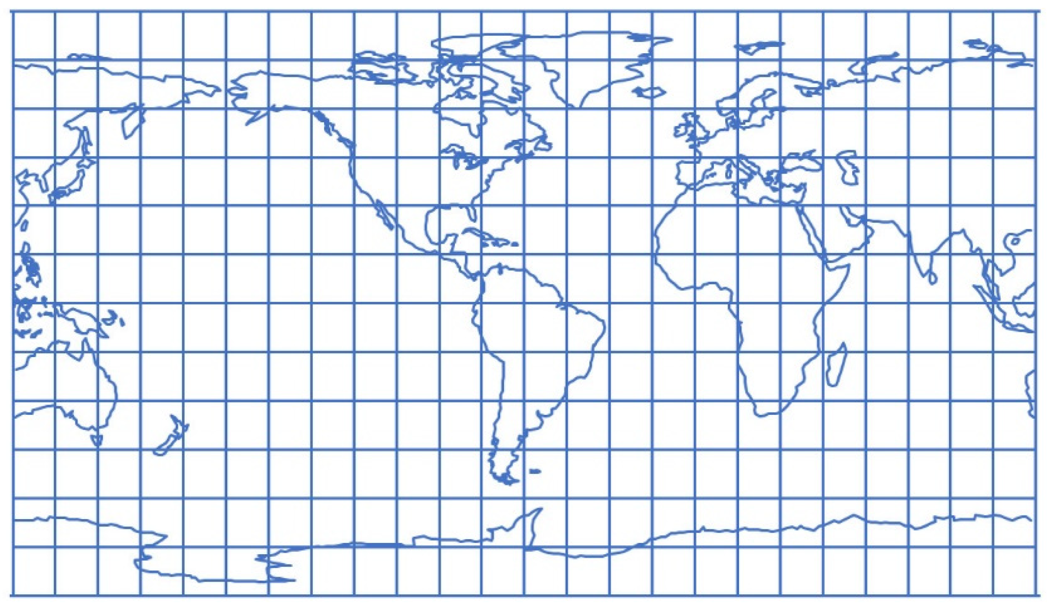
If we assume that, in a normal aspect cylindrical projection, the parallel to which the latitude corresponds is mapped equidistantly in the direction of the parallel (), the length of the image of that parallel in the projection will be equal to expression (39). Namely, the consequence of the equidistance condition will be that the equation for the abscissa x is of the form
where is the longitude of the central meridian of the mapped area. From (49), it is immediately seen that the length of each parallel in the projection plane is equal to the expression (39), including the one to which the latitude corresponds (Figure 3).
5.2. Example 2
Let us suppose that the equations of a normal aspect cylindrical projection reads
It is easy to calculate
and then, according to (11)
Considering (18), we have
If we assume that for some normal aspect cylindrical projection given by (50), the parallel corresponding to the latitude is mapped equidistantly in the direction of the parallel (), then the length of the image of that parallel in the projection plane will be equal to expression (39). For the cylindrical projections given by equations (50), the abscissa x is generally not proportional to the longitude. Let us look, for example, at the projection given by the equations (Figure 4).
We calculate
and then, considering (11)
and, by (18)
The length of each parallel in the projection given by Equations (54) will be equal to , i.e., equal to the length of the equator of the sphere of radius R. From (57), we can read that for that projection, k depends on both and , and that it will be only for the longitude λ for which holds. Therefore, in that projection, there are no equidistantly mapped parallels in the direction of the parallels.
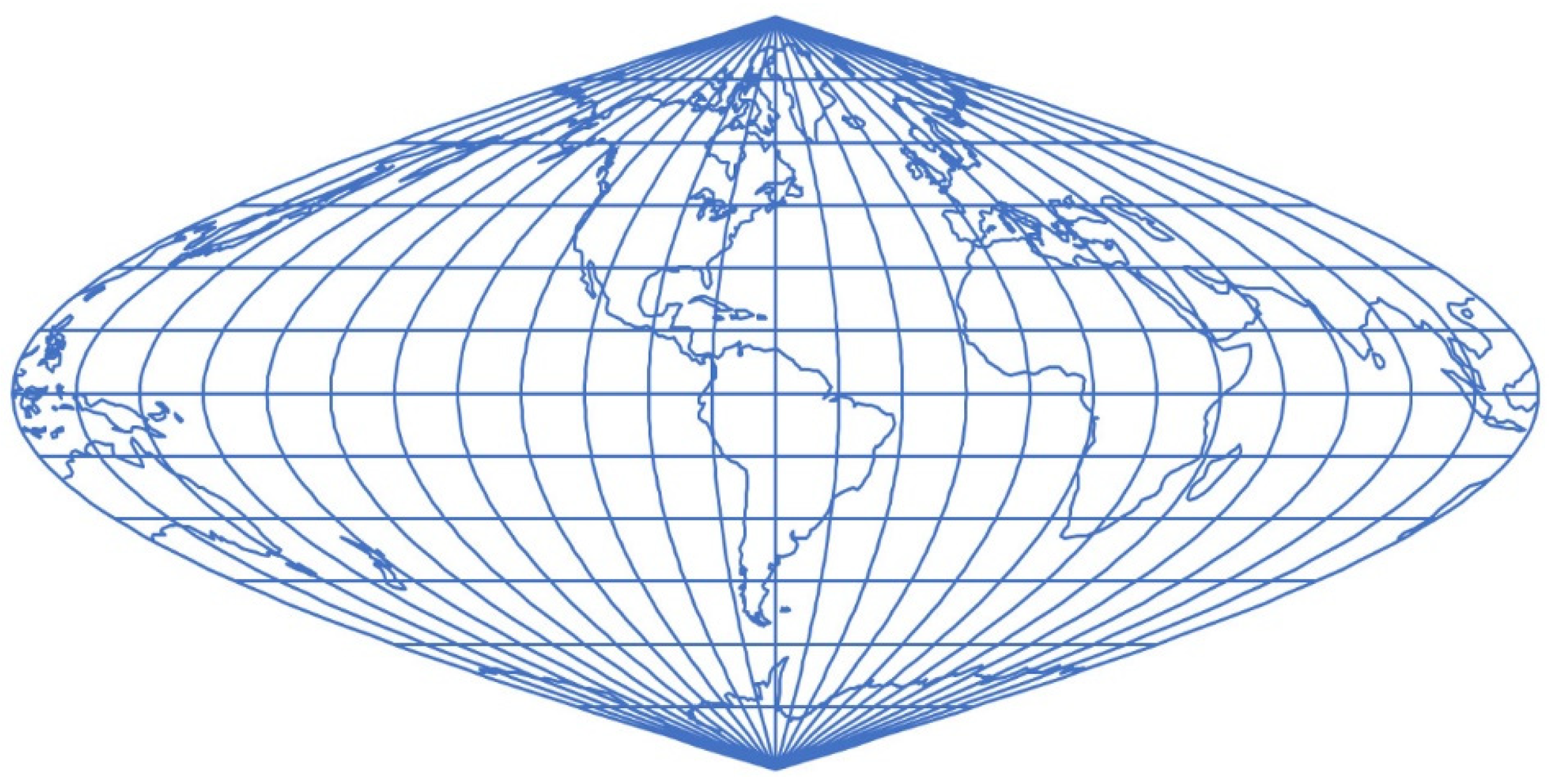
Analogous reasoning also applies to pseudocylindrical projections, where the abscissa x is proportional to the longitude . However, for some pseudocylindrical projections, the abscissa x is not proportional to the longitude (Figure 5). Let us look, for example, at the projection given by the equations
Let us calculate
then, by (11) and (59)
and then, by (18)
From (61), we can read that for that projection, k does not depend on , and that it will be only for the longitude for which is valid. So, in that projection, there is not a single equidistantly mapped parallel in the direction of the parallel. There are two meridians that are mapped equidistantly in the direction of the parallels.
The length of the parallel to which the latitude corresponds in the projection is , which is equal to the length of the corresponding parallel on the sphere. So, we have a map projection that does not have a single equidistantly mapped parallel, but the length of each individual mapped parallel is equal to the length of the corresponding parallel on the sphere (Figure 5).
The projection given by Equations (58) resembles the well-known sinusoidal (Sanson) projection (Figure 6):
Let us calculate
then, by (11) and (63)
and, by (18)
Figure 6.
World map shown in sinusoidal (Sanson) projection defined by Equations (62).

From (65), we can read that for that projection, k does not depend on and that in every point, . So, in that projection, all parallels are equidistantly mapped in the direction of the parallels. The length of the parallel to which the latitude corresponds in the projection is , which is equal to the length of the corresponding parallel on the sphere. So, we have a map projection in which all parallels are equidistantly mapped, so the length of each mapped parallel is equal to the length of the corresponding parallel on the sphere.
6. Conclusions
In the existing cartographic literature, standard parallels are not unambiguously defined. Therefore, in this article, we first define the standard points and then the standard parallels. It turns out to be useful to define equidistantly mapped points, and then equidistantly mapped parallels. In doing so, we must distinguish between equidistant mapping in the direction of the parallels and in the direction of the meridians. In addition, it was observed that equidistantly mapped parallels in the direction of parallels differ in principle from true length parallels.
The author proposes these definitions:
- A standard point is a point where linear distortions are equal to zero in all directions.
- A standard parallel is a parallel whose all points are standard;
- An equidistantly mapped point in the direction of the parallel passing through that point has the property , where is the linear scale factor in the direction of the parallel at that point;
- An equidistantly mapped parallel in the direction of that parallel is a parallel whose all points are equidistantly mapped in the direction of that parallel;
- An equidistantly mapped point in the direction of the meridian passing through that point has the property , where is the linear scale factor in the direction of the meridian at that point;
- An equidistantly mapped parallel in the direction of the meridian is a parallel whose points are all equidistantly mapped in the direction of that meridian;
- An equidistantly mapped meridian in the direction of the meridian, as well as an equidistantly mapped meridian in the direction of the parallels, can be defined analogously;
- A parallel of true length is a parallel whose length in the projection plane is equal to the length of that parallel on the sphere (ellipsoid).
Based on the introduced definitions, a standard parallel is also an equidistantly mapped parallel in any direction. The reverse is not valid. An equidistantly mapped parallel does not have to be a standard parallel.
Furthermore, it was shown that an equidistantly mapped parallel in the direction of that parallel is also a parallel of true length. The reverse is not valid. A parallel of true length does not have to be an equidistantly mapped parallel.
Finally, since every standard parallel is also an equidistantly mapped parallel, then every standard parallel will also be a parallel of true length. The reverse is not valid. A true length parallel does not have to be a standard parallel (Figure 7).
Funding
This research received no external funding.
Data Availability Statement
The data presented in this study are available in the article.
Conflicts of Interest
The author declares no conflicts of interest.
References
- Anthamatten, P. How to Make Maps, An Introduction to Theory and Practice of Cartography; Routledge: London, UK; New York, NY, USA, 2021. [Google Scholar]
- Šavrič, B.; Kennedy, M. Map Projections in ArcGIS. Available online: https://storymaps.arcgis.com/stories/ea0519db9c184d7e84387924c84b703f (accessed on 7 December 2021).
- Šavrič, B.; Jenny, B. Automating the selection of standard parallels for conic map projections. Comput. Geosci. 2016, 90, 202–212. [Google Scholar] [CrossRef]
- Deetz, C.H.; Adams, O.S. Elements of Map Projection with Applications to Map and Chart Construction, 4th ed.; U.S. Coast and Geodetic Survey Special Publication: Washington, DC, USA, 1934.
- Monmonier, M. Rhumb Lines and Map Wars; The University of Chicago Press: Chicago, IL, USA; London, UK, 2004. [Google Scholar]
- Van Sickle, J. GPS for Land Surveyors, 4th ed.; CRC Press, Taylor & Francis Group: Boca Raton, FL, USA, 2015. [Google Scholar]
- Bolstad, P. GIS Fundamentals: A First Text on Geographic Information Systems, 5th ed.; Eider Press: White Bear Lake, MN, USA, 2016. [Google Scholar]
- Bugayevskiy, L.M.; Snyder, J.P. Map Projections, A Reference Manual; Taylor & Francis: London/Bristol, UK, 1995. [Google Scholar]
- Kotlyakov, V.M.; Komarova, A.I. Elsevier’s Dictionary of Geography, in English, Russian, French, Spanish and German; Elsevier: Amsterdam, The Netherlands, 2007. [Google Scholar]
- Tobler, W.R. A Classification of Map Projecitions. Ann. Am. Assoc. Geogr. 1962, 52, 167–175. [Google Scholar] [CrossRef]
- Lapaine, M. On the definition of standard parallels in map projections. ISPRS Int. J. Geo-Inf. 2023, 12, 490. [Google Scholar] [CrossRef]
- Kavrayskiy, V.V. Izbrannye Trudy, Tom II, Matematicheskaja Kartografija, Vypusk 1; Izdanie Upravlenija nachal’nika Gidrograficheskoy Sluzhby VMF: USSR, 1958. [Google Scholar]
- Biernacki, F. Theory of Representation of Surfaces for Surveyors and Cartographers; Translated from Polish; U.S. Department of Commerce: Washington, DC, USA, 1965.
- Richardus, P.; Adler, R.K. Map Projections; North-Holland: Amsterdam, The Netherlands; London, UK, 1972. [Google Scholar]
- Maling, D.H. Coordinate Systems and Map Projections; George Philip and Son: London, UK, 1973. [Google Scholar]
- Snyder, J.P. Map Projections—A Working Manual; U.S. Geological Survey Professional Paper 1395; USGS Publications: Washington, DC, USA, 1987. [Google Scholar]
- Snyder, J.P.; Voxland, P.M. An Album of Map Projections; U.S. Geological Survey Professional Paper 1453; Reprinted 1994 with Corrections; USGS Publications: Washington, DC, USA, 1989; p. 249. [Google Scholar]
- Bugayevskiy, L.M. Matematicheskaja Kartografija; Zlatoust: Moscow, Russia, 1998. [Google Scholar]
- Kerkovits, K.A. Map Projections. Lecture Notes for students in Cartography and Geoinformatics. MSc programme, Eötvös Loránd University, Budapest, Hungary, 2022. [Google Scholar]
- Snyder, J.P. Equidistant Conic map projections. Ann. Am. Assoc. Geogr. 1978, 68, 373–383. [Google Scholar] [CrossRef]
- Canters, F. Small-Scale Map Projection Design; Taylor & Francis: London, UK; New York, NY, USA, 2002. [Google Scholar]
- Lapaine, M.; Frančula, N.; Tutek, Ž. Local linear scale factors in map projections in the direction of coordinate axes. Geo-Spat. Inf. Sci. 2021, 24, 630–637. [Google Scholar] [CrossRef]
- Hinks, A.R. Map Projections, 2nd ed.; Cambridge University Press: Cambridge, UK, 1921; p. 158. [Google Scholar]
Figure 1.
Northern hemisphere in the normal aspect orthographic projection.

Figure 2.
A hemisphere in the transverse orthographic projection.

Figure 3.
World map in an equidistant cylindrical projection for which . The length of all parallels in the projection is . This length is equal to the length of the parallel on the sphere to which latitude 30° corresponds.
Figure 3.
World map in an equidistant cylindrical projection for which . The length of all parallels in the projection is . This length is equal to the length of the parallel on the sphere to which latitude 30° corresponds.

Figure 4.
Map of the world in cylindrical projection given by Equations (54).

Figure 5.
World map shown in the projection defined by Equations (58).

Figure 7.
Every standard parallel is an equidistantly mapped parallel, and every equidistantly mapped parallel in the direction of the parallel is a true length parallel. The opposite need not be true.
Figure 7.
Every standard parallel is an equidistantly mapped parallel, and every equidistantly mapped parallel in the direction of the parallel is a true length parallel. The opposite need not be true.

Disclaimer/Publisher’s Note: The statements, opinions and data contained in all publications are solely those of the individual author(s) and contributor(s) and not of MDPI and/or the editor(s). MDPI and/or the editor(s) disclaim responsibility for any injury to people or property resulting from any ideas, methods, instructions or products referred to in the content. |
© 2024 by the author. Licensee MDPI, Basel, Switzerland. This article is an open access article distributed under the terms and conditions of the Creative Commons Attribution (CC BY) license (https://creativecommons.org/licenses/by/4.0/).
Share and Cite
MDPI and ACS Style
Lapaine, M. Parallels in Cartography: Standard, Equidistantly Mapped and True Length Parallels. Geographies 2024, 4, 52-65. https://doi.org/10.3390/geographies4010004
AMA Style
Lapaine M. Parallels in Cartography: Standard, Equidistantly Mapped and True Length Parallels. Geographies. 2024; 4(1):52-65. https://doi.org/10.3390/geographies4010004
Chicago/Turabian StyleLapaine, Miljenko. 2024. "Parallels in Cartography: Standard, Equidistantly Mapped and True Length Parallels" Geographies 4, no. 1: 52-65. https://doi.org/10.3390/geographies4010004