OpenDroneMap: Multi-Platform Performance Analysis

Abstract

This paper analyzes the performance of the open-source OpenDroneMap image processing software (ODM) across multiple platforms. We tested desktop and laptop computers as well as high-performance cloud computing and supercomputers. Multiple machine configurations (CPU cores and memory) were used. We used eBee S.O.D.A. drone image datasets from Namibia and northern Finland. For testing, we used the OpenDroneMap command line tool with default settings and the fast orthophoto option, which produced a good quality orthomosaic. We also used the “rerun-all option” to ensure that all jobs started from the same point. Our results show that ODM processing time is dependent upon the number of images, a high number of which can lead to high memory demands, with low memory leading to an excessively long processing time. Adding additional CPU cores is beneficial to ODM up to a certain limit. A 20-core machine seems optimal for a dataset of about 1000 images, although 10 cores will result only in slightly longer processing times. We did not find any indication of improvement when processing larger datasets using 40-core machines. For 1000 images, 64 GB memory seems to be sufficient, but for larger datasets of about 8000 images, higher memory of up to 256 GB is required for efficient processing. ODM can use GPU acceleration, at least in some processing stages, reducing processing time. In comparison to commercial software, ODM seems to be slower, but the created orthomosaics are of equal quality.

1. Introduction

This paper analyzed the performance of OpenDroneMap (ODM) open-source image processing software over multiple platforms. These platforms included laptops, desktops, Linux-based high-performance cloud computing, and supercomputing infrastructures. The idea of open-source software is not new and is continuously gaining interest [1,2,3,4,5]. This is more so because of the huge success of widely used open-source software like QGIS, R [6], and open-source operating systems like Linux [1,7]. In general terms, the idea of open-source software is such that its development and maintenance are performed collectively by a community of people with a shared interest [1,2,7]. Open-source software is a strategy that has been used by many industries for long-term sustainability purposes [8]. Thus, maintaining the quality of open-source software is important [9,10,11].

High Performance Computing (HPC) supercomputers have long been used in the scientific community [12,13]. For example, CSC (the Finnish national IT center for science) has had HPC machines for the past 40 years. Cloud computing, on the other hand, is a relatively new concept, which evolved over the last 10 years. Cloud computing offers instant access to computing resources at different scales based on user needs [14,15]. Cloud computing and supercomputing provide the ability to run multiple parallel computing tasks to be processed, saving time and money [14,16,17]. One of the features of cloud computing is the virtualized framework that provides users access to hardware, software, and data storage services [18]. With this virtualized framework, users can install multiple applications for different purposes [17,18,19]. The use of virtualization technologies allows users to deploy multiple virtual machines (VM) in a consolidated data center [17,20,21]. These virtualized frameworks give users administrative privileges to install and run software using the host’s resources. In other words, instead of having to buy an expensive high-performance personal computer, a user can launch a temporal, virtual machine to perform a specific project [14]. As such, software like ODM can be installed on a cloud virtual machine where the user has full and sole control (administrator) privileges. On the other hand, if ODM is installed on a supercomputer, all users will have access to it, which provides services to a wider user community. On a supercomputer, the user must wait in a batch queue for processing, which can make a cloud virtual machine more flexible.

The main goal of this study was to test the performance of ODM (version 3) across multiple platforms using the default settings.

To our knowledge, no peer-reviewed scientific publication has conducted an analysis of ODM’s performance, a free drone-mapping software. Currently, only a few software packages are available that facilitate the processing of drone images, most of which are commercial, such as MetaShape or Pix4D. Therefore, our research not only stands out as unique and timely but also makes a valuable contribution to the scientific community.

The result of this study will form the baseline for future research in this area. To achieve this, we used personal laptops, desktops, and CSC’s (the Finnish national IT center for science) different cloud computing virtual machine flavors (pre-defined core and memory combinations), and a supercomputer. Specifically, we used the cPouta cloud computing services and the Puhti supercomputer.

In addition, we tested graphical processing units (GPU) on the Puhti supercomputer system, as well as on a high-performance desktop and two laptops, all equipped with NVIDIA GPUs.

2. Materials and Methods

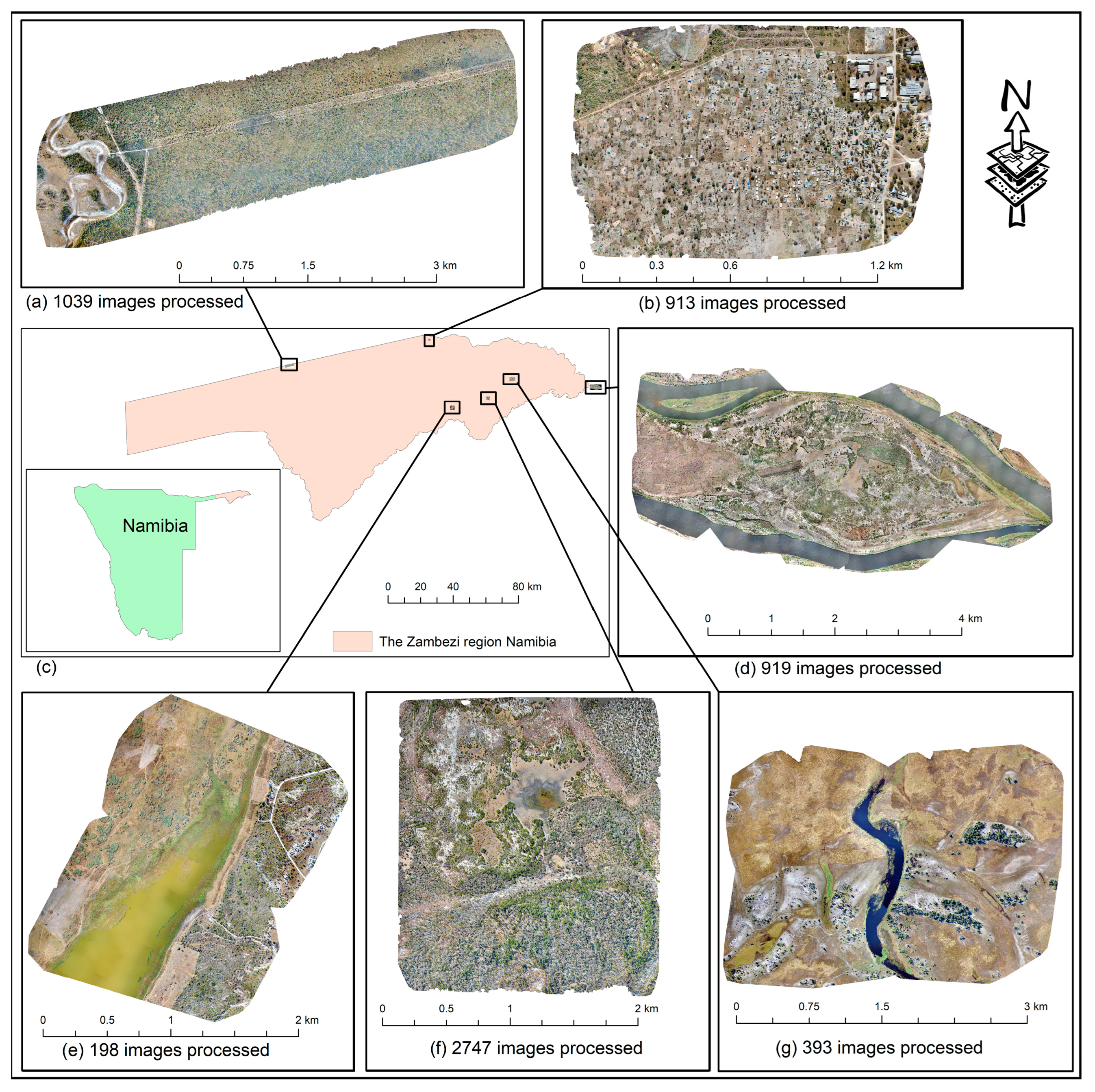
2.1. Data

We used two aerial drone image datasets with varying numbers of images and geographical settings. One set of images of subtropical forest and floodplain environments were collected in northeastern Namibia in July 2017. The drone data in Namibia were collected in six different locations that included lakes (198 images), floodplains (393 images), forests (913 images), settlements (1039 images), and conservation areas (2747 images). An additional 7917 images of a northern boreal area were collected in northern Finland in 2019. The images were collected using a SenseFly eBee Plus (senseFly.com (accessed on 21 March 2023)), fixed-wing drone. The eBee camera model was the SenseFly S.O.D.A. (Sensor Optimized for Drone Applications). The eBee image dimensions were 5471 × 3648, with both vertical and horizontal resolution of 72 dpi. The images were traditional three-band RGB (red, green, and blue) true color georeferenced Tiff digital images.

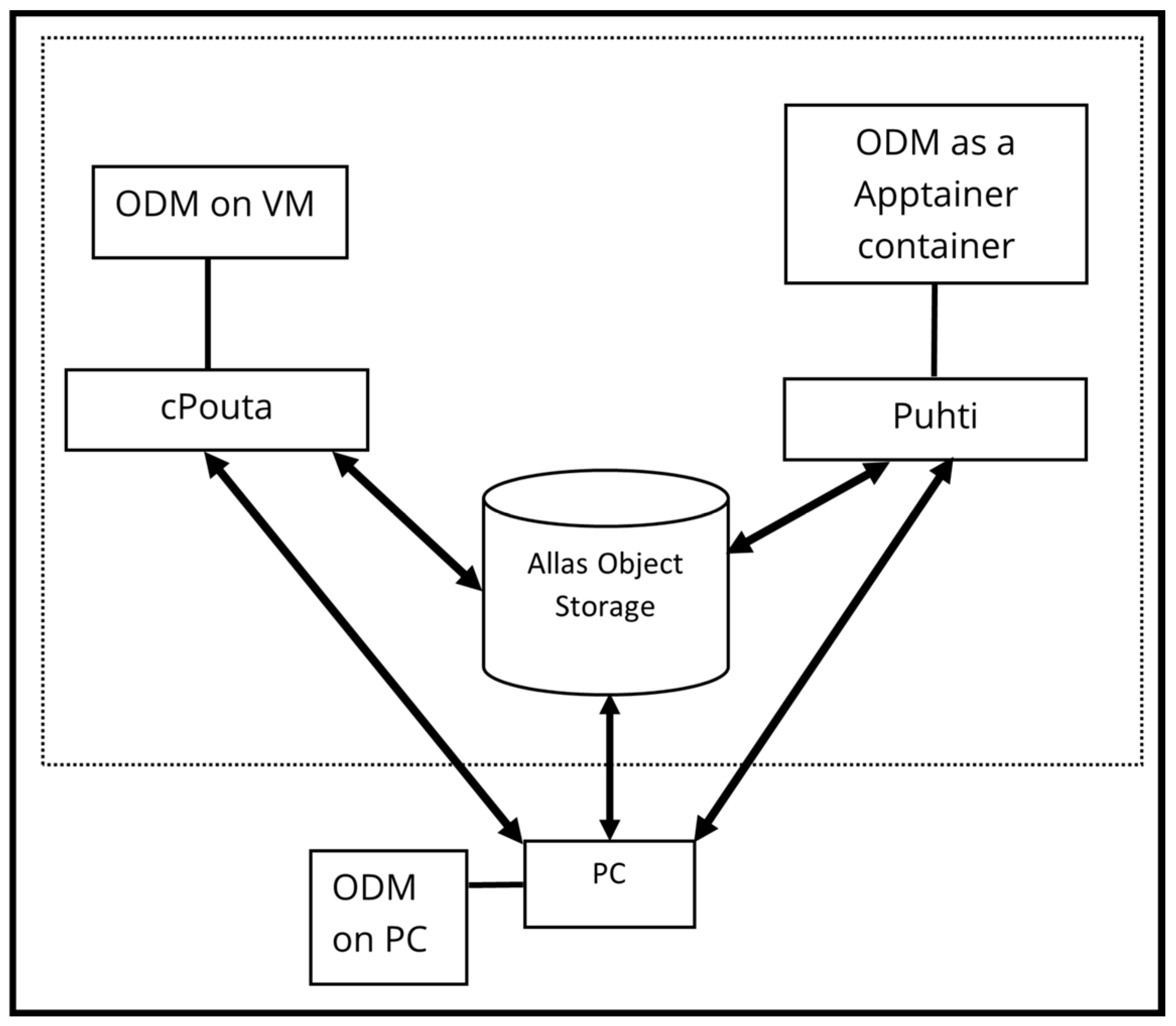
2.2. Computing Environments for ODM Performance Testing

ODM is an open-source software system for drone mapping and 3D modeling. The images are obtained by flying a pre-defined overlapping flight path over a study area using readily available free pre-flight planning software. Once the data have been acquired, they can be processed using ODM to rectify and stitch the hundreds or thousands of images into one topographically corrected orthomosaic. ODM produces 3D visualizations and digital elevation models (DEM) and offers the possibility to calculate volumes of stockpiles. In addition, ODM supports the processing of images captured using traditional digital cameras, drone RGB, and multi-spectral cameras. Furthermore, ODM can cut aerial videos into still images and subsequently produce orthoimages from them [22].

ODM is available for several configurations, and the basic version is used with a command-line interface or Linux script. A second option is WebODM, which is a server setup with a graphical user interface where the server can be a remote or local machine. For distributed computing, NodeODM and ClusterODM are also available. The simplest installation of all ODM options is performed using the cross-platform Docker-based environment (www.docker.com, accessed on 20 April 2023). As such, ODM runs on any computer that has the Docker environment installed, whether it is running Linux (any distribution that supports docker), Mac (macOS Sierra 10.12 or higher), or Windows (Windows 7 or higher). The Docker system uses part of the total available RAM memory, and sometimes swapping fills up the disk space, which can only be reclaimed by purging everything from the Docker system. The computer resources used by Docker can be adjusted and fine-tuned using the Docker settings. In our test environment, we used ODM version 3 for consistency and ease of implementation. For more information on ODM and its options, please refer to the project’s web pages (https://opendronemap.org/, (accessed on 20 April 2023)). It should be noted that, like all open-source software, ODM is constantly evolving, and new versions are released at a rapid pace, while updated documentation often lags behind.

ODM is designed in a modular fashion (Figure 1) and requires configuring numerous parameters to optimize the processing environment. ODM is optimized for parallel computing, resulting in faster execution on machines equipped with multiple CPU cores. Certain stages of ODM can utilize a graphical processing unit (GPU). The minimum requirements for running ODM include a computer with a 64bit CPU manufactured in 2010 or after, 20 GB of disk space, and 4 GB of RAM [22]. However, processing large datasets (>1000) will necessitate a minimum of 32 GB, preferably 64 GB of memory, as well as ample disk storage space.

For ODM performance testing, we used three different computing environments:

• Cloud computing virtual machines.
• A supercomputer
• A high-end Personal Computer (PC) and two laptops

For cloud computing and supercomputer, we used the computing facilities of CSC—IT center for science (www.csc.fi, accessed on 20 April 2023). Specifically, we used the cPouta cloud and Puhti supercomputer, together with the Allas object storage facility (Figure 2).

cPouta is an Infrastructure as a Service (IaaS) cloud platform [23] that is built upon OpenStack [24]. The cPouta cloud services can be accessed via the internet and used by clients for various computational needs [23]. The cPouta IaaS offers users the ability to create and run personal virtual machines (VMs) that simulate the working environment of a traditional computer [25]. The cPouta environment provides different flavors with varying computing resources and features for launching virtual machines.

On cPouta, we used two different virtual machine flavor types: hpc4 and hpc5, each with distinct characteristics (

Table 1. cPouta hpc4 and hpc5 flavors arranged in increasing number of cores.

Flavor	Number of Cores	Memory (GB)
hpc.4.5core	5	21
hpc.4.10core	10	42
hpc.5.16core	16	58
hpc.4.20core	20	85
hpc.5.32core	32	116
hpc.4.40core	40	171
hpc.5.64core	64	232

). These flavors have a fixed number of cores and memory, which users can launch as virtual machines.

The data volume and subsequent storage requirements grow exponentially with an increasing number of images, resulting in huge storage demands. To resolve this storage problem, we stored our data in the Allas object storage system (Figure 2). From our tests, running 7917 images using the default settings required about 700 GB of storage space. For this purpose, we used a separate disk volume that was mounted to the cPouta virtual machine (VM). The cPouta VMs have a default disk storage of only 80 GB, which is insufficient for most ODM jobs involving more than 100 images.

The Puhti supercomputer has 682 CPU and 80 GPU nodes. Each CPU node has 40 cores, while each GPU node has 40 CPU cores and 4 GPUs. The peak performance of the CPU partition is rated as 1.8 petaflops and the peak performance of the 80 GPU partition is rated as 2.7 petaflops [26]. In Puhti, computing resources can be reserved in many combinations using the SLURM job system. ODM scripts are run as batch jobs using the SLURM system.

On Puhti, it is possible to use one or more CPU cores with varying amounts of memory. However, since ODM can utilize only one node at a time, the tests were limited to 40 cores. During our testing on Puhti, we conducted experiments utilizing different core configurations, including 1, 3, 15, 25, 30, and 40 cores (

Table 2. Puhti configurations used in this study.

Number of Cores	Memory Per Core (GB)
1	20
3	20
5	20
15	8
20	5
25	8
30	5
40	3

). When it came to GPU testing on Puhti, we were limited to 5, 10, and 20 cores due to the high demand and long queues for GPU cores. The availability of GPU cores was not always immediate, making them less readily accessible for our experiments.

The OpenDroneMap software is installed in Puhti as a non-root Apptainer container, and in cPouta and laptop personal computers (PC) as Docker containers. Puhti uses the Lustre parallel storage, with a total space of 4.8 PB, and is configured into three sections: home (user home directory, 10 GB), projappl (installation of applications, 50 GB), and scratch (temporary space for script used in testing and running jobs, 1 TiB) [26]. During our test, we stored the data on the scratch disk.

For permanent storage of data, the Allas service provides a modern general-purpose object-storage service. It has the S3 and Swift interfaces on CEPH storage. CEPH is a highly efficient open-source distributed file system that offers the capability to store data as single files or objects in blocks [27,28,29]. Not only does CEPH provide superior performance, scalability, and reliability, but it also ensures efficient data management [27,28,29]. On Allas, data is stored as objects in buckets, where the objects can either be a file, image, or packed (zipped) folder [30].

In addition, we ran tests on three different local Windows computers; a Windows 10 desktop and two Windows 11 laptops. These were High-End I7 and I9 multi-core machines with 64 GB RAM. A technical summary of all used computing environments is given in

Table 3. Characteristics of used computing environments.

Flavor	CPU	GPU	CPU Cores	Memory, GB
cPouta hpc4	Intel(R) Xeon(R) Gold 6148 CPU @ 2.40 GHz, hyper-threading	-	5–40	21–171
cPouta hpc5	AMD EPYC 7702 64-Core Processor, boost up to 3.35 GHz	-	16–64	58–232
Puhti supercomputer	Intel Xeon Gold 6230 2.1 GHz	NVIDIA Volta V100	1–40	1–240 (up to 1500 available)
64-bit laptop W11	11th Gen Intel(R) Core (TM) i7-11800H @ 2.30 GHz 2.30 GHz	NVIDIA T1200	8	64
64-bit laptop W11	11th Gen Intel(R) Core (TM) i9-11950H @ 2.60 GHz 2.61 GHz	NVIDIA T1200	8	64
64-bit desktop W10	Intel(R) Core (TM) i9-7980XE CPU @ 2.60 GHz 2.59 GHz	NVIDIA Quadro P4000	18	64

.

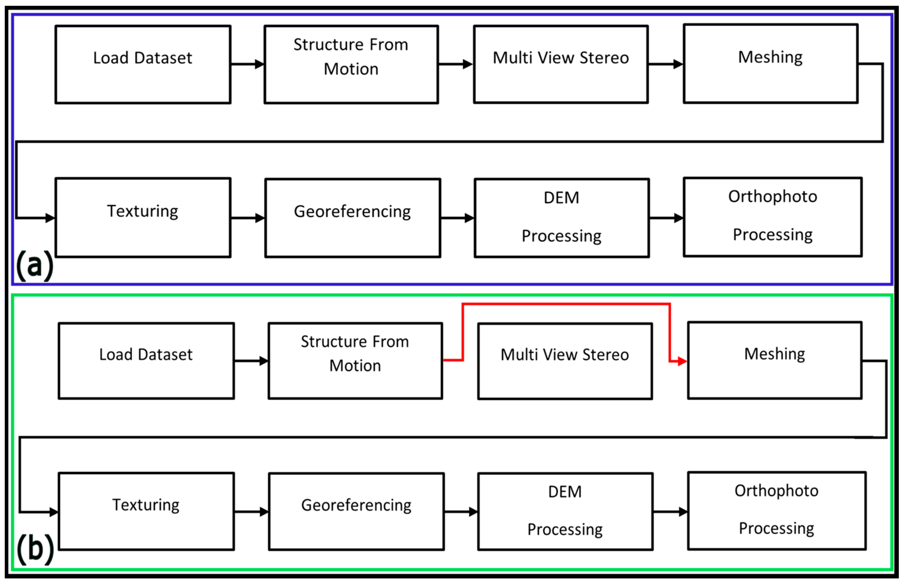
2.3. Testing Configuration

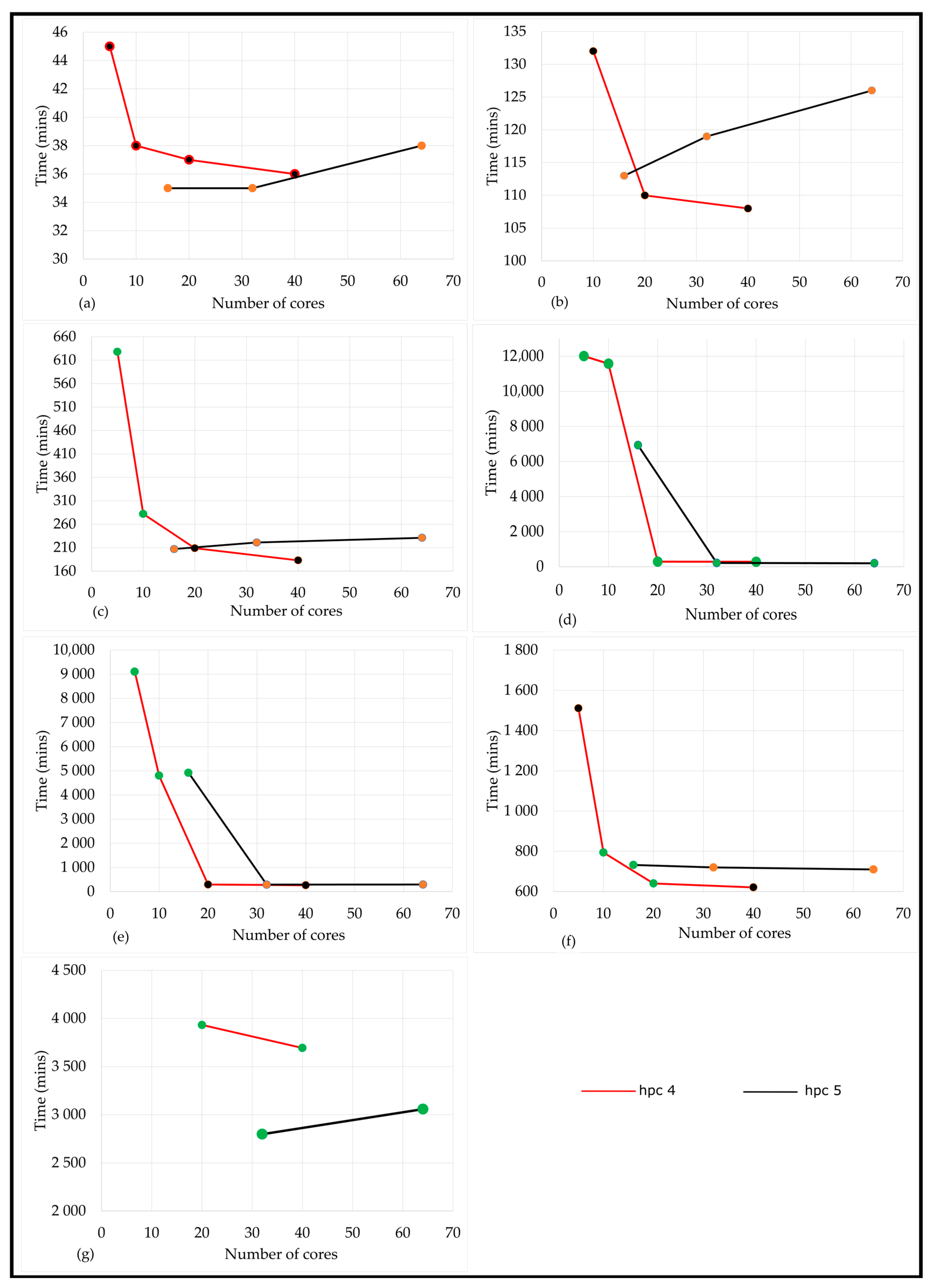
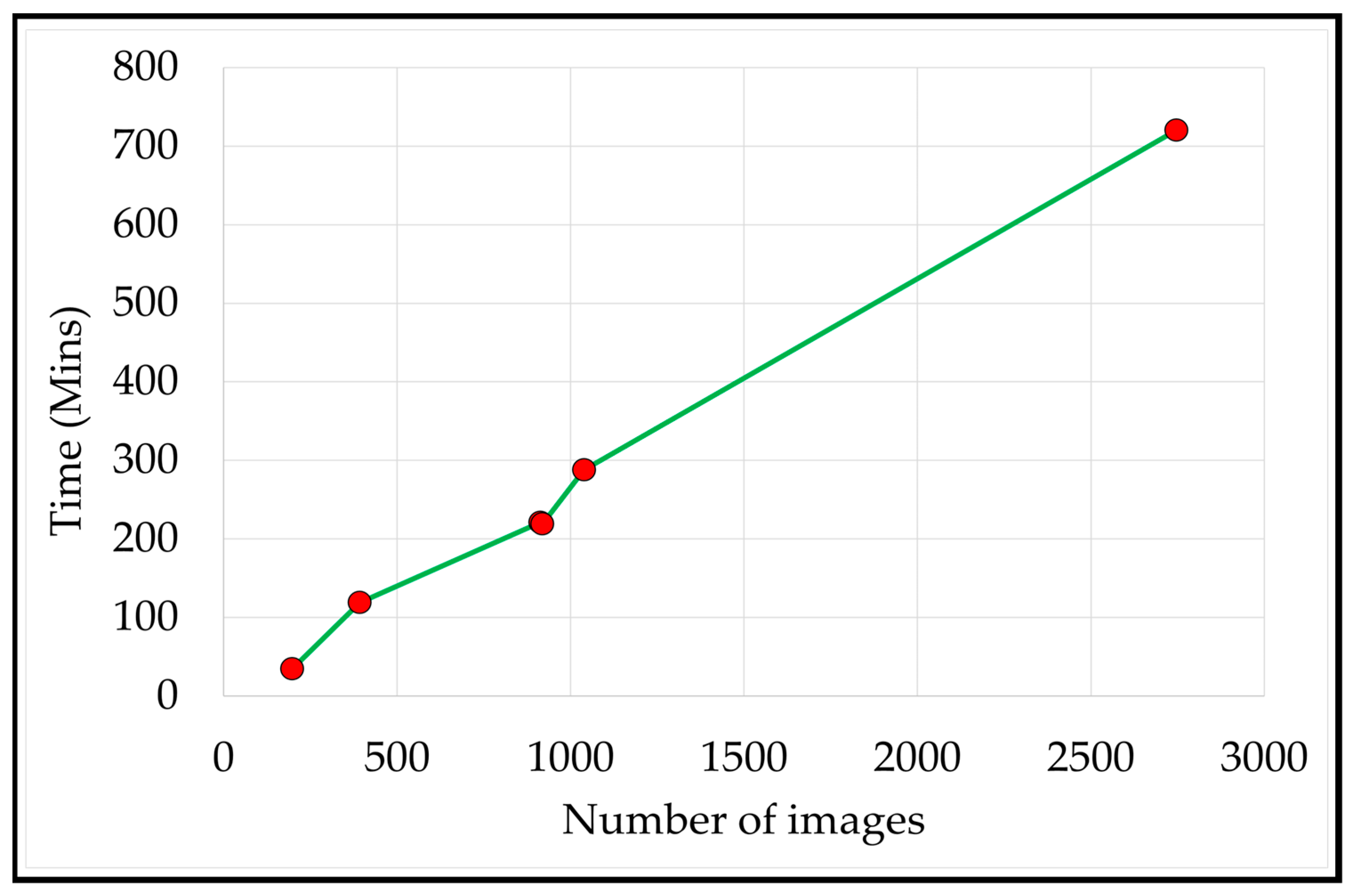
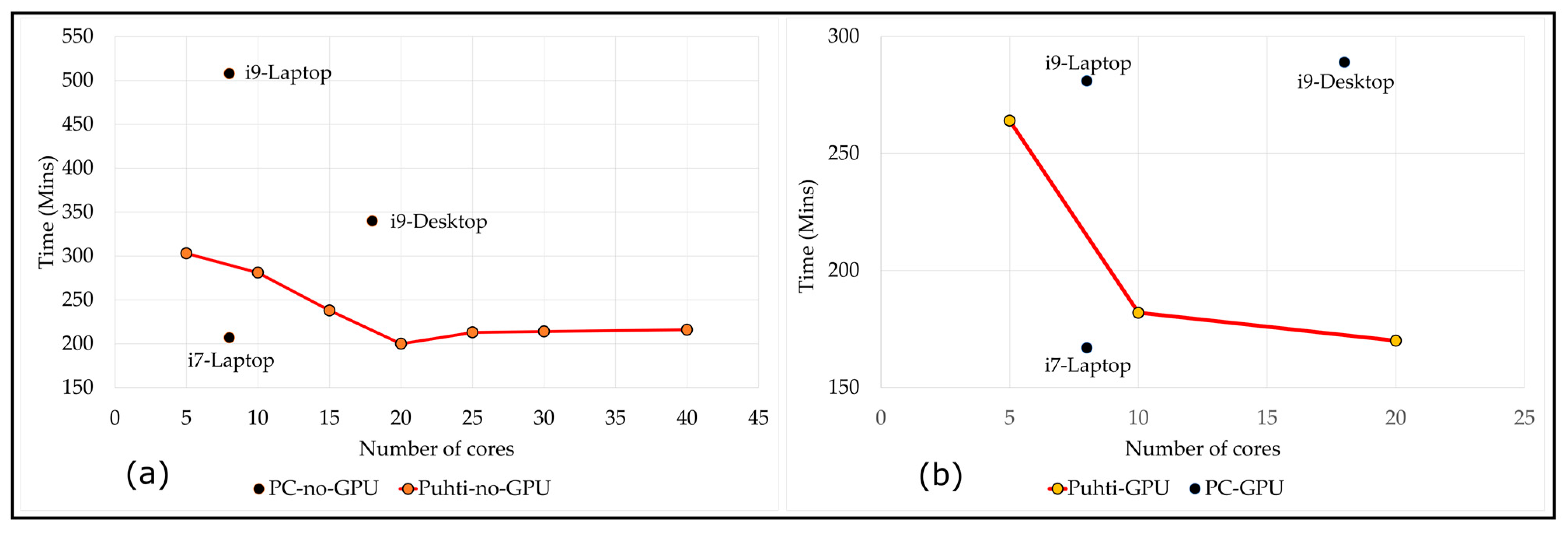
We used the 1039 images (subtropical forest) test runs as a benchmark across all the platforms: local laptops, desktop, cPouta cloud, and Puhti supercomputer. Additionally, we ran different groups of image datasets (198, 393, 913, 919, 1039, and 2747 images) on several cPouta VMs.

To create the virtual machines (VMs) on the cloud platform, we utilized the hpc4 and hpc5 flavors. Each flavor offered different configurations of cores and available memory, as shown in Table 1. This allowed us to tailor the VM specifications according to our needs and optimize performance.During the execution of the ODM software, we used the default settings and the ‘fast orthophoto’ option (Figure 1b) since we only required the orthomosaic outputs. The orthomosaic images achieved excellent quality, requiring no further adjustments to the default settings. The ‘fast orthophoto’ option bypasses the Multi-View Stereo step (Figure 1b), reducing processing time by focusing solely on the orthomosaic, which suffices for mostly flat areas.

To ensure consistent starting points for all jobs (image loading), we employed the ‘rerun-all’ option, which removes all previously generated results. In certain tests with limited memory, we employed the ‘split–merge’ option to break down the process into smaller subareas. While the split–merge option restricts memory usage, it increases processing time.

Finally, we compiled separately and plotted the results of the hpc4 and hpc5 VM flavors.

3. Results

The outcome of the cPouta tests is shown in

Table 4. Results of the cPouta virtual machine flavors. The number of images processed for each flavor and the time taken are also shown. For the 7917 images, only four VMs were tested with RAM 85 GB to 232 GB. The numbers in “brackets” indicate the number of images that we used as a parameter setting with the ODM split–merge feature because of insufficient RAM of the VMs. The split–merge indicated here corresponds to the green points in Figure 2 below.

Number of Images Processed for Each Time Column
VM Flavor	Cores	RAM	Time (hours and minutes)
			198	393	913	919	1039	2747	7917
hpc4	5	21	0:45	72:18 (100)	10:28 (100)	200:07 (100)	151:44 (100)	25:11 (100)	—
hpc4	10	42	0:38	2:12	4:42 (200)	192:53 (200)	80:02 (200)	13:14 (600)	—
hpc5	16	58	0:35	1:53	3:27	115:31 (400)	82:02 (400)	12:12 (700)	—
hpc4	20	85	0:37	1:50	3:29	4:51	4:52	10:40 (1000)	65:32 (1500)
hpc5	32	116	0:35	1:59	3:41	3:39	4:48	12:00	46:37 (500)
hpc4	40	171	0:36	1:48	3:03	4:46	4:23	10:21	61:33 (500)
hpc5	64	232	0:38	2:06	3:51	3:18	4:50	11:50	50:57 (500)

and Figure 3a–g and Figure 4, while those of the Windows desktop, laptops, and Puhti supercomputer are shown in

Table 5. Results of ODM Tests on Windows Desktops, Laptops, and Puhti Supercomputer (Full Specifications in Table 1).

System Type	Cores	Memory (GB)	Time (Hours and Minutes)		Speed Gain with GPU, %
			No GPU	With GPU
64-bit, i7 (Laptop)	8	64	3:27	2:47	19
64-bit, i9 (Laptop)	8	64	8:28	4:41	45
64-bit, i9 (Desktop)	18	64	5:40	4:49	15
Puhti supercomputer	1	60	11:48	-	-
Puhti supercomputer	3	30	6:17	-	-
Puhti supercomputer	5	100	5:03	4:24	13
Puhti supercomputer	10	100	4:41	3:02	35
Puhti supercomputer	15	120	3:58	-	-
Puhti supercomputer	20	100	3:20	2:50	15
Puhti supercomputer	25	200	3:33	-	-
Puhti supercomputer	30	240	3:34	-	-
Puhti supercomputer	40	120	3:36	-	-

and Figure 5. The ODM-processed images are shown in Figure 6. We see in Figure 4 that as the number of images increases, the processing time and the amount of memory (RAM) increase linearly, as expected. There is not much difference in time duration when processing a small number of images (Table 4, Figure 3a). For example, when processing the 198 images, the time ranges from 35 to 45 min and a small difference in processing time with the increasing number of cores. The 5-core 21 RAM VM took 45 min to process 198 images while the 64-core 232 RAM VM took 38 min (7 min difference). On the other hand, as the number of images increased to 393 (almost double in this case), the processing time tripled. The time taken to process the 393 images ranged from 1 h and 48 min to 2 h and 12 min, excluding the 72 h and 18 min where we used the split–merge option (Table 4, Figure 3b). This trend is similar for all the processed images, including the 7917 (Table 4, Figure 3f,g).

Also, the split–merge option has a noticeable effect on the fluctuating increase in processing time, particularly for limited. For instance, on a 21 GB RAM machine, it took 45 min to process 198 images, but it took 72 h and 18 min for 393 images. The processing time dropped to 10 h and 28 min but increased to 200 h and 7 min (Table 4, Figure 3b). Similarly, the 42 GB RAM VM showed a similar trend to the 21 GB VM (Table 4, Figure 3). However, the effect of the split–merge option was minimal for the VMs with higher RAM (>85 GB).

In addition, the results indicate slight differences in the performance of different VM flavors for both hpc4 and hpc5. In some cases, processing times were shorter using a VM with fewer cores compared to those with more cores (Table 4). For example, when processing the 913 images, the hpc4 40-core VM took 3 h and 3 min, while the hpc5 64-core VM took 3 h and 51 min. We believe this behavior could be attributed to the differences in hardware and swap memory processes of the VMs. Furthermore, when processing failed due to insufficient RAM, we tested the split–merge feature. The columns with numbers enclosed in brackets are the test runs where we applied the split–merge option. The number enclosed in brackets indicates the number of images used for each submodel process.

Figure 3a–g indicates the order in which the images were processed, from the lowest (198) to the highest (7917). Both hpc4 and hpc5 flavors show a similar trend: low-RAM VMs take longer times to complete processing, while high-RAM VMs are faster.

The benchmark result for 1039 images across various platforms are shown in Table 5 and Figure 5. Without using GPU, the i7 laptop (8-cores 64 GB RAM) took 3 h and 27 min to process the images, while the i9 laptop (8-cores 64 GB RAM) and i9 desktop (18-cores 64 GB RAM) took 8 h and 28 min and 5 h and 40 min, respectively. With the GPU option, the i7 laptop showed better performance, processing the images in 2 h and 47 min, compared to 4 h and 41 min for the i9 laptop and 4 h and 49 min for the i9 desktop. The speed gains were 19%, 45%, and 15% for the i7 laptop, i9 laptop, and i9 desktop, respectively.

On the other hand, processing the 1039 images on Puhti showed varying processing times, ranging from 3 h and 20 min to 11 h and 48 min. The longest time processing time was observed with the one-core 60 GB RAM setup, taking 11 h and 48 min, while the shortest time was with the 20-cores 100 GB RAM setup, taking 3 h and 20 min. The 25-core 200 GB RAM setup took 3 h and 33 min, the 30-cores 240 GB RAM setup took 3 h and 34 min, and the 40-cores 120 GB RAM setup took 3 h and 36 min to process the same set of images. The 20-core 100 GB RAM setup with GPU showed a speed gain of 15%.

Additionally, we performed a comparison by testing the same 1039-image dataset on an 18-core I9 Desktop computer using MetaShape Agisoft version 2.0.0.15597 (https://www.agisoft.com/, accessed on 20 April 2023), which is a commercial-grade software package. The processing time for the images using MetaShape was 1 h and 43 min (including aligning, meshing, and ortho-mosaic steps), faster than the 4 h and 49 min with ODM software on the PC and 2 h and 47 min on the newer i7 laptop (Table 5). It is noteworthy that the GPU chip type significantly affects the processing time. However, the orthoimage produced by ODM is of equal quality compared to that produced by MetaShape.

4. Discussion

The results indicate that adding excessive cores only marginally decreases the processing time for ODM. However, the processing time difference is more significant when using a smaller number of cores. The optimum number of cores depends on the number of images, typically around 20 cores for a 1000-image dataset. Even with a larger dataset (7917 images), there was little improvement beyond 20 cores.

The results also demonstrate that the processing time can be reduced by using the GPU-accelerated version of ODM. Depending on the computing environment (as shown in Table 5), the processing times were 15–45% faster with GPU. The total time of processing with different GPUs ranged from 2 h and 50 min to 4 h and 49 min for the 1039-image dataset. The variations can be attributed to the different GPUs used (as shown in Table 1). These findings align with Shiva’s study [31], which reported that using a GPU can greatly benefit certain stages of ODM processes, resulting 3 to 10 times faster processing, depending on the type of GPU graphics card used. Shiva’s study tested 4- and 8-core machines using both CPU and GPU. Similarly, the study by Chang et al, 2021 [14], found that GPU performance is closely related to the type of graphic card, and they also noted that in a cloud-computing environment, proper virtual machine setup can improve performance and gains.

Optimal processing times for ODM are highly dependent on memory [22], and this study confirms that finding. Larger input datasets require more memory. With large datasets, using fewer cores (1 to 5) results in longer processing times, significantly increasing the overall processing time (as shown in Table 4). Additionally, as the number of images increases, the processing time also increases (as shown in Figure 4). We also tested the split–merge functionality of ODM, which allows for the of less memory by dividing images into smaller chunks and combining the outputs of submodels in the final phase. However, using this split-merge option comes at the expense of significantly longer processing time.

Comparing our results on cPouta with the official recommendations on the ODM website shows a generally good agreement [32]. For instance, while ODM officially recommends 128 GB memory for processing 2500 images, we were able to process 2747 images with 116 GB using 32 cores (as shown in Table 4 and Figure 3f). Similarly, we processed 4000 images with 171 GB memory and a 40-core VM (result not included here), compared to the recommended 192 GB memory by ODM [32], for processing 3500 images. For datasets up to a few thousand images, 64 GB of memory appears to be sufficient, but larger datasets up to 8000 images require 256 GB memory to process.

There seems to be little or no difference in processing time between the script-based ODM and WebODM. This is expected since WebODM only adds a web browser graphical user interface, while using the same processing engine. In general, our findings align with Shiva’s report [31], which stated that doubling the number of cores can bring potential benefits but also increases the required amount of memory, leading to some positive impacts.

However, when utilizing WebODM, the graphical user interface of ODM, we achieved remarkable results by processing up to 3000 images on a Windows 11 laptop with an 8-core I9 processor and 64 GB of memory. Notably, these findings deviate from the official recommendations for processing 2500 to 3500 images on a PC laptop. This difference could potentially be attributed to advancements in technology.

5. Conclusions

Based on our observations, we have concluded that the ODM software produces good quality orthomosaics. Both the script-based ODM and the web-browser-based WebODM graphical user interface are easy to use. ODM can be run on a personal computer or laptop for datasets up to several thousands of images.

To ensure fast processing, having sufficient memory is crucial. The split–merge option of ODM allows running larger datasets with limited memory. However, this option noticeably slows down processing time. ODM also offers a split–merge feature with parallel processing using ClusterODM and NodeODM, although it was not tested in this study. Additionally, having sufficient hard drive space is important for larger datasets

Adding a GPU processor to the system configuration clearly benefit ODM, as shown in Table 5, where the processing time improvement ranged from 15% to 45%, depending on the GPU chip. In supercomputing and cloud-computing environments where GPUs are significantly more expensive, this difference is still too small to give economic benefits, but with laptops and PCs, the GPU option proved to be extremely useful.

According to our tests, ODM benefits from increasing the number of cores. For CPU efficiency, 1 to 5 cores would be optimal; however, for processing time, using 10 to 20 cores would be optimal, as adding more than 20 cores does not increase processing speed. Adding excessive cores slows down processing time due to increased overhead. Conversely, using too few cores (1 to 5) increases processing time due to limited computing resources.

The main limitation of this study was the inability to thoroughly explore various ODM settings that could impact the software performance. For instance, it is well known that increasing the quality of the generated output will increase processing time. Also, there is a need to perform robust monitoring of the hardware, cores, and available memory and how these are affecting the overall performance of the software. Additionally, the slow reading and writing speeds of cPouta and Puhti are some of the limiting factors that need to be addressed. Another aspect that needs to be considered is how the programming language used to write ODM could contribute to the performance of the software. Other issues, such as virtualization and containerization, as shown by Shah et al. 2021 [15], could also be a limiting factor in this study.

References

1. Fuggetta, A. Open Source Software—An Evaluation. J. Syst. Softw. 2003, 66, 77–90. [Google Scholar] [CrossRef]
2. Wang, J.; Shih, P.C.; Carroll, J.M. Revisiting Linus’s Law: Benefits and Challenges of Open Source Software Peer Review. Int. J. Hum. Comput. Stud. 2015, 77, 52–65. [Google Scholar] [CrossRef]
3. Von Krogh, G.; Von Hippel, E. Special Issue on Open Source Software Development. Res. Policy 2003, 32, 1149–1157. [Google Scholar] [CrossRef]
4. Fortunato, L.; Galassi, M. The Case for Free and Open Source Software in Research and Scholarship. Philos. Trans. R. Soc. A Math. Phys. Eng. Sci. 2021, 379, 20200079. [Google Scholar] [CrossRef] [PubMed]
5. Peng, G.; Wan, Y.; Woodlock, P. Network Ties and the Success of Open Source Software Development. J. Strateg. Inf. Syst. 2013, 22, 269–281. [Google Scholar] [CrossRef]
6. R Core Team. R: A Language and Environment for Statistical Computing; R Foundation for Statistical Computing: Vienna, Austria, 2020; Available online: http://www.R-project.org/ (accessed on 20 April 2023).
7. Kogut, B.; Metiu, A. Open-Source Software Development and Distributed Innovation. Oxf. Rev. Econ. Policy 2001, 17, 248–264. [Google Scholar] [CrossRef]
8. Gamalielsson, J.; Lundell, B. Sustainability of Open Source Software Communities beyond a Fork: How and Why Has the LibreOffice Project Evolved? J. Syst. Softw. 2014, 89, 128–145. [Google Scholar] [CrossRef] [Green Version]
9. Mark, A. Achieving Quality in Open Source Software. IEEE Softw. 2007, 24, 58–64. [Google Scholar] [CrossRef]
10. Schaarschmidt, M.; Walsh, G.; von Kortzfleisch, H.F.O. How Do Firms Influence Open Source Software Communities? A Framework and Empirical Analysis of Different Governance Modes. Inf. Organ. 2015, 25, 99–114. [Google Scholar] [CrossRef]
11. Stamelos, I.; Angelis, L.; Oikonomou, A.; Bleris, G.L. Code Quality Analysis in Open Source Software Development. Inf. Syst. J. 2002, 12, 43–60. [Google Scholar] [CrossRef]
12. Geist, A.; Reed, D.A. A Survey of High-Performance Computing Scaling Challenges. Int. J. High Perform. Comput. Appl. 2017, 31, 104–113. [Google Scholar] [CrossRef]
13. Hill, Z.; Humphrey, M. A Quantitative Analysis of High Performance Computing with Amazon’s EC2 Infrastructure: The Death of the Local Cluster? In Proceedings of the IEEE/ACM International Workshop on Grid Computing, Banff, AB, Canada, 13–15 October 2009; pp. 26–33. [Google Scholar] [CrossRef]
14. Chang, A.; Jung, J.; Landivar, J.; Landivar, J.; Barker, B.; Ghosh, R. Performance Evaluation of Parallel Structure from Motion (SFM) Processing with Public Cloud Computing and an on-Premise Cluster System for Uas Images in Agriculture. ISPRS Int. J. Geoinf. 2021, 10, 677. [Google Scholar] [CrossRef]
15. Shah, S.A.R.; Waqas, A.; Kim, M.H.; Kim, T.H.; Yoon, H.; Noh, S.Y. Benchmarking and Performance Evaluations on Various Configurations of Virtual Machine and Containers for Cloud-Based Scientific Workloads. Appl. Sci. 2021, 11, 993. [Google Scholar] [CrossRef]
16. Ben Belgacem, M.; Chopard, B. A Hybrid HPC/Cloud Distributed Infrastructure: Coupling EC2 Cloud Resources with HPC Clusters to Run Large Tightly Coupled Multiscale Applications. Future Gener. Comput. Syst. 2015, 42, 11–21. [Google Scholar] [CrossRef]
17. Younge, A.J.; Henschel, R.; Brown, J.T.; von Laszewski, G.; Qiu, J.; Fox, G.C. Analysis of Virtualization Technologies for High Performance Computing Environments. In Proceedings of the 2011 IEEE 4th International Conference on Cloud Computing, Washington, DC, USA, 4–9 July 2011; pp. 9–16. [Google Scholar] [CrossRef] [Green Version]
18. Wang, L.; von Laszewski, G.; Younge, A.; He, X.; Kunze, M.; Tao, J.; Fu, C. Cloud Computing: A Perspective Study. New Gener. Comp. 2010, 28, 137–146. [Google Scholar] [CrossRef] [Green Version]
19. Huang, W.; Liu, J.; Abali, B.; Panda, D.K. A Case for High Performance Computing with Virtual Machines. In Proceedings of the 20th Annual International Conference on Supercomputing, Cairns, Australia, 28 June–1 July 2006. [Google Scholar] [CrossRef]
20. Dillon, T.; Wu, C.; Chang, E. Cloud Computing: Issues and Challenges. In Proceedings of the International Conference on Advanced Information Networking and Applications, Perth, Australia, 20–23 April 2010; pp. 27–33. [Google Scholar] [CrossRef]
21. Mauch, V.; Kunze, M.; Hillenbrand, M. High Performance Cloud Computing. Future Gener. Comput. Syst. 2013, 29, 1408–1416. [Google Scholar] [CrossRef]
22. Toffanin, P. OpenDroneMap: The Missing Guide a Practical Guide to Drone Mapping Using Free and Open Source Software; Independently Publisher: Traverse City, MI, USA, 2019. [Google Scholar]
23. CSC. What Is Pouta—Docs CSC. Available online: https://docs.csc.fi/cloud/pouta/pouta-what-is/ (accessed on 17 March 2023).
24. An Open Infra Project Open Source Cloud Computing Platform Software—OpenStack. Available online: https://www.openstack.org/software/ (accessed on 17 March 2023).
25. CSC-Cloud Cloud—Docs CSC. Available online: https://docs.csc.fi/cloud/ (accessed on 17 March 2023).
26. CSC. Puhti—Docs CSC. Available online: https://docs.csc.fi/computing/systems-puhti/ (accessed on 10 March 2023).
27. Meyer, S.; Morrison, J.P. Supporting Heterogeneous Pools in a Single Ceph Storage Cluster. In Proceedings of the 17th International Symposium on Symbolic and Numeric Algorithms for Scientific Computing (SYNASC), Timisoara, Romania, 21–24 September 2015; pp. 352–359. [Google Scholar] [CrossRef]
28. Tang, X.; Yao, X.; Liu, D.; Zhao, L.; Li, L.; Zhu, D.; Li, G. A Ceph-Based Storage Strategy for Big Gridded Remote Sensing Data. Big Earth Data 2022, 6, 323–339. [Google Scholar] [CrossRef]
29. Zhang, X.; Gaddam, S.; Chronopoulos, A.T. Ceph Distributed File System Benchmarks on an OpenStack Cloud. In Proceedings of the 2015 IEEE International Conference on Cloud Computing in Emerging Markets (CCEM), Bangalore, India, 25–27 November 2015; pp. 113–120. [Google Scholar] [CrossRef]
30. CSC. Introduction to Allas Storage Service—Docs CSC. Available online: https://docs.csc.fi/data/Allas/introduction/ (accessed on 29 March 2023).
31. Shiva Hardware Recommendations—CPU Cores, Graphics Card, CUDA, NVIDIA, Memory, RAM, Storage—Learning Area—OpenDroneMap Community. Available online: https://community.opendronemap.org/t/hardware-recommendations-cpu-cores-graphics-card-cuda-nvidia-memory-ram-storage/13705 (accessed on 6 April 2023).
32. Installation and Getting Started—OpenDroneMap 3.0.5 Documentation. Available online: https://docs.opendronemap.org/installation/#quickstart (accessed on 17 March 2023).
Figure 1. OpenDroneMap (ODM) processing pipeline: Normal processing pipeline (a) and Fast Orthophoto processing pipeline (b) (Modified with permission from [22]. Copyright 2019, Piero Toffanin).
Geographies 03 00023 g001
Figure 2. Structural arrangement of the CSC cloud and supercomputing system.
Geographies 03 00023 g002
Figure 3. The output of ODM tested on cPouta hpc4 and hpc5 Virtual Machine (VM) flavors: 198 images (a), 393 images (b), 913 images (c), 919 images (d), 1039 images (e), 2747 images (f), and 7917 images (g). We did not plot the 72 h 18 min time point for the 5-core VM flavor (see Table 4) to make this graph more legible. The points in green (cg) represent the data that we processed using the ODM split–merge option (see also Table 4 above). The hpc4 flavor is shown in red line, while the hpc5 is in black.
Geographies 03 00023 g003
Figure 4. The increase in processing time with number of images in cPouta.
Geographies 03 00023 g004
Figure 5. Comparison of ODM results for 1039 Drone Images Processed on PC and Puhti: No GPU (a) and with GPU (b). The PC results are represented as black dots, while the Puhti results are depicted as red lines.
Geographies 03 00023 g005
Figure 6. The output of ODM-processed drone images from in Namibia used in the benchmark test across various platforms. Forest reserve (a), settlement (b), locations of data collection (c), Island (d), lake (e), conservation area (f), and floodplain (g).
Geographies 03 00023 g006