
Conflicts of Interest and Emissions from Land Conversions: State of New Jersey as a Case Study

 , , ,
, , ,  , ,
, ,
Abstract
:1. Introduction
The Role of Soils in New Jersey Global Warming Response Act
2. Materials and Methods
3. Soil Carbon Regulating Ecosystem Services and Land Cover Change in the State of New Jersey
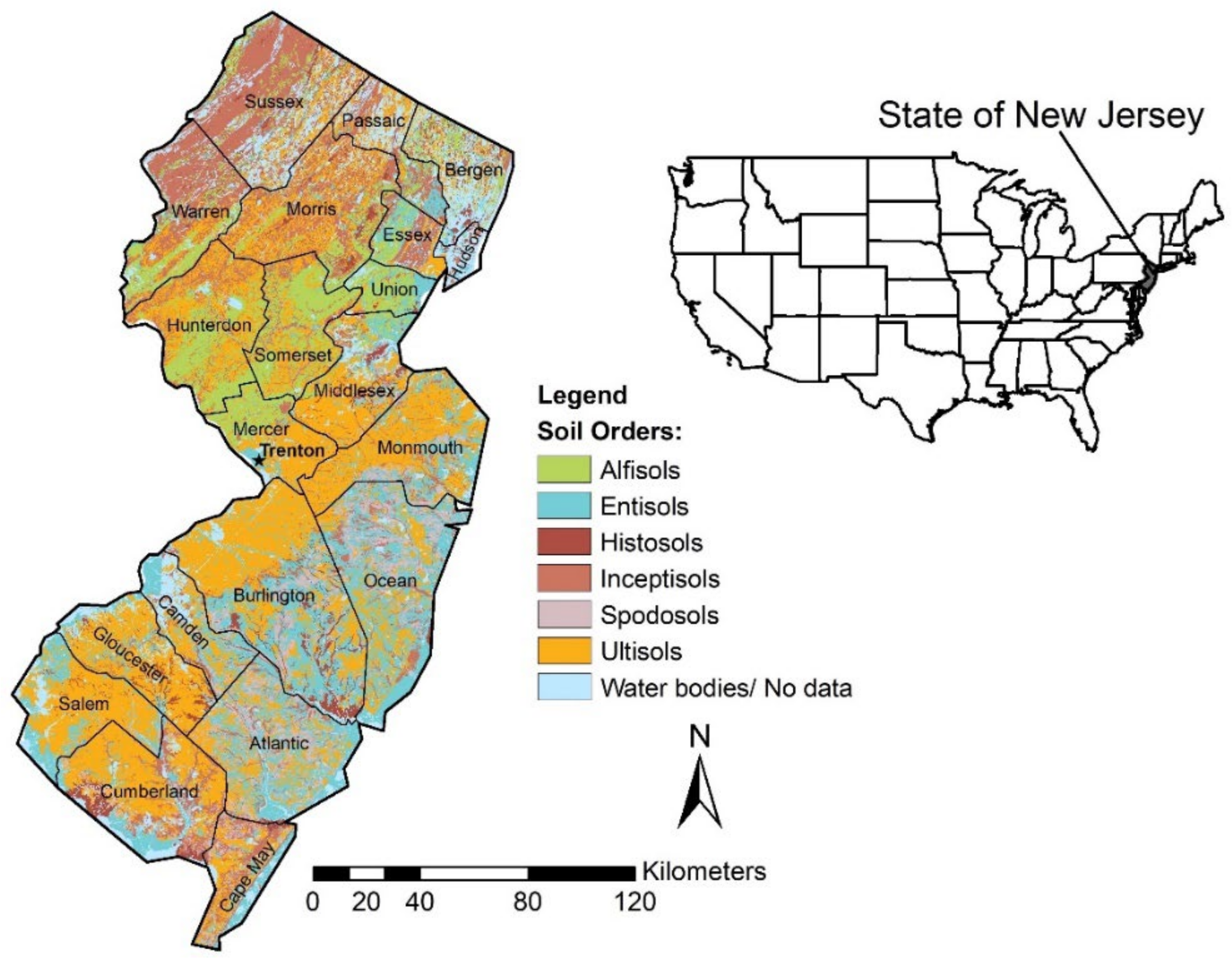
3.1. Value of SOC by Soil Order and County for New Jersey
3.2. Value of SIC by Soil Order and County for New Jersey
3.3. Value of TSC (SOC + SIC) by Soil Order and County for New Jersey
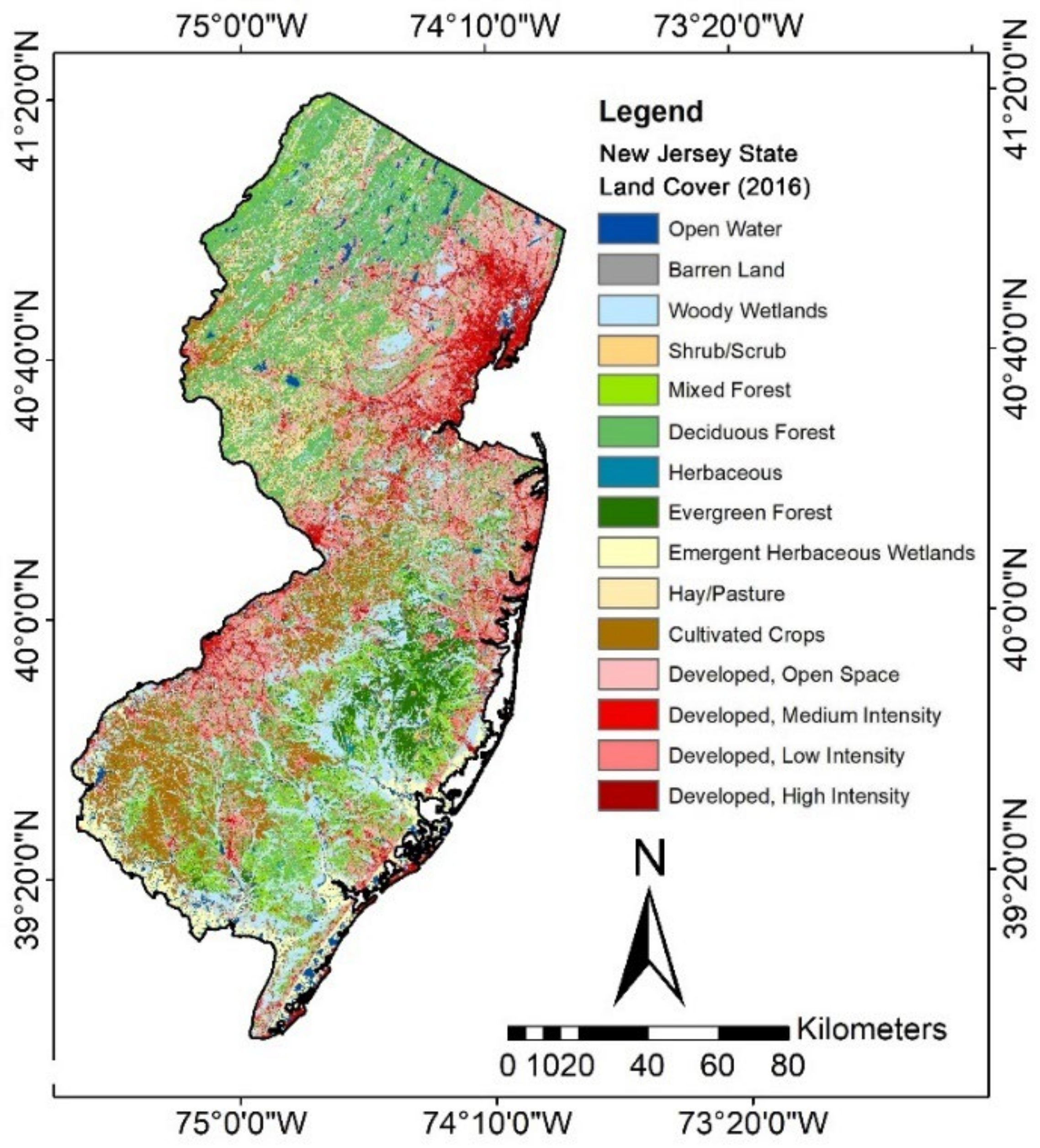
3.4. Land Use/Land Cover Change in New Jersey by Soil Order from 2001 to 2016
4. Significance of Results
4.1. Importance of Results for New Jersey’s GHG Emissions Inventory and Global Warming Response Act
4.2. Significance of Results in Broader Context
4.2.1. The Problem of Conflicts of Interest (COI) in Addressing Climate Change
- A.
- The many conflicts
- (1)
- Economic conflicts of interest for politicians. Many leaders who influence policy responding to climate change personally benefit from impeding action on climate change. GHGs are emitted by a host of business activities, such as coal and oil production and food production (e.g., the production of beef is a major source of GHGs). Indeed, almost all businesses are implicated because almost all businesses in some way use vehicles and power sources that burn fossil fuels. This paper measures the GHG emissions of yet another business activity: the disturbance of soil through development.
- (2)
- Intergenerational conflicts of interest. Morally, we should care as much about protecting the interests of our children and grandchildren, as our own interests; it would be immoral to destroy the world’s climate for our grandchildren, to further our own needs. However, decision-makers frequently are willing to forfeit the interests of future generations if preventing catastrophic climate change would cause even modest costs for the world’s current inhabitants. Although we should view the interests of our grandchildren as equal to our own, we do not; instead, the decision-makers’ personal interests are to favor the current generation because the decision-makers are themselves part of this generation. Leaders routinely favor their own interests over the interests of others who will live later, stating, for example, “who cares if Miami is six meters underwater in 100 years?” [36]. Just as COI cause decision-makers with links to oil companies improperly to favor oil companies over the general public, decision-makers with links to the current generation improperly favor this generation over all people, including people who will inherit the earth from us years from now.
- (3)
- Conflicts of interest between property owners and the public. Opposition to effective environmental programs can arise because of COI created by details of property law. For example, one might expect that owners of beachfront homes where the beach has eroded because of rising sea levels might support expensive public efforts to “renourish” the beaches by pumping in sand from the ocean floor. However, the property owners can instead oppose public renourishment projects in Florida and some other states, if the state’s law provides that the renourished beach will belong to the state. Because the state will now own the new strip of land next to the beach, and could conceivably sell it or build on it, the property owner will no longer own beachfront property [37].
- (4)
- Political conflicts for voters. The defining characteristic of many voters of a particular political party can be a belief that humans have not caused climate change [38]. To many members of such parties, to express a belief in anthropogenic climate change would be to deny one’s identity as a member of such a political party. A conflict of interest thus arises for some party members who have read and absorbed the consensus scientific literature that demonstrates that anthropogenic climate change exists. To express their belief in humans’ role in climate change would be to abandon their political party’s identity. For many, climate-change denial has become a creed of faith, not an issue of science. To deny this creed is to deny a fundamental tenet of the political party, to become an apostate, and to risk rejection from the community that, in part, defines itself by climate-change denial. This creates a COI that will cause even voters who secretly understand that humans cause climate change to express the opposite and to support political candidates who themselves deny climate change. Progress on reducing climate change is terminated by the conflict between some voters’ scientific understanding and the faith-creed of denial that they must express to remain members in good standing of their political community.
- (5)
- Political conflicts for politicians. To be elected, some politicians must adhere to the tenets of their party’s faith, including climate denial [39]. Because climate denialism is an essential requirement for membership in such a community, politicians recognize that public acceptance of the consensus on climate science would constitute political suicide. A political candidate who rejects this essential tenet of the party’s faith doctrine can expect rejection by the party’s faithful voters.
- (6)
- Conflicts for academic scientists. Conflicts of interest can also distort academic research [40]. Academic research can be a victim of COIs, where research is supported by industry. These conflicts can lead researchers to slant their results to benefit the industry that supports them. For example, scientists who are supported by oil companies may strain to produce results that deny anthropogenic climate change.
- (7)
- Conflicts in media. Conflicts abound in media [41] because any desire that conservative content providers’ might have to express the consensus existence of anthropogenic climate change conflicts with their incentive to express the climate change denial that is part of conservatives’ core beliefs [37]. As in academic science, some reporters and commentators may become climate-denial entrepreneurs, benefitting themselves and their employers by expressing to their conservative audience the climate-denial views that conservatives prefer—regardless of whether their expressed views conflict with their true views. These conflicts are not limited to conservative commentators. Liberal content providers may similarly shape their commentary to comply with liberal audiences’ preferences, even if the commentary conflicts with the content providers’ own views.
- (8)
- Conflicts due to competition among states. Although many states have the incentive to benefit their populations by reducing GHGs, they may also have the opposite tendency because of an incentive to attract industry and land developers from other states. For example, states often compete with each other to lure industry. To attract fossil-fuel companies, a state must have relaxed climate-change policies—even if these lax policies conflict with the stricter approach the state would otherwise pursue to protect its economy and its citizens’ health [42].
- (9)
- Conflicts between development and climate change. Our results demonstrate that development contributes to climate change by disturbing the soil and releasing GHGs. However, development also benefits the state by providing income, jobs, and taxes. A COI thus exists for NJ policymakers. Their desire to control climate change conflicts with their desire to promote development, which will help the economy in the short term. Because policymakers must appeal to voters in the short term, this conflict causes policymakers to sacrifice the state’s long-term interests in reducing climate change to policymakers’ interest in being reelected.
- B.
- What can be done?
4.2.2. The Role of Conflicts of Interest (COI) in Climate Change Litigation
5. Conclusions
Supplementary Materials
Author Contributions
Funding
Institutional Review Board Statement
Informed Consent Statement
Data Availability Statement
Conflicts of Interest
Glossary
| CF | Carbon footprint |
| ED | Ecosystem disservices |
| ES | Ecosystem services |
| EPA | Environmental Protection Agency |
| SC-CO2 | Social cost of carbon emissions |
| SDGs | Sustainable Development Goals |
| SOC | Soil organic carbon |
| SIC | Soil inorganic carbon |
| SOM | Soil organic matter |
| SSURGO | Soil Survey Geographic Database |
| STATSGO | State Soil Geographic Database |
| TSC | Total soil carbon |
| USDA | United States Department of Agriculture |
References
- EPA—United States Environmental Protection Agency, The Social Cost of Carbon. EPA Fact Sheet. 2016. Available online: https://19january2017snapshot.epa.gov/climatechange/social-cost-carbon_.html (accessed on 15 September 2021).
- New Jersey Statutes Annotated 26:2C-37. Global Warming Response Act. 2007. Available online: https://www.nj.gov/dep/aqes/docs/gw-responseact-07.pdf (accessed on 18 April 2022).
- New Jersey Executive Order No. 274. Available online: https://nj.gov/infobank/eo/056murphy/pdf/EO-274.pdf (accessed on 18 April 2022).
- Georgetown Climate Center. A Leading Resource for State and Federal Policy. 2022. Available online: https://www.georgetownclimate.org/adaptation/plans.html (accessed on 18 April 2022).
- United Nations. Paris Agreement. 2015. Available online: https://unfccc.int/sites/default/files/english_paris_agreement.pdf (accessed on 1 September 2021).
- Keestra, S.D.; Bouma, J.; Wallinga, J.; Tittonell, P.; Smith, P.; Cerdà, A.; Montanarella, L.; Quinton, J.N.; Pachepsky, Y.; Van der Putten, W.H.; et al. The significance of soils and soil science towards realization of the United Nations Sustainable Development Goals. Soil 2016, 2, 111–128. [Google Scholar] [CrossRef] [Green Version]
- New Jersey Department of Environmental Protection. 2018 Statewide Greenhouse Gas Emissions Inventory; New Jersey Department of Environmental Protection: Trenton, NJ, USA, 2019; pp. 1–21. [Google Scholar]
- Hill, R.; Rutkowski, M.M.; Lester, L.A.; Genievich, H.; Procopio, N.A. (Eds.) New Jersey Scientific Report on Climate Change, Version 1.0; New Jersey Department of Environmental Protection: Trenton, NJ, USA, 2020; p. 184. [Google Scholar]
- Mikhailova, E.A.; Groshans, G.R.; Post, C.J.; Schlautman, M.A.; Post, C.J. Valuation of total soil carbon stocks in the contiguous United States based on the avoided social cost of carbon emissions. Resources 2019, 8, 157. [Google Scholar] [CrossRef] [Green Version]
- Natural Resources Conservation Service. n.d. USDA. Downer—New Jersey State Soil. Available online: https://www.nrcs.usda.gov/Internet/FSE_DOCUMENTS/stelprdb1236981.pdf (accessed on 18 April 2022).
- Mikhailova, E.A.; Zurqani, H.A.; Post, C.J.; Schlautman, M.A.; Post, C.J. Soil diversity (pedodiversity) and ecosystem services. Land 2021, 10, 288. [Google Scholar] [CrossRef]
- Soil Survey Staff, Natural Resources Conservation Service, United States Department of Agriculture. n.d.a. Soil Survey Geographic (SSURGO) Database. Available online: https://nrcs.app.box.com/v/soils (accessed on 10 September 2021).
- The United States Census Bureau, TIGER/Line Boundary Shapefiles. 2018. Available online: https://www.census.gov/geographies/mapping-files/time-series/geo/tiger-line-file.2018.html (accessed on 10 September 2021).
- U.S. Bureau of the Census. Statistical Abstract of the United States: 1991; U.S. Bureau of the Census: Washington, DC, USA, 1991; p. 201. Available online: https://www.census.gov/library/publications/1991/compendia/statab/111ed.html (accessed on 10 December 2021).
- Hasse, J.E.; Lathrop, R.G. Measuring Urban Growth in New Jersey. A Report on Recent Land Development Patterns Utilizing the 1986-1995 NJ DEP Land Use/Land Cover Dataset; Rutgers University: New Brunswick, NJ, USA, 2001. [Google Scholar]
- Scharlemann, J.P.W.; Tanner, E.V.J.; Hiederer, R.; Kapos, V. Global soil carbon: Understanding and managing the largest terrestrial carbon pool. Carbon Manag. 2014, 5, 81–91. [Google Scholar] [CrossRef]
- Sanderman, J.; Hengl, T.; Fiske, G. Soil carbon debt of 12,000 years of human land use. Proc. Natl. Acad. Sci. USA 2017, 114, 9575–9580. [Google Scholar] [CrossRef] [PubMed] [Green Version]
- Lal, R. Societal value of soil carbon. J. Soil Water Conserv. 2014, 69, 186A–192A. [Google Scholar] [CrossRef] [Green Version]
- Roulet, N.T. Peatlands, carbon storage, greenhouse gases, and the Kyoto Protocol: Prospects and significance for Canada. Wetlands 2000, 20, 605–615. [Google Scholar] [CrossRef]
- Guo, Y.; Amundson, R.; Gong, P.; Yu, Q. Quantity and spatial variability of soil carbon in the conterminous United States. Soil Sci. Soc. Am. J. 2006, 70, 590–600. [Google Scholar] [CrossRef] [Green Version]
- Multi-Resolution Land Characteristics Consortium—MRLC. Available online: https://www.mrlc.gov/ (accessed on 1 September 2021).
- Groshans, G.R.; Mikhailova, E.A.; Post, C.J.; Schlautman, M.A.; Zhang, L. Determining the value of soil inorganic carbon stocks in the contiguous United States based on the avoided social cost of carbon emissions. Resources 2019, 8, 119. [Google Scholar] [CrossRef] [Green Version]
- ESRI—Environmental Systems Research Institute. ArcGIS Pro 2.6. Available online: https://pro.arcgis.com/en/pro-app/2.6/get-started/whats-new-in-arcgis-pro.htm (accessed on 1 September 2021).
- Mikhailova, E.A.; Groshans, G.R.; Post, C.J.; Schlautman, M.A.; Post, G.C. Valuation of soil organic carbon stocks in the contiguous United States based on the avoided social cost of carbon emissions. Resources 2019, 8, 153. [Google Scholar] [CrossRef]
- Ngoy, K.I.; Feng, Q.; Shebitz, D.J. Analyzing and predicting land use and land cover changes in New Jersey using multi-layer Perceptron-Markon chain model. Earth 2021, 2, 50. [Google Scholar] [CrossRef]
- Johnson, B.N.J. Environmentalists Go to Court to Force Murphy Administration to Adopt Climate Change Standards. Available online: https://www.nj.com/politics/2022/01/nj-environmentalists-go-to-court-to-force-murphy-administration-to-adopt-climate-change-standards.html (accessed on 10 June 2022).
- Soil Survey Staff, Natural Resources Conservation Service, United States Department of Agriculture. Photos of Soil Orders. Available online: https://www.nrcs.usda.gov/wps/portal/nrcs/detail/soils/edu/?cid=nrcs142p2_053588 (accessed on 20 September 2021).
- Bernardini, M. Rising seas could destroy millions of U.S. acres in decades. U.S. News, 8 September 2022. Available online: https://www.upi.com/Top_News/US/2022/09/08/Climate-Central-Maryland-Louisiana-North-Carolina-Texas/7951662676232/ (accessed on 13 September 2022).
- Fausset, R. Beach Houses on the Outer Banks Are Being Swallowed by the Sea. (14 May 2022). Available online: https://www.nytimes.com/2022/05/14/us/outer-banks-beach-houses-collapse.html (accessed on 1 June 2022).
- Watson, M.; Cullinane, S. Wildfire in Southern New Jersey grows to about 12,000 Acres. Available online: https://www.cnn.com/2022/06/20/weather/new-jersey-wildfire-wharton-state-forest/index.html (accessed on 10 June 2022).
- National Oceanic and Atmospheric Administration (NOAA). Available online: https://www.climate.gov/maps-data (accessed on 2 October 2022).
- Bion, J.; Antonelli, M.; Blanch, L.; Curtis, J.R.; Druml, C.; Du, B.; Machado, F.R.; Gomersall, C.; Hartog, C.; Levy, M. White paper: Statement on conflicts of interest. Intensive Care Med. 2018, 44, 1657–1668. [Google Scholar] [CrossRef] [PubMed]
- Bion, J.; Bellomo, R.; Finfer, S.; Myburgh, J.; Perner, A.; Reinhart, K. Comments: Response to correspondence from Van Aken and colleagues, and from Priebe, concerning our Open letter to the Executive Director of the European Medicines Agency concerning the licensing of hydroxyethyl starch solutions for fluid resuscitation. Br. J. Anaesth. 2014, 112, 595–600. [Google Scholar]
- Flavelle, C.; Tate, J. How Joe Manchin Aided Coal, and Earned Millions. Available online: https://www.nytimes.com/2022/03/27/climate/manchin-coal-climate-conflicts.html (accessed on 10 June 2022).
- Sneath, S. Louisiana Legislator Pushes Bills Benefiting the Oil and Gas Industry—And Her Husband. Available online: https://www.theguardian.com/environment/2022/may/06/sharon-hewitt-louisiana-senator-oil-gas-industry?CMP=oth_b-aplnews_d-1 (accessed on 10 June 2022).
- Vetter, D. “Who Cares If Miami Is 6 Meters Underwater In 100 Years?”: HSBC Executive’s Incendiary Climate Comments. Available online: https://www.forbes.com/sites/davidrvetter/2022/05/20/who-cares-if-miami-is-6-meters-underwater-in-100-years-hsbc-executives-incendiary-climate-comments/?sh=4b51e4ab590a (accessed on 10 June 2022).
- Meltz, R. Climate Change and Existing Law: A Survey of Legal Issues Past, Present, and Future. Available online: https://sgp.fas.org/crs/misc/R42613.pdf (accessed on 10 June 2022).
- Dietz, T. Political events and public views on climate change. Clim. Change 2020, 161, 1–8. [Google Scholar] [CrossRef] [PubMed]
- McCright, A.M.; Marquart-Pyatt, S.T.; Shwom, R.L.; Brechin, S.R.; Allen, S. Ideology, capitalism, and climate explaining public views about climate change in the United States. Energy Res. Soc. Sci. 2016, 21, 180–189. [Google Scholar] [CrossRef]
- Tollefson, J. Earth science wrestles with conflict-of-interest policies. Nature 2015, 522, 403–404. [Google Scholar] [CrossRef] [PubMed] [Green Version]
- Stecula, D.A.; Merkley, E. Framing climate change: Economics, ideology, and uncertainty in American news media content from 1988 to 2014. Front. Commun. 2019, 4, 6. [Google Scholar] [CrossRef] [Green Version]
- Basseches, J.A.; Bromley-Trujilli, R.; Boykoff, M.T.; Culhane, T.; Hall, G.; Healy, N.; Hess, D.J.; Hsu, D.; Krause, R.M.; Prechel, H. Climate policy confict in the U.S. states: A critical review and way forward. Clim. Change 2022, 170, 32. [Google Scholar] [CrossRef] [PubMed]
- Transparency International. Conflicts of Interest and Undue Influence in Climate Action: Putting a Stop to Corporate Efforts undermining Climate Policy and Decisions. Available online: https://images.transparencycdn.org/images/2021_ConflictsOfInterestClimateAction_PolicyBrief_EN.pdf (accessed on 9 October 2022).
- Weible, C.M.; Heikkila, T. Policy conflict framework. Policy Sci. 2017, 50, 23–40. [Google Scholar] [CrossRef]
- Doelle, M.; Seck, S. Loss and damage from climate change: from concept to remedy? Clim. Policy 2019, 20, 1–12. [Google Scholar]
- Strauss, B.H.; Orton, P.M.; Bitterman, K.; Buchanan, M.K.; Gilford, D.M.; Kopp, R.E.; Kulp, S.; Massey, C.; de Moel, H.; Vinogradov, S. Economic damages from Hurricane Sandy attributable to sea level rise caused by anthropogenic climate change. Nat. Commun. 2021, 12, 1–9. [Google Scholar] [CrossRef]
- Brown, S.; Miltner, E.; Cogger, C. Carbon Sequestration Potential in Urban Soils. In Carbon Sequestration in Urban Ecosystems; Springer: Dordrecht, The Netherlands, 2012; pp. 173–196. [Google Scholar]
- Andrews, C.J. Greenhouse gas emissions along the rural-urban gradient. J. Environ. Plan. Manag. 2008, 51, 847–870. [Google Scholar]


| Stocks | Ecosystem Services | |||
|---|---|---|---|---|
| Soil Order | General Characteristics and Constraints | Provisioning | Regulation/ Maintenance | Cultural |
| Slightly Weathered | ||||
| Entisols | Embryonic soils with an ochric epipedon | x | x | x |
| Inceptisols | Young soils with an ochric or umbric epipedon | x | x | x |
| Histosols | Organic soils with ≥20% organic carbon | x | x | x |
| Moderately Weathered | ||||
| Alfisols | Clay-enriched B horizon with B.S. ≥35% | x | x | x |
| Strongly Weathered | ||||
| Spodosols | Coarse-textured soils with albic and spodic horizons | x | x | x |
| Ultisols | Highly leached soils with B.S. <35% | x | x | x |
| Ownership (e.g., government, private, foreign, shared, single, etc.) | |||||
|---|---|---|---|---|---|
| Time (e.g., information disclosure, etc.) | Stocks/Source Attribution | Flows | Value | ||
| Biophysical Accounts (Science-Based) | Administrative Accounts (Boundary-Based) | Monetary Account(s) | Benefit(s)/ Damages | Total Value | |
| Soil extent: | Administrative extent: | Ecosystem good(s) and service(s): | Sector: | Types of value: | |
| Composite (total) stock: Total soil carbon (TSC) = Soil organic carbon (SOC) + Soil inorganic carbon (SIC) | |||||
| Past (e.g., post-development disclosures) Current (e.g., status) Future (e.g., pre-development disclosures) | Environment: | ”Avoided“ or ”realized” social cost of carbon (SC-CO2) emissions: | |||
| - Soil orders (Entisols, Inceptisols, Histosols, Alfisols, Spodosols, Ultisols). | - State (New Jersey); - County (21 counties). | - Regulation (e.g., carbon sequestration); - Provisioning (e.g., food production). | - Carbon gain (sequestration); - Carbon loss. | - $46 per metric ton of CO2 applicable for the year 2025 (2007 U.S. dollars with an average discount rate of 3% [1]). | |
| Conflicts of Interest (COI) | |||||
| County | Total Soil Area (km2) (%) | Degree of Weathering and Soil Development | |||||
|---|---|---|---|---|---|---|---|
| Slight | Moderate | Strong | |||||
| Entisols | Inceptisols | Histosols | Alfisols | Spodosols | Ultisols | ||
| 2016 Area (km2), (% of Total County Area) | |||||||
| Atlantic | 1395.3 (8) | 627.5 (45) | 106.1 (8) | 0.1 (0) | 0 (0) | 316.5 (23) | 345.2 (25) |
| Bergen | 350.2 (2) | 50.6 (14) | 47.9 (14) | 65.7 (19) | 97.6 (28) | 0 (0) | 88.4 (25) |
| Burlington | 2013.2 (12) | 650.6 (32) | 42.2 (2) | 159.2 (8) | 0 (0) | 168.7 (8) | 992.5 (49) |
| Camden | 457.6 (3) | 184.6 (40) | 47.3 (10) | 5.9 (1) | 0 (0) | 54.2 (12) | 165.7 (36) |
| Cape May | 603.9 (3) | 124.7 (21) | 181.7 (30) | 22.7 (4) | 0 (0) | 100.1 (17) | 174.7 (29) |
| Cumberland | 1184.1 (7) | 152.2 (13) | 207.8 (18) | 84.3 (7) | 0 (0) | 102.2 (9) | 637.7 (54) |
| Essex | 296.8 (2) | 67.0 (23) | 102.6 (35) | 2.6 (1) | 70.0 (24) | 0 (0) | 54.7 (18) |
| Gloucester | 742.6 (4) | 99.5 (13) | 20.1 (3) | 71.8 (10) | 0 (0) | 4.3 (1) | 546.9 (74) |
| Hudson | 41.1 (0.1) | 14.1 (34) | 19.2 (47) | 7.3 (18) | 0.5 (1) | 0 (0) | 0 (0) |
| Hunterdon | 1103.9 (6) | 14.6 (1) | 223.7 (20) | 0 (0) | 397.6 (36) | 0 (0) | 468.0 (42) |
| Mercer | 557.2 (3) | 55.1 (10) | 35.2 (6) | 0 (0) | 193.4 (35) | 0 (0) | 273.3 (49) |
| Middlesex | 718.0 (4) | 124.0 (17) | 62.5 (9) | 50.4 (7) | 84.7 (12) | 35.6 (5) | 360.6 (50) |
| Monmouth | 1172.3 (7) | 282.4 (24) | 107.8 (9) | 0.7 (0) | 0 (0) | 65.7 (6) | 715.8 (61) |
| Morris | 1124.4 (6) | 34.5 (3) | 455.6 (41) | 51.9 (5) | 140.0 (12) | 0 (0) | 442.3 (39) |
| Ocean | 1577.9 (9) | 773.7 (49) | 165.9 (11) | 10.5 (1) | 0 (0) | 294.2 (19) | 333.7 (21) |
| Passaic | 358.3 (2) | 56.2 (16) | 149.6 (42) | 12.7 (4) | 32.4 (9) | 0 (0) | 107.3 (30) |
| Salem | 795.3 (5) | 209.7 (26) | 0.3 (0) | 18.3 (2) | 0 (0) | 24.2 (3) | 542.8 (68) |
| Somerset | 776.7 (4) | 10.2 (1) | 127.2 (16) | 0 (0) | 420.2 (54) | 0 (0) | 219.1 (28) |
| Sussex | 1050.0 (6) | 37.4 (4) | 716.1 (68) | 39.3 (4) | 134.4 (13) | 0 (0) | 122.8 (12) |
| Union | 244.6 (1) | 72.8 (30) | 10.1 (4) | 4.2 (2) | 141.1 (58) | 0 (0) | 16.4 (7) |
| Warren | 811.4 (5) | 24.5 (3) | 473.7 (58) | 11.0 (1) | 199.2 (25) | 316.5 (0) | 103.0 (13) |
| Totals | 17,374.8 (100) | 3665.8 (21) | 3302.6 (19) | 618.6 (3) | 1911.2 (11) | 1165.6 (7) | 6711.1 (39) |
| Soil Order | SOC Content | SIC Content | TSC Content | SOC Value | SIC Value | TSC Value |
|---|---|---|---|---|---|---|
| Minimum—Midpoint—Maximum Values | Midpoint Values | |||||
| (kg m−2) | (kg m−2) | (kg m−2) | ($ m−2) | ($ m−2) | ($ m−2) | |
| Slightly Weathered | ||||||
| Entisols | 1.8–8.0–15.8 | 1.9–4.8–8.4 | 3.7–12.8–24.2 | 1.35 | 0.82 | 2.17 |
| Inceptisols | 2.8–8.9–17.4 | 2.5–5.1–8.4 | 5.3–14.0–25.8 | 1.50 | 0.86 | 2.36 |
| Histosols | 63.9–140.1–243.9 | 0.6–2.4–5.0 | 64.5–142.5–248.9 | 23.62 | 0.41 | 24.03 |
| Moderately Weathered | ||||||
| Alfisols | 2.3–7.5–14.1 | 1.3–4.3–8.1 | 3.6–11.8–22.2 | 1.27 | 0.72 | 1.99 |
| Strongly Weathered | ||||||
| Spodosols | 2.9–12.3–25.5 | 0.2–0.6–1.1 | 3.1–12.9–26.6 | 2.07 | 0.10 | 2.17 |
| Ultisols | 1.9–7.1–13.9 | 0.0–0.0–0.0 | 1.9–7.1–13.9 | 1.20 | 0.00 | 1.20 |
| County | Total SC-CO2 ($ = USD) | Degree of Weathering and Soil Development | |||||
|---|---|---|---|---|---|---|---|
| Slight | Moderate | Strong | |||||
| Entisols | Inceptisols | Histosols | Alfisols | Spodosols | Ultisols | ||
| Soil Organic Carbon (SOC), SC-CO2 ($ = USD) | |||||||
| Atlantic | 2.1 × 10⁹ | 8.5 × 10⁸ | 1.6 × 10⁸ | 1.6 × 10⁶ | 0 | 6.6 × 10⁸ | 4.1 × 10⁸ |
| Bergen | 1.9 × 10⁹ | 6.8 × 10⁷ | 7.2 × 10⁷ | 1.6 × 10⁹ | 1.2 × 10⁸ | 0 | 1.1 × 10⁸ |
| Burlington | 6.2 × 10⁹ | 8.8 × 10⁸ | 6.3 × 10⁷ | 3.8 × 10⁹ | 6.1 × 10⁴ | 3.5 × 10⁸ | 1.2 × 10⁹ |
| Camden | 7.7 × 10⁸ | 2.5 × 10⁸ | 7.1 × 10⁷ | 1.4 × 10⁸ | 0 | 1.1 × 10⁸ | 2.0 × 10⁸ |
| Cape May | 1.4 × 10⁹ | 1.7 × 10⁸ | 2.7 × 10⁸ | 5.4 × 10⁸ | 0 | 2.1 × 10⁸ | 2.1 × 10⁸ |
| Cumberland | 3.5 × 10⁹ | 2.1 × 10⁸ | 3.1 × 10⁸ | 2.0 × 10⁹ | 0 | 2.1 × 10⁸ | 7.7 × 10⁸ |
| Essex | 4.6 × 10⁸ | 9.0 × 10⁷ | 1.5 × 10⁸ | 6.1 × 10⁷ | 8.9 × 10⁷ | 0 | 6.6 × 10⁷ |
| Gloucester | 2.5 × 10⁹ | 1.3 × 10⁸ | 3.0 × 10⁷ | 1.7 × 10⁹ | 0 | 8.8 × 10⁶ | 6.6 × 10⁸ |
| Hudson | 2.2 × 10⁸ | 1.9 × 10⁷ | 2.9 × 10⁷ | 1.7 × 10⁸ | 6.9 × 10⁵ | 0 | 0 |
| Hunterdon | 1.4 × 10⁹ | 2.0 × 10⁷ | 3.4 × 10⁸ | 0 | 5.0 × 10⁸ | 0 | 5.6 × 10⁸ |
| Mercer | 7.0 × 10⁸ | 7.4 × 10⁷ | 5.3 × 10⁷ | 1.1 × 10⁶ | 2.5 × 10⁸ | 1.2 × 101 | 3.3 × 10⁸ |
| Middlesex | 2.1 × 10⁹ | 1.7 × 10⁸ | 9.4 × 10⁷ | 1.2 × 10⁹ | 1.1 × 10⁸ | 7.4 × 10⁷ | 4.3 × 10⁸ |
| Monmouth | 1.6 × 10⁹ | 3.8 × 10⁸ | 1.6 × 10⁸ | 1.6 × 10⁷ | 0 | 1.4 × 10⁸ | 8.6 × 10⁸ |
| Morris | 2.7 × 10⁹ | 4.7 × 10⁷ | 6.8 × 10⁸ | 1.2 × 10⁹ | 1.8 × 10⁸ | 0 | 5.3 × 10⁸ |
| Ocean | 2.6 × 10⁹ | 1.0 × 10⁹ | 2.5 × 10⁸ | 2.5 × 10⁸ | 0 | 6.1 × 10⁸ | 4.0 × 10⁸ |
| Passaic | 7.7 × 10⁸ | 7.6 × 10⁷ | 2.2 × 10⁸ | 3.0 × 10⁸ | 4.1 × 10⁷ | 0 | 1.3 × 10⁸ |
| Salem | 1.4 × 10⁹ | 2.8 × 10⁸ | 4.4 × 10⁵ | 4.3 × 10⁸ | 0 | 5.0 × 10⁷ | 6.5 × 10⁸ |
| Somerset | 1.0 × 10⁹ | 1.4 × 10⁷ | 1.9 × 10⁸ | 0 | 5.3 × 10⁸ | 0 | 2.6 × 10⁸ |
| Sussex | 2.4 × 10⁹ | 5.0 × 10⁷ | 1.1 × 10⁹ | 9.3 × 10⁸ | 1.7 × 10⁸ | 0 | 1.5 × 10⁸ |
| Union | 4.1 × 10⁸ | 9.8 × 10⁷ | 1.5 × 10⁷ | 1.0 × 10⁸ | 1.8 × 10⁸ | 0 | 2.0 × 10⁷ |
| Warren | 1.4 × 10⁹ | 3.3 × 10⁷ | 7.1 × 10⁸ | 2.6 × 10⁸ | 2.5 × 10⁸ | 0 | 1.2 × 10⁸ |
| Totals | 3.7× 10¹⁰ | 4.9× 10⁹ | 5.0× 10⁹ | 1.5× 10¹⁰ | 2.4× 10⁹ | 2.4× 10⁹ | 8.1× 10⁹ |
| County | Total SC-CO2 ($ = USD) | Degree of Weathering and Soil Development | |||||
|---|---|---|---|---|---|---|---|
| Slight | Moderate | Strong | |||||
| Entisols | Inceptisols | Histosols | Alfisols | Spodosols | Ultisols | ||
| Soil Inorganic Carbon (SIC), SC-CO2 ($ = USD) | |||||||
| Atlantic | 6.4 × 10⁸ | 5.1 × 10⁸ | 9.1 × 10⁷ | 2.8 × 10⁴ | 0 | 3.2 × 10⁷ | 0 |
| Bergen | 1.8 × 10⁸ | 4.2 × 10⁷ | 4.1 × 10⁷ | 2.7 × 10⁷ | 7.0 × 10⁷ | 0 | 0 |
| Burlington | 6.5 × 10⁸ | 5.3 × 10⁸ | 3.6 × 10⁷ | 6.5 × 10⁷ | 3.4 × 10⁴ | 1.7 × 10⁷ | 0 |
| Camden | 2.0 × 10⁸ | 1.5 × 10⁸ | 4.1 × 10⁷ | 2.4 × 10⁶ | 0 | 5.4 × 10⁶ | 0 |
| Cape May | 2.8 × 10⁸ | 1.0 × 10⁸ | 1.6 × 10⁸ | 9.3 × 10⁶ | 0 | 1.0 × 10⁷ | 0 |
| Cumberland | 3.5 × 10⁸ | 1.2 × 10⁸ | 1.8 × 10⁸ | 3.5 × 10⁷ | 0 | 1.0 × 10⁷ | 0 |
| Essex | 1.9 × 10⁸ | 5.5 × 10⁷ | 8.8 × 10⁷ | 1.1 × 10⁶ | 5.0 × 10⁷ | 0 | 0 |
| Gloucester | 1.3 × 10⁸ | 8.2 × 10⁷ | 1.7 × 10⁷ | 2.9 × 10⁷ | 0 | 4.3 × 10⁵ | 0 |
| Hudson | 3.1 × 10⁷ | 1.2 × 10⁷ | 1.7 × 10⁷ | 3.0 × 10⁶ | 3.9 × 10⁵ | 0 | 0 |
| Hunterdon | 4.9 × 10⁸ | 1.2 × 10⁷ | 1.9 × 10⁸ | 0 | 2.9 × 10⁸ | 0 | 0 |
| Mercer | 2.1 × 10⁸ | 4.5 × 10⁷ | 3.0 × 10⁷ | 1.9 × 10⁴ | 1.4 × 10⁸ | 0.6 | 0 |
| Middlesex | 2.4 × 10⁸ | 1.0 × 10⁸ | 5.4 × 10⁷ | 2.1 × 10⁷ | 6.1 × 10⁷ | 3.6 × 10⁶ | 0 |
| Monmouth | 3.3 × 10⁸ | 2.3 × 10⁸ | 9.3 × 10⁷ | 2.7 × 10⁵ | 0 | 6.6 × 10⁶ | 0 |
| Morris | 5.4 × 10⁸ | 2.8 × 10⁷ | 3.9 × 10⁸ | 2.1 × 10⁷ | 1.0 × 10⁸ | 0 | 0 |
| Ocean | 8.1 × 10⁸ | 6.3 × 10⁸ | 1.4 × 10⁸ | 4.3 × 10⁶ | 0 | 2.9 × 10⁷ | 0 |
| Passaic | 2.0 × 10⁸ | 4.6 × 10⁷ | 1.3 × 10⁸ | 5.2 × 10⁶ | 2.3 × 10⁷ | 0 | 0 |
| Salem | 1.8 × 10⁸ | 1.7 × 10⁸ | 2.5 × 10⁵ | 7.5 × 10⁶ | 0 | 2.4 × 10⁶ | 0 |
| Somerset | 4.2 × 10⁸ | 8.3 × 10⁶ | 1.1 × 10⁸ | 0 | 3.0 × 10⁸ | 0 | 0 |
| Sussex | 7.6 × 10⁸ | 3.1 × 10⁷ | 6.2 × 10⁸ | 1.6 × 10⁷ | 9.7 × 10⁷ | 0 | 0 |
| Union | 1.7 × 10⁸ | 6.0 × 10⁷ | 8.7 × 10⁶ | 1.7 × 10⁶ | 1.0 × 10⁸ | 0 | 0 |
| Warren | 5.8 × 10⁸ | 2.0 × 10⁷ | 4.1 × 10⁸ | 4.5 × 10⁶ | 1.4 × 10⁸ | 0 | 0 |
| Totals | 7.6× 10⁹ | 3.0× 10⁹ | 2.8× 10⁹ | 2.5× 10⁸ | 1.4× 10⁹ | 1.2× 10⁸ | 0 |
| County | Total SC-CO2 ($ = USD) | Degree of Weathering and Soil Development | |||||
|---|---|---|---|---|---|---|---|
| Slight | Moderate | Strong | |||||
| Entisols | Inceptisols | Histosols | Alfisols | Spodosols | Ultisols | ||
| Total Soil Carbon (TSC), SC-CO2 ($ = USD) | |||||||
| Atlantic | 2.7 × 10⁹ | 1.4 × 10⁹ | 2.5 × 10⁸ | 1.7 × 10⁶ | 0 | 6.9 × 10⁸ | 4.1 × 10⁸ |
| Bergen | 2.1 × 10⁹ | 1.1 × 10⁸ | 1.1 × 10⁸ | 1.6 × 10⁹ | 1.9 × 10⁸ | 0 | 1.1 × 10⁸ |
| Burlington | 6.9 × 10⁹ | 1.4 × 10⁹ | 1.0 × 10⁸ | 3.8 × 10⁹ | 9.5 × 10⁴ | 3.7 × 10⁸ | 1.2 × 10⁹ |
| Camden | 9.7 × 10⁸ | 4.0 × 10⁸ | 1.1 × 10⁸ | 1.4 × 10⁸ | 0 | 1.2 × 10⁸ | 2.0 × 10⁸ |
| Cape May | 1.7 × 10⁹ | 2.7 × 10⁸ | 4.3 × 10⁸ | 5.4 × 10⁸ | 0 | 2.2 × 10⁸ | 2.1 × 10⁸ |
| Cumberland | 3.8 × 10⁹ | 3.3 × 10⁸ | 4.9 × 10⁸ | 2.0 × 10⁹ | 0 | 2.2 × 10⁸ | 7.7 × 10⁸ |
| Essex | 6.5 × 10⁸ | 1.5 × 10⁸ | 2.4 × 10⁸ | 6.2 × 10⁷ | 1.4 × 10⁸ | 0 | 6.6 × 10⁷ |
| Gloucester | 2.7 × 10⁹ | 2.2 × 10⁸ | 4.7 × 10⁷ | 1.7 × 10⁹ | 0 | 9.3 × 10⁶ | 6.6 × 10⁸ |
| Hudson | 2.5 × 10⁸ | 3.1 × 10⁷ | 4.5 × 10⁷ | 1.7 × 10⁸ | 1.1 × 10⁶ | 0 | 0 |
| Hunterdon | 1.9 × 10⁹ | 3.2 × 10⁷ | 5.3 × 10⁸ | 0 | 7.9 × 10⁸ | 0 | 5.6 × 10⁸ |
| Mercer | 9.2 × 10⁸ | 1.2 × 10⁸ | 8.3 × 10⁷ | 1.1 × 10⁶ | 3.8 × 10⁸ | 1.3 × 101 | 3.3 × 10⁸ |
| Middlesex | 2.3 × 10⁹ | 2.7 × 10⁸ | 1.5 × 10⁸ | 1.2 × 10⁹ | 1.7 × 10⁸ | 7.7 × 10⁷ | 4.3 × 10⁸ |
| Monmouth | 1.9 × 10⁹ | 6.1 × 10⁸ | 2.5 × 10⁸ | 1.6 × 10⁷ | 0 | 1.4 × 10⁸ | 8.6 × 10⁸ |
| Morris | 3.2 × 10⁹ | 7.5 × 10⁷ | 1.1 × 10⁹ | 1.2 × 10⁹ | 2.8 × 10⁸ | 0 | 5.3 × 10⁸ |
| Ocean | 3.4 × 10⁹ | 1.7 × 10⁹ | 3.9 × 10⁸ | 2.5 × 10⁸ | 0 | 6.4 × 10⁸ | 4.0 × 10⁸ |
| Passaic | 9.7 × 10⁸ | 1.2 × 10⁸ | 3.5 × 10⁸ | 3.1 × 10⁸ | 6.4 × 10⁷ | 0 | 1.3 × 10⁸ |
| Salem | 1.6 × 10⁹ | 4.6 × 10⁸ | 6.9 × 10⁵ | 4.4 × 10⁸ | 0 | 5.2 × 10⁷ | 6.5 × 10⁸ |
| Somerset | 1.4 × 10⁹ | 2.2 × 10⁷ | 3.0 × 10⁸ | 0 | 8.4 × 10⁸ | 0 | 2.6 × 10⁸ |
| Sussex | 3.1 × 10⁹ | 8.1 × 10⁷ | 1.7 × 10⁹ | 9.5 × 10⁸ | 2.7 × 10⁸ | 0 | 1.5 × 10⁸ |
| Union | 5.8 × 10⁸ | 1.6 × 10⁸ | 2.4 × 10⁷ | 1.0 × 10⁸ | 2.8 × 10⁸ | 0 | 2.0 × 10⁷ |
| Warren | 2.0 × 10⁹ | 5.3 × 10⁷ | 1.1 × 10⁹ | 2.6 × 10⁸ | 4.0 × 10⁸ | 0 | 1.2 × 10⁸ |
| Totals | 4.5× 10¹⁰ | 8.0× 10⁹ | 7.8× 10⁹ | 1.5× 10¹⁰ | 3.8× 10⁹ | 2.5× 10⁹ | 8.0× 10⁹ |
| NLCD Land Cover Classes (LULC) | 2016 Total Area by LULC (km2) (Change in Area, 2001–2016, %) | Degree of Weathering and Soil Development | |||||
|---|---|---|---|---|---|---|---|
| Slight | Moderate | Strong | |||||
| Entisols | Inceptisols | Histosols | Alfisols | Spodosols | Ultisols | ||
| 2016 Area by Soil Order, km2 (Change in Area, 2001–2016, %) | |||||||
| Barren land | 53.9 (−11.9) | 17.3 (−11.9) | 3.6 (−14.8) | 7.2 (2.0) | 2.8 (−27.6) | 6.5 (−6.7) | 16.5 (−18.9) |
| Woody wetlands | 3180.1 (0.3) | 775.9 (0.3) | 885.9 (0.1) | 351.6 (2.2) | 152.1 (−0.9) | 342.5 (−0.2) | 672.1 (−0.7) |
| Shrub/Scrub | 124.1 (−23.4) | 30.0 (−23.4) | 13.0 (30.5) | 0.8 (−1.2) | 9.8 (−0.4) | 11.5 (−40.1) | 58.9 (−17.3) |
| Mixed forest | 1043.0 (−0.9) | 300.5 (−0.9) | 107.7 (−1.2) | 3.6 (−1.4) | 56.3 (−0.6) | 141.7 (−0.3) | 433.3 (−0.9) |
| Deciduous forest | 3582.8 (−7.4) | 340.2 (−7.4) | 1134.0 (−1.7) | 14.9 (−8.0) | 519.0 (−3.3) | 114.4 (−7.7) | 1460.2 (−4.3) |
| Herbaceous | 105.1 (9.5) | 33.3 (9.5) | 10.5 (54.5) | 3.4 (3.5) | 6.3 (7.2) | 11.6 (29.0) | 40.0 (−3.7) |
| Evergreen forest | 777.4 (−1.5) | 328.5 (−1.5) | 20.6 (−2.0) | 1.8 (−3.2) | 6.6 (−5.5) | 141.5 (0.6) | 278.3 (0.1) |
| Emergent herbaceous wetlands | 797.7 (−2.0) | 514.6 (−2.0) | 68.7 (−6.4) | 148.4 (−5.6) | 2.5 (−26.8) | 8.3 (−12.3) | 55.2 (−8.3) |
| Hay/Pasture | 827.3 (−15.5) | 17.7 (−15.5) | 252.7 (−6.3) | 2.6 (−28.8) | 280.1 (−8.9) | 2.0 (−12.0) | 272.3 (−10.7) |
| Cultivated crops | 1788.8 (−4.0) | 164.8 (−4.0) | 98.7 (3.3) | 7.0 (7.1) | 163.0 (3.8) | 82.2 (−2.6) | 1273.1 (−5.6) |
| Developed, open space | 351.1 (1.5) | 144.4 (1.5) | 42.1 (−88.4) | 4.0 (−89.4) | 25.9 (−92.7) | 27.3 (−75.3) | 107.4 (−89.0) |
| Developed, medium intensity | 1589.3 (12.2) | 355.6 (12.2) | 184.1 (13.3) | 22.4 (15.4) | 216.7 (15.8) | 105.7 (18.7) | 704.8 (27.3) |
| Developed, low intensity | 869.6 (4.4) | 274.2 (4.4) | 111.2 (4.0) | 13.9 (3.7) | 102.3 (5.1) | 57.7 (5.2) | 310.4 (9.8) |
| Developed, high intensity | 2284.6 (7.5) | 367.4 (7.5) | 370.4 (12.6) | 38.1 (24.3) | 367.9 (19.1) | 112.8 (10.7) | 1028.0 (27.8) |
| Soil Regulating Ecosystem Services in the State of New Jersey | |||||
|---|---|---|---|---|---|
| Degree of Weathering and Soil Development | |||||
| Slight 43% | Moderate 11% | Strong 46% | |||
| Entisols 21% | Inceptisols 19% | Histosols 3% | Alfisols 11% | Spodosols 7% | Ultisols 39% |
 |  |  |  |  |  |
| Social cost of soil organic carbon (SOC): $37.4 B | |||||
| $4.9 B | $5.0 B | $14.6 B | $2.4 B | $2.4 B | $8.1 B |
| 13% | 13% | 39% | 6% | 6% | 22% |
| Social cost of soil inorganic carbon (SIC): $7.6 B | |||||
| $3.0 B | $2.8 B | $253.5 M | $1.4 B | $116.5 M | $0.0 |
| 40% | 37% | 3% | 18% | 2% | 0% |
| Social cost of total soil carbon (TSC): $45.0 B | |||||
| $8.0 B | $7.8 B | $14.9 B | $3.8 B | $2.5 B | $8.0 B |
| 18% | 17% | 33% | 8% | 6% | 18% |
| Sensitivity to climate change | |||||
| Low | Low | High | High | Low | Low |
| SOC and SIC sequestration (recarbonization) potential | |||||
| Low | Low | Low | Low | Low | Low |
| NLCD Land Cover Classes (LULC) | Degree of Weathering and Soil Development | |||||
|---|---|---|---|---|---|---|
| Slight | Moderate | Strong | ||||
| Entisols | Inceptisols | Histosols | Alfisols | Spodosols | Ultisols | |
| Area Change, km2 (SC-CO2, $ = USD) | ||||||
| Developed, open space ($143.5 M) | 5.3 ($11.5 M) | 8.5 ($20.1 M) | 0.7 ($17.6 M) | 13.8 ($27.5 M) | 2.2 ($4.8 M) | 51.7 ($62.0 M) |
| Developed, medium intensity ($267.3 M) | 29.8 ($64.7 M) | 13.1 ($30.8 M) | 1.9 ($44.5 M) | 13.9 ($27.8 M) | 9.1 ($19.7 M) | 66.5 ($79.8 M) |
| Developed, low intensity ($176.5 M) | 14.9 ($32.2 M) | 7.1 ($16.7 M) | 0.8 ($19.4 M) | 10.6 ($21.1 M) | 5.2 ($11.3 M) | 63.2 ($75.8 M) |
| Developed, high intensity ($93.7 M) | 10.0 ($21.9 M) | 4.7 ($11.1 M) | 0.8 ($18.6 M) | 4.2 ($8.3 M) | 2.6 ($5.7 M) | 23.4 ($28.1 M) |
| Totals (364 km2 ($681.1 M) | 60.1 ($130.3 M) | 33.4 ($78.7 M) | 4.2 ($100.1 M) | 42.5 ($84.7 M) | 19.1 ($41.5 M) | 204.8 ($245.7 M) |
| County | Degree of Weathering and Soil Development | |||||
|---|---|---|---|---|---|---|
| Slight | Moderate | Strong | ||||
| Entisols | Inceptisols | Histosols | Alfisols | Spodosols | Ultisols | |
| Developed Area Increase between 2001 and 2016 (km2) (SC-CO2, $ = USD) | ||||||
| Atlantic | 9.9 ($21.4 M) | 0.03 ($78,588.0) | 0 | 0 | 3.4 ($7.4 M) | 7.8 ($9.3 M) |
| Bergen | 1.9 ($4.2 M) | 1.8 ($4.2 M) | 1.5 ($36.7 M) | 3.9 ($7.8 M) | 0 | 2.7 ($3.2 M) |
| Burlington | 2.3 ($4.9 M) | 0.3 ($787,900.8) | 0.06 ($1.6 M) | 0.01 ($19,900.0) | 1.3 ($2.7 M) | 32.6 ($39.2 M) |
| Camden | 2.4 ($5.3 M) | 0.8 ($1.9 M) | 0.01 ($240,300.0) | 0 | 0.6 ($1.3 M) | 5.7 ($6.9 M) |
| Cape May | 1.1 ($2.3 M) | 0.5 ($1.3 M) | 0.11 ($2.6 M) | 0 | 0.8 ($1.8 M) | 2.5 ($2.9 M) |
| Cumberland | 0.6 ($1.3 M) | 1.6 ($3.7 M) | 0.07 ($1.6 M) | 0 | 1.1 ($2.5 M) | 5.9 ($7.1 M) |
| Essex | 1.3 ($2.8 M) | 1.6 ($3.8 M) | 0.01 ($240,300.0) | 3.3 ($6.6 M) | 0 | 0.8 ($1.0 M) |
| Gloucester | 3.9 ($8.4 M) | 0.9 ($2.1 M) | 0.4 ($9.1 M) | 0 | 0 | 30.7 ($36.8 M) |
| Hudson | 0.7 ($1.6 M) | 0.8 ($1.9 M) | 0.4 ($9.1 M) | 0.01 ($19,900.0) | 0 | 0 |
| Hunterdon | 0.1 ($119,132.9) | 1.3 ($3.2 M) | 0 | 4.5 ($8.9 M) | 0 | 7.6 ($9.2 M) |
| Mercer | 1.0 ($2.1 M) | 0.3 ($616,351.8) | 0 | 4.0 ($8.0 M) | 0 | 18.0 ($21.6 M) |
| Middlesex | 3.3 ($7.3 M) | 1.6 ($3.7 M) | 1.1 ($26.0 M) | 2.5 ($4.9 M) | 1.3 ($2.9 M) | 26.6 ($32.0 M) |
| Monmouth | 6.9 ($15.0 M) | 3.7 ($8.7 M) | 0 | 0 | 2.4 ($5.3 M) | 33.4 ($40.1 M) |
| Morris | 1.2 ($2.6 M) | 9.2 ($21.6 M) | 0.4 ($9.4 M) | 2.7 ($5.3 M) | 0 | 20.2 ($24.3 M) |
| Ocean | 21.5 ($46.7 M) | 1.0 ($2.5 M) | 0.2 ($4.9 M) | 0 | 8.8 ($19.1 M) | 15.0 ($18.0 M) |
| Passaic | 0.9 ($2.0 M) | 2.2 ($5.1 M) | 0.12 ($2.8 M) | 4.3 ($8.7 M) | 0 | 0.6 ($721,668.4) |
| Salem | 1.2 ($2.5 M) | 0 | 0.01 ($240,300.0) | 0 | 0.03 ($54,684.0) | 2.3 ($2.8 M) |
| Somerset | 0.5 ($1.0 M) | 2.0 ($4.7 M) | 0 | 12.9 ($25.6 M) | 0 | 6.6 ($7.9 M) |
| Sussex | 1.0 ($2.2 M) | 4.3 ($9.3 M) | 0 | 2.1 ($2.2 M) | 0 | 0.8 ($942,869.9) |
| Union | 1.1 ($2.4 M) | 0.1 ($165,200.0) | 0.01 ($240,300.0) | 1.3 ($2.6 M) | 0 | 0.1 ($108,000.0) |
| Warren | 0.4 ($779,246.7) | 1.2 ($2.8 M) | 0 | 5.2 ($10.3 M) | 0 | 0.3 ($405,000.2) |
| 389.7 km2 ($722.2 M) | 63.1 ($136.8 M) | 35.2 ($82.1 M) | 4.4 ($104.8 M) | 46.7 ($90.9 M) | 19.9 ($43.1 M) | 220.4 ($264.5 M) |
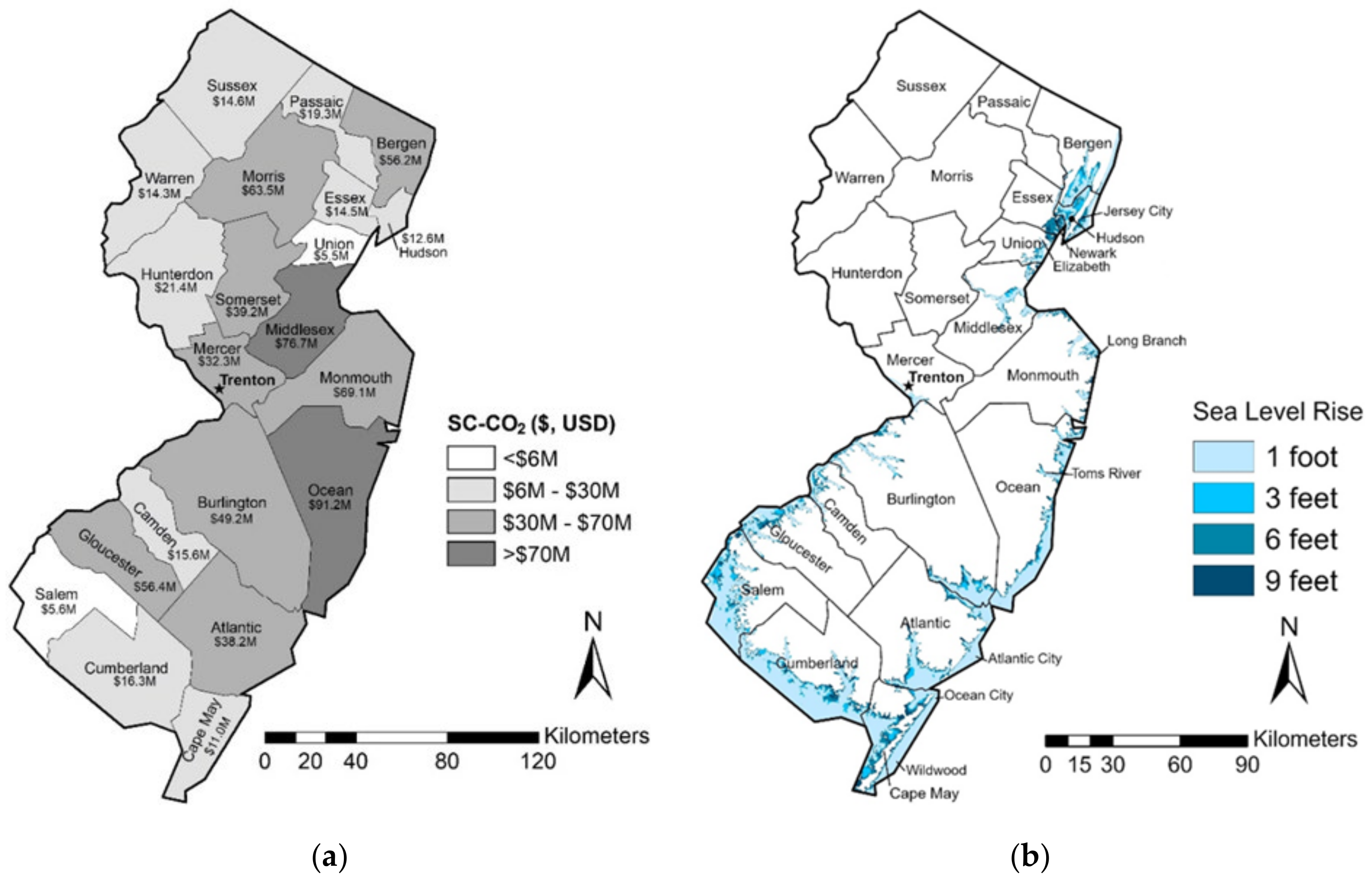
| County (Affected by Sea Rise) | County Area Loss due to Sea Rise (% County Area) | |||
|---|---|---|---|---|
| 1 Foot | 3 Feet | 6 Feet | 9 Feet | |
| Atlantic | 11.9 | 13.5 | 15.7 | 17.8 |
| Bergen | 6.3 | 8.7 | 11.7 | 13.2 |
| Burlington | 3.9 | 4.8 | 6.0 | 7.2 |
| Camden | 2.7 | 3.2 | 4.8 | 6.0 |
| Cape May | 32.9 | 37.9 | 45.1 | 53.8 |
| Cumberland | 24.0 | 26.9 | 30.5 | 33.5 |
| Essex | 1.0 | 1.0 | 4.0 | 7.9 |
| Gloucester | 6.2 | 7.5 | 9.7 | 11.7 |
| Hudson | 22.3 | 27.1 | 42.0 | 54.2 |
| Mercer | 1.7 | 1.8 | 2.0 | 2.1 |
| Middlesex | 2.8 | 3.9 | 5.1 | 6.4 |
| Monmouth | 1.7 | 2.0 | 3.0 | 4.1 |
| Ocean | 9.3 | 10.7 | 12.8 | 14.5 |
| Passaic | 0.1 | 0.1 | 0.1 | 0.2 |
| Salem | 18.5 | 22.9 | 27.6 | 31.2 |
| Union | 2.1 | 2.7 | 5.0 | 8.0 |
| NLCD Land Cover Classes (LULC) | 2016 Total Area by LULC (%) | Degree of Weathering and Soil Development | |||||
|---|---|---|---|---|---|---|---|
| Slight | Moderate | Strong | |||||
| Entisols | Inceptisols | Histosols | Alfisols | Spodosols | Ultisols | ||
| 2016 Area by Soil Order, % from Total Area in each LULC | |||||||
| Barren land | 0.3 | 32.1 | 6.8 | 13.4 | 5.1 | 12.0 | 30.6 |
| Woody wetlands | 18.3 | 24.4 | 27.9 | 11.1 | 4.8 | 10.8 | 21.1 |
| Shrub/Scrub | 0.7 | 24.2 | 10.5 | 0.6 | 7.9 | 9.3 | 47.5 |
| Mixed forest | 6.0 | 28.8 | 10.3 | 0.3 | 5.4 | 13.6 | 41.5 |
| Deciduous forest | 20.6 | 9.5 | 31.7 | 0.4 | 14.5 | 3.2 | 40.8 |
| Herbaceous | 0.6 | 31.7 | 10.0 | 3.3 | 6.0 | 11.1 | 38.0 |
| Evergreen forest | 4.5 | 42.3 | 2.6 | 0.2 | 0.9 | 18.2 | 35.8 |
| Emergent herbaceous wetlands | 4.6 | 64.5 | 8.6 | 18.6 | 0.3 | 1.0 | 6.9 |
| Hay/Pasture | 4.8 | 2.1 | 30.5 | 0.3 | 33.9 | 0.2 | 32.9 |
| Cultivated crops | 10.3 | 9.2 | 5.5 | 0.4 | 9.1 | 4.6 | 71.2 |
| Developed, open space | 2.0 | 41.1 | 12.0 | 1.1 | 7.4 | 7.8 | 30.6 |
| Developed, medium intensity | 9.1 | 22.4 | 11.6 | 1.4 | 13.6 | 6.7 | 44.3 |
| Developed, low intensity | 5.0 | 31.5 | 12.8 | 1.6 | 11.8 | 6.6 | 35.7 |
| Developed, high intensity | 13.1 | 16.1 | 16.2 | 1.7 | 16.1 | 4.9 | 45.0 |
Publisher’s Note: MDPI stays neutral with regard to jurisdictional claims in published maps and institutional affiliations. |
© 2022 by the authors. Licensee MDPI, Basel, Switzerland. This article is an open access article distributed under the terms and conditions of the Creative Commons Attribution (CC BY) license (https://creativecommons.org/licenses/by/4.0/).
Share and Cite
Mikhailova, E.A.; Lin, L.; Hao, Z.; Zurqani, H.A.; Post, C.J.; Schlautman, M.A.; Post, G.C.; Shepherd, G.B. Conflicts of Interest and Emissions from Land Conversions: State of New Jersey as a Case Study. Geographies 2022, 2, 669-690. https://doi.org/10.3390/geographies2040041
Mikhailova EA, Lin L, Hao Z, Zurqani HA, Post CJ, Schlautman MA, Post GC, Shepherd GB. Conflicts of Interest and Emissions from Land Conversions: State of New Jersey as a Case Study. Geographies. 2022; 2(4):669-690. https://doi.org/10.3390/geographies2040041
Chicago/Turabian StyleMikhailova, Elena A., Lili Lin, Zhenbang Hao, Hamdi A. Zurqani, Christopher J. Post, Mark A. Schlautman, Gregory C. Post, and George B. Shepherd. 2022. "Conflicts of Interest and Emissions from Land Conversions: State of New Jersey as a Case Study" Geographies 2, no. 4: 669-690. https://doi.org/10.3390/geographies2040041