Mapping Construction Costs at the National Level

Abstract

The construction industry relies on construction cost indexes to prepare cost estimate benchmarks and develop cost estimates. Subsequently, government agencies, non-profit organizations, and private companies routinely publish construction cost indexes for cities. Currently, all construction cost indexes are released in a tabular format for 649 cities across the conterminous United States, which is not effective in illustrating construction cost variations at the national level. This study explored the utility of various established interpolation methods and mapping techniques to visualize construction cost indexes at the national level. Geovisualization techniques such as thematic mapping provide a visual representation of construction cost data in addition to traditional tabular formats. This study explored the utility of Thiessen polygon and inverse distance weighted (IDW) methods to create thematic maps which can be used to interactively visualize construction costs at the national level. A qualitative comparison revealed that the IDW method can produce the most intuitive, interactive, and continuous surface maps to identify dynamic and previously unrecognized patterns. These continuous surface maps allow construction practitioners and academics, real estate developers, and the public to locate the geographic proximity of high or low construction costs while cost change maps allow investors and businesses to identify patterns in changing construction costs over a certain period. This work contributes to the body of knowledge by introducing interpolated maps for visualizing any construction cost-related indexes at a large scale such as the national level.

1. Introduction

The construction industry plays a key role in a country’s economy, in addition to producing physical structures that increase productivity and quality of life [1,2]. Construction is one of the largest industries in the United States, and it is the country’s largest single production economic activity in terms of dollar value of the output produced within the borders of the nation [3]. According to the Bureau of Labor Statistics of the United States, the industry employs 8.3 million people and represents 5 percent of the workforce [4].

Therefore, construction is an important sector that contributes greatly to a nation’s economic growth. Consequently, construction costs are a critical indicator of economic conditions because the construction market tends to follow the condition of the overall economy [5]. Generally, construction costs tend to decrease in times of recession because demand for new construction is low, while construction costs tend to increase in times of economic boom because demand is high [5].

In the construction industry, one of the common practices is to conduct project feasibility studies to assess the viability of a construction project prior to site acquisition or entering into a building commitment [6]. It should be noted that early and accurate construction cost forecasting is needed in such studies. Such forecasting, which is commonly known as construction cost estimating, is the process of forecasting the cost of building a physical structure such as a building or a bridge. Construction cost estimating can be used to assist project stakeholders in many ways, including, but not limited to, predicting costs, setting a budget, and managing design to meet budget restrictions [6].

In general, construction cost estimates are developed by using historical cost data and applying various adjustment factors to reflect the local costs of labor, material, equipment, project size, and project complexity. For example, the most common practice for estimating the total cost to construct a project at a specific location is to adjust standardized costs by applying a construction cost index for that location. That being said, the construction industry relies on location-based construction cost indexes to prepare cost estimate benchmarks and develop cost estimates. Subsequently, government agencies, non-profit organizations, and even private companies routinely (i.e., weekly, monthly, semi-annually, or annually) publish location-based construction cost indexes on a national scale to assist the construction industry with cost estimation. These cost indexes are also commonly used by investors and businesses to evaluate economic health and adjust their perspectives on economic growth and profitability.

In the United States, the most widely used location-based construction cost index is the RSMeans city cost index (CCI).

Table 1. City cost indexes for cities in the states of Alabama and Arizona.

State	City	Material	Installation	Total
Alabama	Birmingham	97.4	75.2	87.6
	Tuscaloosa	96.0	60.2	80.2
	Jasper	96.3	58.5	79.6
	Decatur	96.0	61.8	80.9
	Huntsville	96.0	70.1	84.6
	Gadsden	95.9	59.2	79.7
	Montgomery	97.1	58.3	80.0
	Anniston	95.2	67.0	82.8
	Dothan	95.9	53.7	77.3
	Evergreen	95.4	55.6	77.8
	Mobile	97.1	67.4	84.0
	Selma	95.6	53.5	77.0
	Phoenix City	96.4	57.2	79.1
	Butler	95.8	53.9	77.3
Arizona	Phoenix	99.9	74.6	88.7
	Mesa/Tempe	99.4	64.4	83.9
	Globe	99.5	60.5	82.3
	Tucson	98.2	69.9	85.7
	Show Low	99.6	61.6	82.8
	Flagstaff	101.6	70.4	87.9
	Prescott	99.1	61.1	82.4
	Kingman	97.2	67.9	84.3
	Chambers	97.3	61.8	81.6

shows the 2010 CCI for cities in the states of Alabama and Arizona as an example; although, the CCI information is available for all 50 U.S. states. It should be noted that the construction cost for a city includes two components: material costs and installation costs (including both labor costs and equipment rental costs). The “Total” is the weighted average composite index, which reflects both material and installation costs, and it is the index referred to as the CCI. The weighted average for a city is a total of the divisional components weighted to reflect typical usage, but it does not include the productivity variations between trades or cities [7]. Additionally, the CCI does not take into account factors such as managerial efficiency, local competitive conditions, construction automation, restrictive union practices, unique local requirements, and local building codes [7].

It should be noted that CCI values are also available for cities in U.S. territories and Canada. The CCI is a percentage ratio of the construction cost of a given city to the national average construction cost at a stated period of time [7]. That said, these index figures represent relative construction factors (i.e., multipliers) for materials, installation, and total costs (i.e., CCI) at a specific location when compared to the national average, which is set at 100. The construction costs of thirty major U.S. cities (e.g., New York and Los Angeles) are used to calculate the national average. For example, if the CCI value of a city is 80 in 2005, it indicates the construction cost of that city is 80% of the national average in the year 2005.

Currently, all construction cost indexes from RSMeans are released in a tabular format, lacking a straightforward illustration of the variation of construction costs at the national level. In addition, construction cost indexes are not available for all locations across the United States. For example, in the conterminous United States (excluding the states of Hawaii and Alaska), RSMeans routinely surveys 649 cities out of over 19,000 cities listed by the U.S. Census Bureau, which means that less than 4% of U.S. cities have been surveyed on a regular basis [8].

Maps provide an effective representation of data where the individual values are traditionally contained in a matrix because maps are an intuitive and user-friendly medium for representing information visually [9,10]. Due to these unique features, maps hold the potential to more effectively and efficiently visualize construction costs at the national level. It should be noted that map creation involves the process of effectively and efficiently visualizing geospatial information known as geovisualization [11]. Traditional maps can be characterized as being static, which limits their exploratory capability. Geovisualization, on the other hand, leverages a set of tools and techniques (e.g., internet mapping) to permit the creation of more interactive and dynamic maps [11].

There have been steadily growing research interests and efforts in the cartographic and geographic information science community for the effective and efficient visualization of myriad geospatial data through the use of a variety of new technologies and techniques for the purposes of geographic knowledge discovery, information sharing, and decision-making processes [12]. Over the past four decades, remote sensing missions (e.g., satellite imagery) and field survey work have exponentially increased the volumes of geospatial data available [13]. In this context, geovisualization is both a process for leveraging these geospatial data to meet scientific and societal needs, and a research field that develops visual methods and tools to support a wide range of geospatial data applications [14].

In recent years, researchers and practitioners have found a variety of creative ways to use new technologies and techniques to advance geovisualization. However, challenges still remain. Some of the challenges include the presentation of multivariate geospatial data, visualization–computation integration, user interface–device integration, and usability and cognitive issues [11]. All these challenges can be attributed to a lack of methods for transforming the ever-increasing geospatial data into information and for combining information from diverse sources to construct knowledge [11].

Currently, there are no national-level construction cost maps available due to the lack of data for unsurveyed cities and geovisualization methods. From the perspective of the survey, it is impossible to survey every single city’s construction cost due to limited resources (e.g., money and manpower). To estimate the construction cost for a city that does not have a CCI, the widely adopted method in the construction industry is to use the nearest (in terms of geographic proximity) city’s CCI.

From the perspective of geovisualization, a review of the literature revealed that methods for visualizing the CCI are limited and present a significant gap in the research. Several recent studies have revealed that several interpolation methods can be effectively used to estimate the CCI for unknown locations [15,16]. These methods include the nearest neighbor (NN) method, the conditional nearest neighbor (CNN) method, and the inverse distance weighted (IDW) method. The NN method is the most widely adopted method in the construction industry to estimate the CCI for unsurveyed cities. The other two methods, CNN and IDW, have been identified by previous studies as better alternatives when compared to NN. The CNN method is very similar to the NN method, but state boundaries play a role in determining the nearest neighbor in CNN. In other words, when using the CCN method, a city’s nearest neighbor has to be within the same state. The IDW method uses the weighted average of a known location’s CCI within the neighborhood to estimate the CCI of an unknown location. More details regarding NN, CNN, and IDW are discussed in the methodology section.

These three methods hold the potential to effectively and efficiently visualize CCI values at the national level via a series of maps to reveal spatial-temporal patterns that have traditionally been impossible to reveal by a tabular format. This is because, fundamentally, the CCI is geospatial data, i.e., a combination of location information (coordinates that define a specific feature, in this case, a specific city); attribute information (the characteristics that define a specific feature, in this case, a specific city); and temporal information (when the data are being collected, edited, and distributed). The attribute information is essentially the construction cost information that describes a city with a specific location. The intellectual significance of this research lies in exploring the utility of three geovisualization methods, including NN, CNN, and IDW, to permit visualization of the CCI at the national level. Unlike the traditional presentation of a CCI in a tabular format, this study visualizes CCI data through a series of maps.

All the aforementioned methods, including NN, CNN, and IDW, are spatial interpolation methods that can be used to produce maps that illustrate the variation of national-level construction costs over time. These maps can be considered “heatmaps”: a grid composed of pixels with different colors, each of which corresponds to a data value; the hotter the color is, the higher the pixel value is [17]. This study explores the utility of NN, CNN, and IDW methods for mapping construction costs at the national level. Specifically, the intent of this study is to examine whether construction cost data can be mapped from NN, CNN, and IDW methods to exhibit their spatial-temporal patterns, and if so, to determine which method produces the most intuitive and interactive maps to assist construction practitioners and academics, real estate developers, investors and businesses, and the public in identifying dynamic and previously unrecognized patterns.

2. Materials and Methods

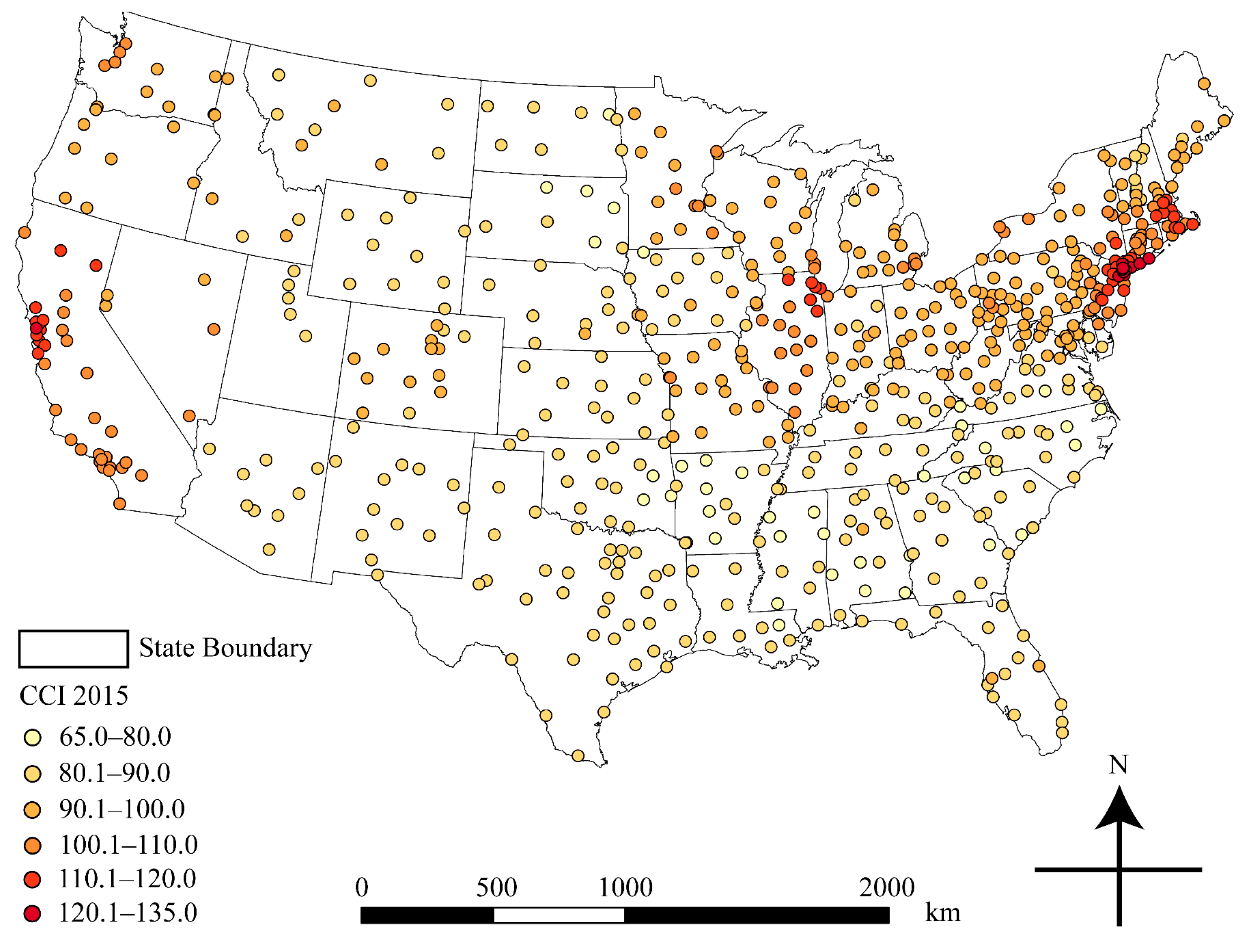
2.1. Construction Cost Data Collection

Construction material, labor, and equipment costs are factors used for calculating the CCI. However, it should be noted that other elements such as weather, climate, transportation, and labor productivity are not considered in the CCI estimates. The CCI is surveyed, updated, and published on an annual basis. For the 649 cities surveyed across the conterminous United States, the CCI values from 2004 to 2015 were obtained from RSMeans. This study did not use the latest CCI data because the data used are irrelevant since this study is focused on demonstrating how to use NN, CNN, and IDW methods to create construction cost maps at the national level.

These 2004 to 2015 CCI values were tabular-joined with a standard GIS point shapefile of cities obtained from ESRI [18] and saved for later processing. It should be noted that the cities in the states of Hawaii and Alaska were excluded because they do not have neighboring states to interpolate CCI values with the NN and IDW methods. This could be a future research topic which focuses on mapping construction costs at the state level.

Figure 1 shows the locations of these 649 cities using a color scheme to indicate each city’s CCI value category in 2015. CCI values are represented via increasingly warm color hues (e.g., red color), which are prevalent in the construction field [19]. Users can identity a city’s CCI from one of the seven categories as indicated in Figure 1. However, it is not possible for users to identify CCI values for cities that are not listed among the 649 cities.

Previous studies have proven that cities with CCI values are spatially auto-correlated [15,16], meaning that it is valid to perform interpolation for locations that do not have CCI values. As mentioned in the previous section, three methods, including NN, CNN, and IDW were selected as the interpolation techniques for estimating CCI values for cities not currently included in the index database.

2.2. Interpolation Methods

Interpolation allows users to estimate values at locations where they have not yet been measured [20]. These methods are commonly used when samples are limited, lost, incomplete, or when previously collected data may be dated and inaccurate [20]. When using the NN method, users select the value of the nearest surveyed city (in terms of Euclidean or linear distance, not actual travel distance over a road network) to estimate the CCI value for an unsurveyed location. The Thiessen polygon method was used to identify a zone closest to each of the 649 CCI sites (Figure 2); cities within the same zone were then assigned the same CCI value. However, when compared with alternative proximity-based interpolation methods such as CNN and IDW, NN has been proven to be less accurate [16].

The CNN method improves upon the NN method by selecting the value of the nearest surveyed city within the same state to estimate the CCI for an unsurveyed city. A previous study concluded that the CNN method outperforms the NN method in terms of accuracy because state boundaries are used concurrently with geographic proximity to select the nearest neighbor [16]. In addition, the CNN method is also the best method for creating a rough surface map of CCI (i.e., classified choropleth map) [16]. Figure 3 shows the use of the Thiessen polygon and state boundaries to implement the CNN method.

The IDW method is one of the most frequently used deterministic models in interpolation. This method evolved from the assumption that the attribute value of an unsurveyed point is the weighted average of known values within the neighborhood, and that those weights are inversely related to the distances between the unsurveyed and surveyed locations [21]. IDW is the best method for creating a smooth surface map of the CCI (i.e., stretched raster map) [16]. Equation (1) shows the algorithm of the IDW interpolation method. With IDW, values for unsurveyed points, Z_j, are estimated by:

$$Z_j=\frac{{{\displaystyle \sum }}_i\frac{Z_i}{d_{ij}^n}}{{{\displaystyle \sum }}_i\frac{1}{d_{ij}^n}}$$

(1)

where d_ij is the distance from known point i to unknown point j, Z_i is the value for the known point i, and n is a user defined exponent, which controls how quickly a point’s influence decreases with distance [20]. According to the previous study, a value of 2 should be used for n, and the search radius should be limited to 10 neighboring points [16]. The output cell size (grid resolution) should be 1 km. Figure 4 shows an interpolated surface map produced by the IDW method.

2.3. Selection of Interpolation Method for Mapping

As shown in Figure 2 and Figure 3, both the NN and CNN methods can estimate CCI values for all cities at the national level. The color variation at the polygon level in these maps produces two-dimensional (2D) choropleth maps, which are only able to represent class membership per polygon [22]. If actual values are not available for reference units, unsurveyed cities can only be compared with class range values [22], which are very difficult if not impossible to interpret. A lack of variation within the polygons makes it more difficult for the viewers to assess the CCI values for unsurveyed cities, which can lead to difficulty in identifying any general patterns. Additionally, both NN and CCN methods will produce rough surfaces for the interpolated CCI values, which means that CCI values will change suddenly from one value to the next across certain boundaries creating a rough surface with jump discontinuities [16]. These discontinuities may greatly hinder CCI distribution pattern identification at the national level.

IDW methods, as shown in Figure 4, can also show CCI values for all cities at the national level. Previous studies have shown that the IDW method provides a more accurate interpolation of the CCI values; however, mathematically, IDW is slow and difficult to calculate [16]. However, modern spatial computing technologies have greatly alleviated this challenge. In addition, the IDW method involves many algorithm parameters and users need to identify the most appropriate ones to create the most accurate interpolation surface [16]. Unlike the polygon-based NN and CNN interpolation methods, IDW creates a smoother raster surface that can be used to assist in the comprehension of demographic or economic data more effectively than polygon-based, classified choropleth maps [22]. Therefore, the IDW method generally produces smooth surface maps that are more intuitive, which aid viewers in identifying overall, dynamic, and previously unrecognized patterns. Therefore, the authors decided to use IDW to create maps for CCI values at the national level to reveal spatial-temporal patterns more effectively.

Table 2. Advantages and disadvantages of each interpolation method.

Methods	Advantages	Disadvantages
NN	Fast and easy to calculate	Less accurate
	Widely adopted by the construction industry to conduct cost estimates	Lack of variation within the polygon; no use of state boundary
	Can estimate CCI values for all cities at the national level	Rough surfaces for the interpolated CCI values
CNN	More accurate	Slow and difficult to calculate
	Consider state policies’ and regulations’ impact on cost variation	Lack of variation within the polygon
	Can estimate CCI values for all cities at the national level	Rough surfaces for the interpolated CCI values
IDW	More accurate	Slow and difficult to calculate
	Smooth surfaces for the interpolated CCI values which provide a more intuitive look to identify patterns	More parameters such as power to consider and test prior to deployment
	Can estimate CCI values for all cities at the national level	Unable to consider state policies’ impact on cost variation

summarizes the advantages and disadvantages of the aforementioned methods.

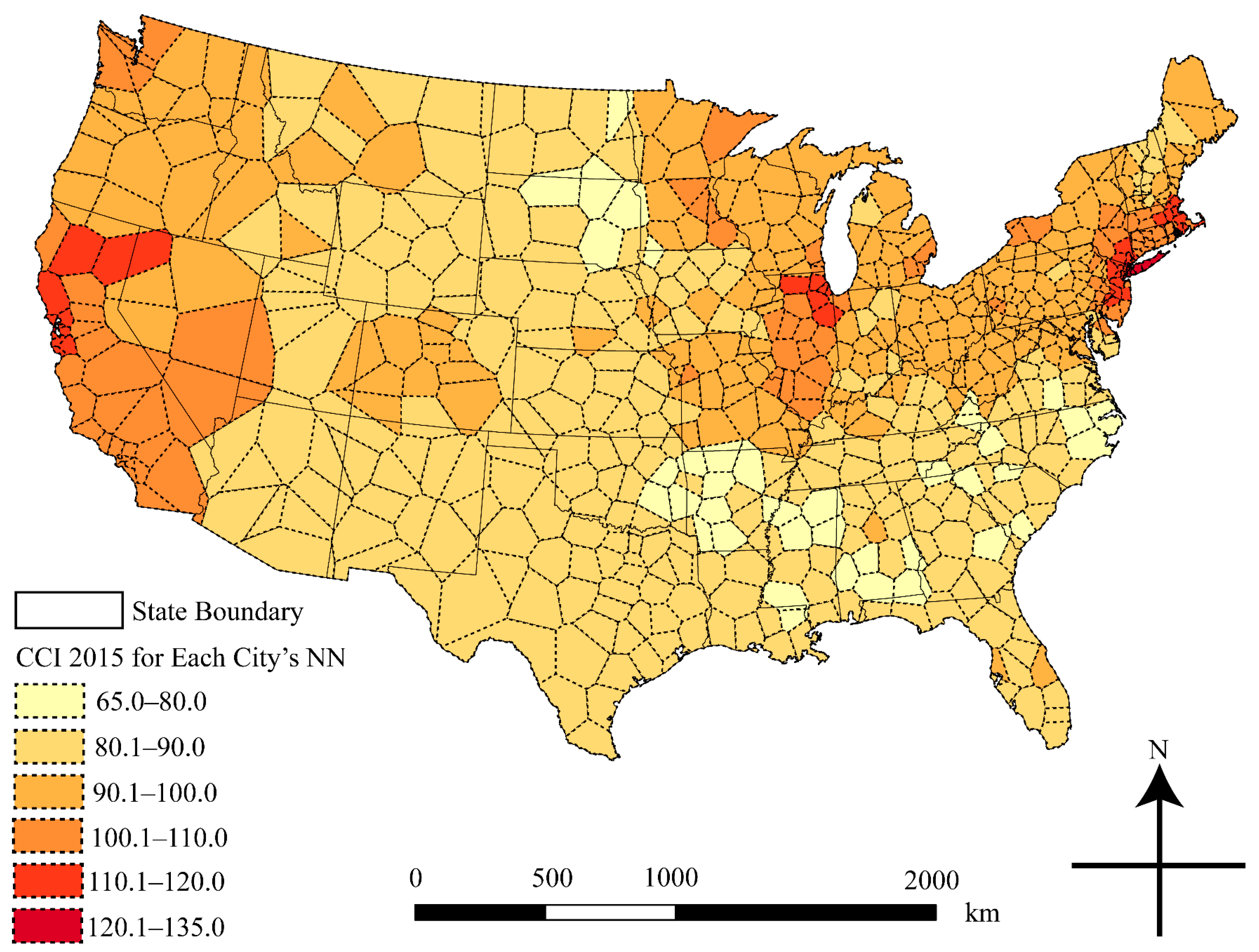
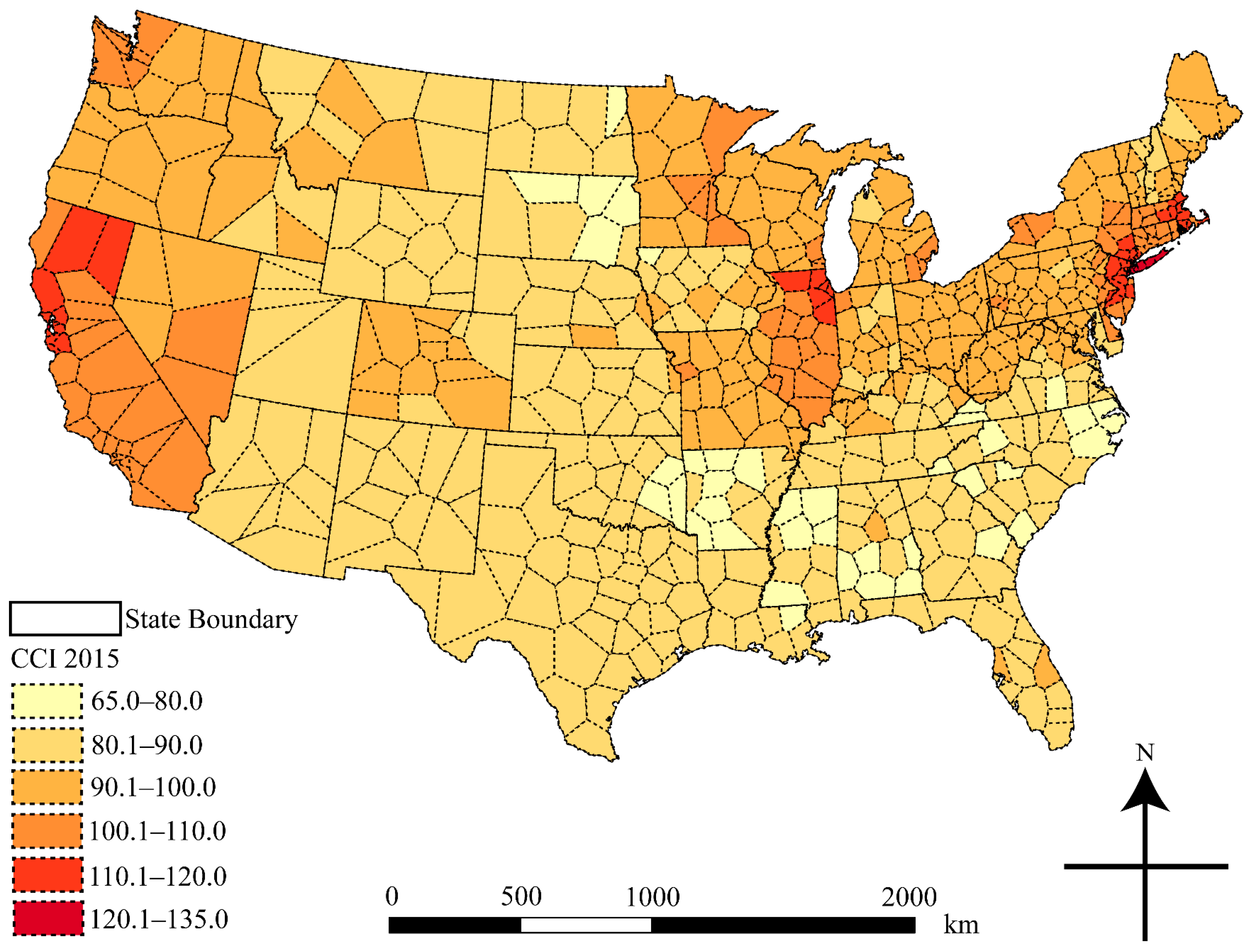
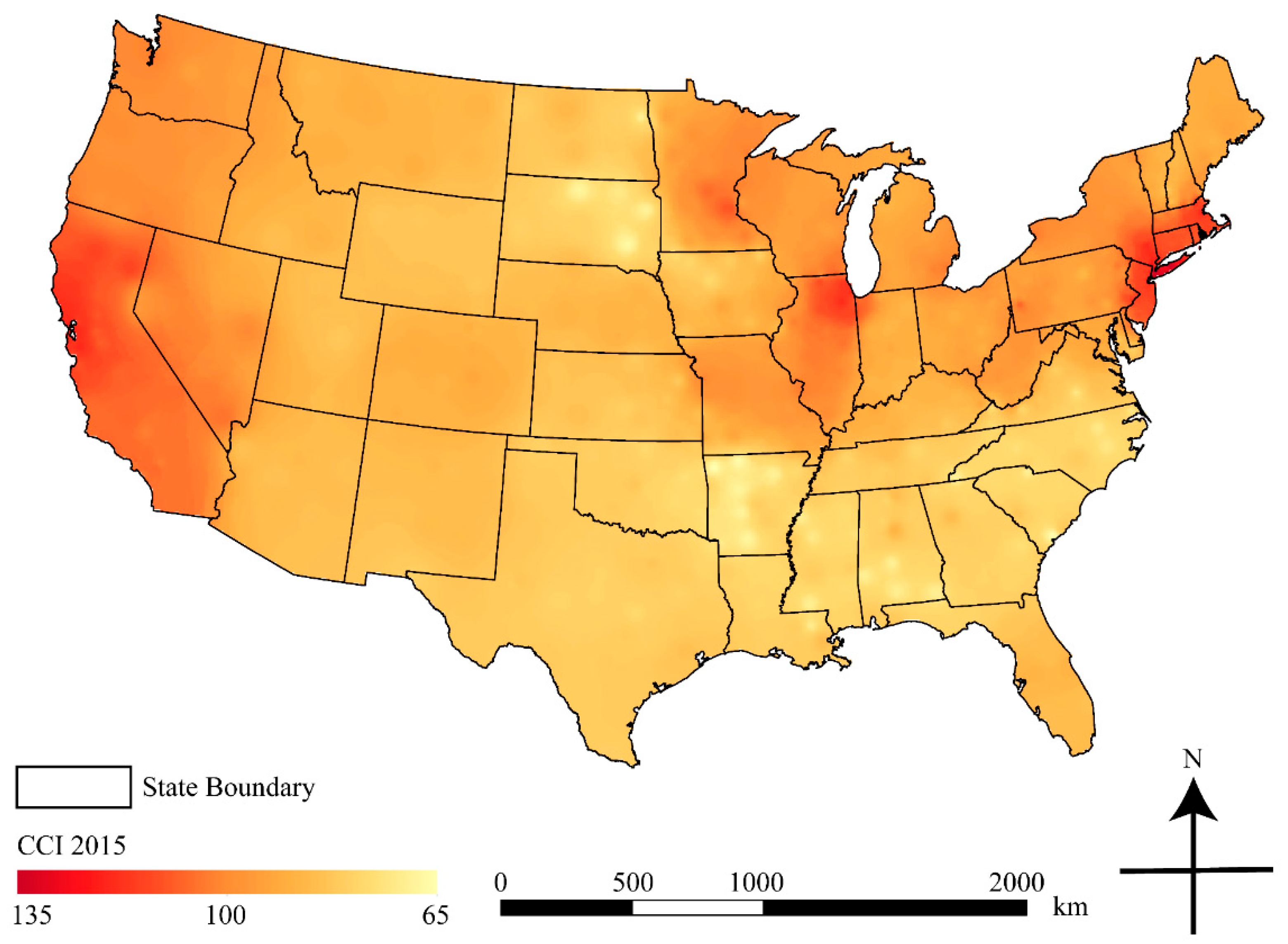
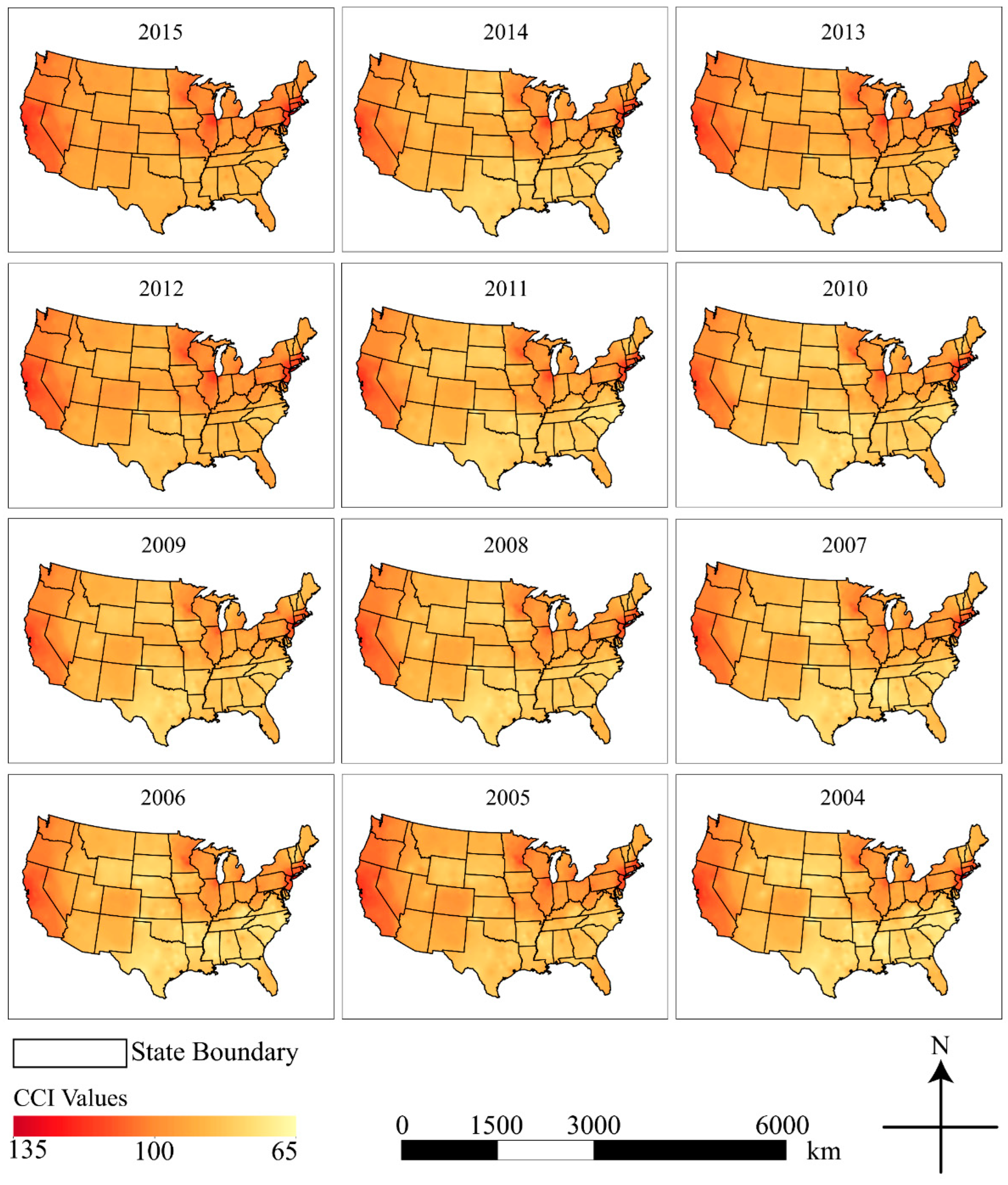
2.4. Mapping Construction Cost

As mentioned in Section 2.2, the IDW interpolation method was selected as the most effective technique for interpolating and mapping construction costs at the national level. Figure 5 has been created to exhibit the overall pattern of construction costs from 2004 to 2015 using the IDW method [7,23,24,25,26,27,28,29,30,31,32,33]. All maps were projected into the U.S. Continuous Lambert Conformal Conic coordinate system. As shown in Figure 5, each year’s construction cost is presented as a smooth surface. The continuous surface fills the voids where no construction cost data exist. IDW interpolated surface maps are also produced in the raster format; therefore, they can be overlaid, meaning values from one map can be compared to another to produce cost change maps at the national level. Figure 6 shows the construction cost differences in one year, two years, five years, and ten years to reveal construction cost variations over the years.

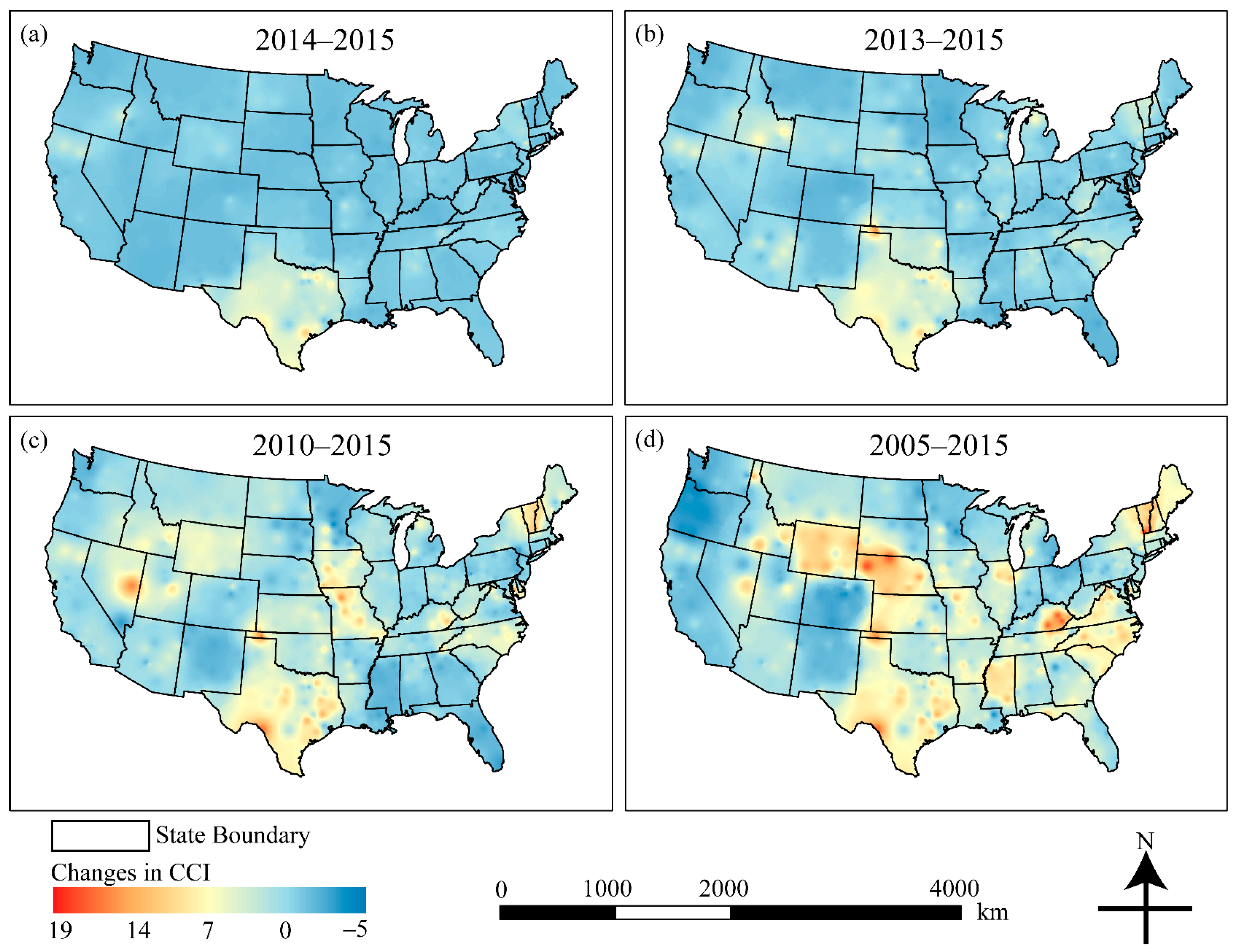
3. Results and Discussion

Currently, construction cost data are released for a limited amount of cities as indexes in a tabular format, which fail to provide a straightforward illustration of national-level construction costs. With the help of the IDW interpolation method, construction cost maps at the national level have been created for multiple years (Figure 5).

Such smooth and continuous surface maps can be used to help construction practitioners, real estate developers, and the public to identify general patterns in the variation of construction costs across the conterminous United States. For example, a general pattern that can be identified from the maps in Figure 5 is that construction costs on the west coast are high, while the construction costs in the central United States are low. The aforementioned users can also identify hot or cold spots correlated with high or low-cost areas for a construction project. For example, construction costs in New York City and Chicago regions are relatively high, while construction costs in the state of Texas are relatively low.

Maps that show the changes in construction costs at the national level over a certain period have also been created for multiple years (Figure 6). It should be noted that the data used in this study are published CCI data from 2004 to 2015. As aforementioned, CCI values are being collected and published on an annual basis by RSMeans. Due to the proprietary nature of RSMeans’ construction cost books, only a fraction of the published CCI data (2004 to 2015) was obtained. However, the data used in this study are irrelevant since this study focuses on demonstrating how to use interpolation methods to create construction cost maps at the national level, including the maps that exhibit changes in construction costs at the national level. The changes in CCI values are represented via increasingly colored hues from cold to warm (e.g., blue to red colors), which are prevalent in exhibiting changes [19]. These cost change maps can be used by investors and businesses to identify economic conditions over time. For example, a one-year construction cost change map (Figure 6a) indicates that construction activity grew remarkably in the state of Texas and in northern California from 2014 to 2015. The ten-year cost change map (Figure 6d) reveals that the states of Wyoming and Nebraska also experienced construction cost growth from 2005 to 2015. On the contrary, the state of Oregon experienced a recession in construction costs during the same period (2005 to 2015).

In a broader context, these maps can also assist with investment forecasting in the real estate industry. For example, a real estate investor might want to compare construction cost maps with home value maps to decide whether investing in existing properties or new construction would be more profitable. For example, cost change maps indicate that northern Ohio experienced a recession in construction costs from 2005 to 2015. If home values remained high, developing new buildings could compete with investment in existing properties. These maps can also provide the public with a quick view of overall economic conditions, which may inform general investment decisions. One future research topic could be exploring the relationship between the construction costs and economic cycles (e.g., recession and economic boom) via relative thematic maps, which hold the potential to provide an alternative and insightful perspective for construction practitioners and academics, real estate developers, investors and businesses, as well as the general public.

One of the robust applications of the national construction cost maps is via web mapping tools to further utilize the capability of geovisualization. Due to the rapid expansion of the internet and the development of web-based geographic information systems (GIS), access to geospatial data on various themes and of varying quality has become significantly easier [34]. When coupled with WebGIS technologies, national construction cost maps can be available to everyone, making accessible the construction cost knowledge that has been traditionally stored in paper-based books or publications. In addition, users can decide which method (NN, CNN, or IDW) to use when visualizing CCI values at the national level. Additionally, the visibility and color schemes of the layers on a web map application can be controlled by the users [35]. That said, the users can decide which method to use, which layers to present, and which color schemes and textures to use, allowing for interactive and dynamic visualization. These WebGIS technologies include not only commercial software programs but also free and open-source software programs, which provide flexibility for different users [36]. Lastly, recent advances in geovisualization provide new methods to visualize geospatial data in a three-dimensional (3D) environment [37]. Visualizing construction costs in a 3D environment holds the potential to identify many patterns that have been impossible in a traditional 2D environment.

Although this research used the CCI as an example of construction costs for mapping, other costs related to construction or costs that contribute to the CCI, such as equipment, material, or labor costs can also be interpolated and mapped at the national level. Construction cost indexes from other suppliers such as the Engineering News-Record (ENR) or highway construction cost index (HCCI) could also be interpolated and mapped at the national level. This research also revealed that interpolation methods can be applied to the geovisualization field to generate cost maps at a large scale.

4. Conclusions

This study investigated the potential of various interpolation methods to visualize construction costs at the national level. The results reveal that maps can provide an effective representation of data where individual values were traditionally represented in a matrix or table of construction costs. The results reveal that a map with a continuous surface provides a better representation of construction costs for cities not listed in the CCI database, and can be readily employed by agencies to visualize their construction cost indexes at the national level. Since construction costs are an indicator of economic conditions, construction cost maps can assist construction and real estate stakeholders, as well as the public, with adjusting their perspectives on economic growth and profitability. Although this research used the CCI as an example of construction costs for mapping, other costs related to construction, such as material or labor costs can also be interpolated and mapped at the national level. Although only a fraction of the published CCI values (i.e., 2004–2015) are used in this study to show the changes in construction costs at the national level, the geovisualization methods used in this study could be easily extended when the additional CCI data (e.g., prior to 2004 and after 2015) are available to reveal patterns over relatively longer temporal periods (e.g., a few decades). The overall contribution of this study to the body of knowledge is the introduction of interpolated maps in visualizing any construction cost-related indexes at a large scale.

References

1. Dlamini, S. Relationship of Construction Sector to Economic Growth. In Working Paper; School of Construction Management and Engineering, University of Reading: Reading, UK, 2016; Available online: http://sitsabo.co.za/docs/misc/cib_paper2012.pdf (accessed on 5 April 2016).
2. Gould, P.E.; Joyce, N. Construction Project Management, 4th ed.; Prentice Hall: Columbus, OH, USA, 2014. [Google Scholar]
3. Sears, S.K.; Sears, G.A.; Clough, R.H.; Rounds, J.L.; Segner, R.O., Jr. Construction Project Management—A Practical Guide to Field Construction Management, 6th ed.; Wiley: New York, NY, USA, 2016. [Google Scholar]
4. U.S. Bureau of Labor Statistics. The Employment Situation—November 2016. In News Release; U.S. Bureau of Labor Statistics: Washington, DC, USA, 2016. [Google Scholar]
5. Dell’Isola, M.D. Architect’s Essentials of Cost Management; John Wiley & Sons, Inc.: New York, NY, USA, 2002. [Google Scholar]
6. Lowe, D.J.; Emsley, M.W.; Harding, A. Predicting Construction Cost Using Multiple Regression Techniques. J. Constr. Eng. Manag. 2006, 132, 750–758. [Google Scholar] [CrossRef] [Green Version]
7. Waier, P.R. Building Construction Cost Data 2014; Robert S. Means Co.: Norwell, MA, USA, 2013. [Google Scholar]
8. Zhang, S.; Bogus, S.M.; Lippitt, C.D.; Migliaccio, G.C. Estimating Location-adjustment Factors for Conceptual Cost Estimating Based on Nighttime Satellite Imagery. J. Constr. Eng. Manag. 2017, 143, 04016087. [Google Scholar] [CrossRef]
9. Dransch, D.; Rotzoll, H.; Poser, K. The Contribution of Maps to the Challenges of Risk Communication to the Public. Int. J. Digit. Earth. 2010, 3, 292–311. [Google Scholar] [CrossRef]
10. Vexler, A.; Hutson, A.D.; Chen, X. Statistical Testing Strategies in the Health Science; CRC Press: Boca Raton, FL, USA, 2016. [Google Scholar]
11. MacEachren, A.M.; Kraak, M. Research Challenges in Geovisualization. Cartogr. Geogr. Inf. Sci. 2001, 28, 3–12. [Google Scholar] [CrossRef]
12. Jiang, B.; Li, Z. Geovisualization: Design, Enhanced Visual Tools and Application. Cartogr. J. 2005, 42, 3–4. [Google Scholar] [CrossRef] [Green Version]
13. Craglia, M.; Shanley, L. Data Democracy—Increased Supply of Geospatial Information and Expanded Participatory Processes in the Production of Data. Int. J. Digit. Earth 2015, 8, 679–693. [Google Scholar] [CrossRef] [Green Version]
14. MacEachren, A.M.; Gahegan, M.; Pike, W.; Brewer, I.; Cai, G.; Lengerich, E.; Hardistry, F. Geovisualization for Knowledge Construction and Decision Support. IEEE Comput. Graph. 2004, 24, 13–17. [Google Scholar] [CrossRef] [PubMed] [Green Version]
15. Migliaccio, G.C.; Zandbergen, P.A.; Martinez, A.A. Empirical Comparison of Methods for Estimating Location Cost Adjustment Factors. J. Manag. Eng. 2013, 31, 04014037. [Google Scholar] [CrossRef]
16. Zhang, S.; Migliaccio, G.C.; Zandbergen, P.A.; Guindani, M. Empirical Assessment of Geographically Based Surface Interpolation for Adjusting Construction Cost Estimates by Project Location. J. Constr. Eng. Manag. 2014, 140, 04014015. [Google Scholar] [CrossRef]
17. Busygin, S.; Prokopyev, O.; Pardalos, P.M. Biculstering in Data Mining. J. Comput. Oper. Res. 2008, 35, 2964–2987. [Google Scholar] [CrossRef]
18. ESRI Data & Maps. Available online: https://www.esri.com/arcgis-blog/products/product/mapping/esri-data-maps/ (accessed on 5 April 2016).
19. MacEachren, A.M.; Taylor, D.R.F. Visualization in Modern Cartography; Elsevier Science: Tarrytown, NY, USA, 1994. [Google Scholar]
20. Bolstad, P. GIS Fundamentals, a First Text on Geographic Information Systems, 2nd ed.; Eider Press: White Bear Lake, MN, USA, 2005. [Google Scholar]
21. Lu, G.; Wong, D. An Adaptive Inverse-Distance Weighting Spatial Interpolation Technique. J. Comput. Geosci. 2008, 34, 1044–1055. [Google Scholar] [CrossRef]
22. Rase, W. Visualization of Polygon-Based Data as a Continuous Surface; Federal Office for Building and Regional Planning: Bonn, Germany, 2009; Available online: http://www.wdrase.de/VisualPycnoInterEngl.pdf (accessed on 16 April 2016).
23. Chiang, J.H.; Plotner, S.C. Building Construction Cost Data 2004; Robert S. Means Co.: Norwell, MA, USA, 2003. [Google Scholar]
24. Balboni, B.; Bastoni, R.A. Building Construction Cost Data 2005; Robert S. Means Co.: Norwell, MA, USA, 2004. [Google Scholar]
25. Waier, P.R. Building Construction Cost Data 2006; Robert S. Means Co.: Norwell, MA, USA, 2005. [Google Scholar]
26. Waier, P.R. Building Construction Cost Data 2007; Robert S. Means Co.: Norwell, MA, USA, 2006. [Google Scholar]
27. Waier, P.R. Building Construction Cost Data 2008; Robert S. Means Co.: Norwell, MA, USA, 2007. [Google Scholar]
28. Waier, P.R. Building Construction Cost Data 2009; Robert S. Means Co.: Norwell, MA, USA, 2008. [Google Scholar]
29. Waier, P.R.; Babbitt, C.; Baker, T.; Balboni, B.; Bastoni, R.A. Building Construction Cost Data 2010; Robert S. Means Co.: Norwell, MA, USA, 2009. [Google Scholar]
30. Waier, P.R.; Babbitt, C.; Baker, T. Building Construction Cost Data 2011; Robert S. Means Co.: Norwell, MA, USA, 2010. [Google Scholar]
31. Waier, P.R.; Charest, A.C.; Babbitt, C.; Baker, T.; Balboni, T. Building Construction Cost Data 2012; Robert S. Means Co.: Norwell, MA, USA, 2011. [Google Scholar]
32. Waier, P.R.; Charest, A.C. Building Construction Cost Data 2013; Robert S. Means Co.: Norwell, MA, USA, 2012. [Google Scholar]
33. Waier, P.R. Building Construction Cost Data 2015; Robert S. Means Co.: Norwell, MA, USA, 2014. [Google Scholar]
34. Kiss, E.; Zichar, M.; Fazekas, I.; Karancsi, G.; Balla, D. Categorization and Geovisualization of Climate Change Strategies Using an Open-Access WebGIS Tool. Infocommun. J. 2020, 12, 32–37. [Google Scholar] [CrossRef]
35. Hoarau, C.; Christophe, S. Cartographic Continuum Rendering Based on Color and Texture Interpolation to Enhance Photo-Realism Perception. ISPRS J. Photogramm. Remote Sens. 2017, 127, 27–38. [Google Scholar] [CrossRef]
36. Balla, D.; Zichar, M.; Toth, R.; Kiss, E.; Karancsi, G.; Mester, T. Geovisualization Techniques of Spatial Environmental Data Using Different Visualization Tools. Appl. Sci. 2020, 10, 6701. [Google Scholar] [CrossRef]
37. Hildebrandt, D. A Software Reference Architecture for Service-Oriented 3D Geovisualization Systems. ISPRS Int. J. Geo-Inf. 2014, 3, 1445–1490. [Google Scholar] [CrossRef] [Green Version]
Figure 1. The 649 CCI cities in the conterminous U.S. and their CCI (city cost index) values in 2015.
Geographies 02 00009 g001
Figure 2. A 2015 construction cost map at the national level created by using the NN (nearest neighbor) method.
Geographies 02 00009 g002
Figure 3. Construction cost map at the national level created by using the CNN (conditional nearest neighbor) method.
Geographies 02 00009 g003
Figure 4. Construction cost map at the national level created by using the IDW (inverse distance weighted) method.
Geographies 02 00009 g004
Figure 5. Multiple construction cost maps at the national level created using the IDW interpolation method.
Geographies 02 00009 g005
Figure 6. Multiple construction cost maps at the national level showing construction cost difference; (a) indicates construction cost difference in one year (2015 value minus 2014 value); (b) indicates construction cost difference in two years (2015 value minus 2013 value); (c) indicates construction cost difference in five years (2015 value minus 2010 value); (d) indicates construction cost difference in ten years (2015 value minus 2005 value).
Geographies 02 00009 g006