Defining Collision Risk: Lesser Flamingo Phoeniconaias minor Power Line Collision Sensitivity and Exposure for Proactive Mitigation

Simple Summary

Determining avian power line collision risk is complicated by numerous factors that influence how, when, and where birds collide with electrical infrastructures. These factors relate to power line collision sensitivity and exposure; however, models describing collision risk often do not address exposure adequately. We explored the importance of power line collision exposure by investigating how it contributed to power line collision risk models for Lesser Flamingos Phoeniconaias minor in South Africa. Our best models suggested that, for Lesser Flamingos, flight height (exposure) and habitat suitability (exposure) were important predictors of collision risk; however, regular nocturnal flights (sensitivity) indicate a need for wire markers that account for nocturnal behavior.

Abstract

Lesser Flamingos Phoeniconaias minor regularly collide with power lines in South Africa. Attaching light-emitting markers to overhead wires seems to be an effective mitigation measure; however, the cost of these devices is prohibitive of large-scale installation. Spatial predictions about flamingo collision risk are thus important for achieving efficient and effective proactive mitigation. In this study, collision risk was defined as a combination of factors related to threat exposure. A habitat suitability index was developed according to changes in surface water occurrence and Chlorophyll-a concentrations, which proved accurate in predicting Lesser Flamingo occurrence. Habitat suitability, and three other species and threat exposure variables, were then used in logistic regression models predicting the occurrence of historic collisions. The most parsimonious model included habitat suitability and flight height. Flamingos were only at risk of collision with power lines when flying lower than 50 m and within 3 km from the water’s edge. High-risk power line sections were thus identified from 3 km buffers around waterbodies ranked according to habitat suitability, which significantly reduced the number of power line spans predicted for proactive marking. While our models indicated that aspects related to exposure were important for predicting flamingo power line collisions, aspects related to sensitivity (e.g., nocturnal behavior) must also guide the choice of mitigation.

1. Introduction

A rising human population and concomitant higher demand for electricity is increasing the exposure of wildlife to the threat of power lines worldwide [1,2]. Avian interactions with power lines result in significant mortalities across distribution and transmission grids. Due to the scale of the problem, these interactions cannot be wholly recorded. Models related to the risk of avian mortalities on power infrastructures (e.g., [3,4]) are thus necessary to predict the spatial distribution of impacts for selected species of conservation concern. There has been a call [4,5,6] for utilities to make a paradigm shift in their approach to dealing with avian collisions with power lines, from reactive to proactive mitigation [7]. A challenge to adopting a proactive mitigation strategy is to obtain a sufficient understanding about the sensitivity of target species (why, how, and to what extent they are affected), as only then can informed predictions be made about future exposure to the risk of power line collisions (where and when they could be affected).

The origin of risk assessment stretches back more than two millennia, being introduced as a decision-making tool by the Athenians [8]. It builds on the premise that risk implies the presence of a certain degree of uncertainty, and, as such, the decision-making process must inherently rely on a mix of qualitative and quantitative data, linking experience and facts [9]. The engineering approach to risk assessment is defined as probability x consequence, hence, an increase in either results in an increase in risk [10]. Two other risk assessment approaches are widely recognized: the actuarial approach and the ecotoxilogical approach [10]. Holton [11] (p. 22) gives a general definition of risk as “…exposure to a proposition of which one is uncertain” and notes further that there cannot be risk without both exposure and uncertainty.

Extinction theory provides a framework for defining the level of risk that certain threats hold for species survival on a global scale, whereby extinction risk is a combination of intrinsic and extrinsic factors. The relationship between different intrinsic and extrinsic factors is often poorly understood because of complicated interactions, and thus identifying potential drivers may be spurious [12]. When modeling the risk of a specific threat to a species, extrinsic and intrinsic risk factors are referred to as exposure and sensitivity, respectively [13]. These terms are commonly applied to the field of ecotoxicology, where sensitivity and exposure measurements form critical steps in the ecological risk assessment paradigm [14]. However, studies from other fields of conservation research rarely model sensitivity and exposure together [15,16], and thus risk may be inadequately described. Single-species risk models usually deal only with factors related to exposure, as sensitivity is mostly assumed to be uniform for all members of a species.

Studies modeling the risk of avian collisions with other electrical infrastructures such as wind turbines (e.g., [17,18,19]) are more frequently reported than those for power lines. This is likely because of a difference in the spatial organization of power line towers and wind turbines; models for linear infrastructures are more complex than radially aggregated ones. For power lines, modeling procedures include a variety of strategies to identify and classify collision risk, but are generally based on estimates of sensitivity, exposure, or a combination of both.

Sensitivity to anthropogenic threats can vary between species. These differences are usually intrinsic, with species being susceptible to a threat based on their ability to sustain, avoid, or adapt to different levels of exposure [20]. For birds, sensitivity with respect to collisions with man-made structures is largely dependent on morphological factors related to vision constraints, e.g., limited binocular visual fields [21], as well as flight, e.g., wing-loading, and low-aspect flight resulting in poor maneuverability and avoidance capability [22,23]. These characteristics are well-represented in the Gruiformes (cranes, bustards, and allies); previous studies have found them to incur high power line collision mortality rates [6,24] compared to other groups. In South Africa, Gruiformes incur a significantly higher proportion of collision mortalities compared to electrocutions.

Exposure refers to the intensity of a threat acting against a species [13,25]. With respect to avian collisions with power lines, it is not practically possible to obtain observations of exposure levels over space and time throughout an entire study area. Conservation practitioners and utilities must therefore rely on models derived from estimates of the probability of exposure. An important, but often ignored, aspect of exposure probability is flight height (although, see [26,27]). It stands to reason that a power line cable only poses a threat if the bird is flying at a collision risk height; thus, the probability of exposure is high if flight height is at, or close to, cable height. The most practical way of obtaining flight height data is to fit GPS and satellite telemetry loggers with altitude sensors to wild birds. Despite recent improvements in the accuracy of these altitude sensors, very few power line collision risk models have incorporated flight height data (however, see [4]). Flight heights have previously been recorded via direct observation (e.g., [28]), although this method has limitations when studying wide-ranging species. Studies making use of this approach typically correlate flight height to terrain or other habitat features to facilitate spatial predictions of potential exposure (e.g., [29]). A caveat to this approach is that models are limited by the spatial input data available. Interactions between different input variables are also not always adequately investigated. For example, in addition to habitat suitability and flight height, the abundance of the animal in question is an important contributor to exposure; and the interaction between these factors may be a more significant predictor than when the variables are considered separately.

The main aim of this study was to develop a theoretical framework for avian power line collision risk modeling in South Africa. To demonstrate this framework, we wished to identify those facets of exposure most likely to predict flamingo collisions with power lines in South Africa.

2. Materials and Methods

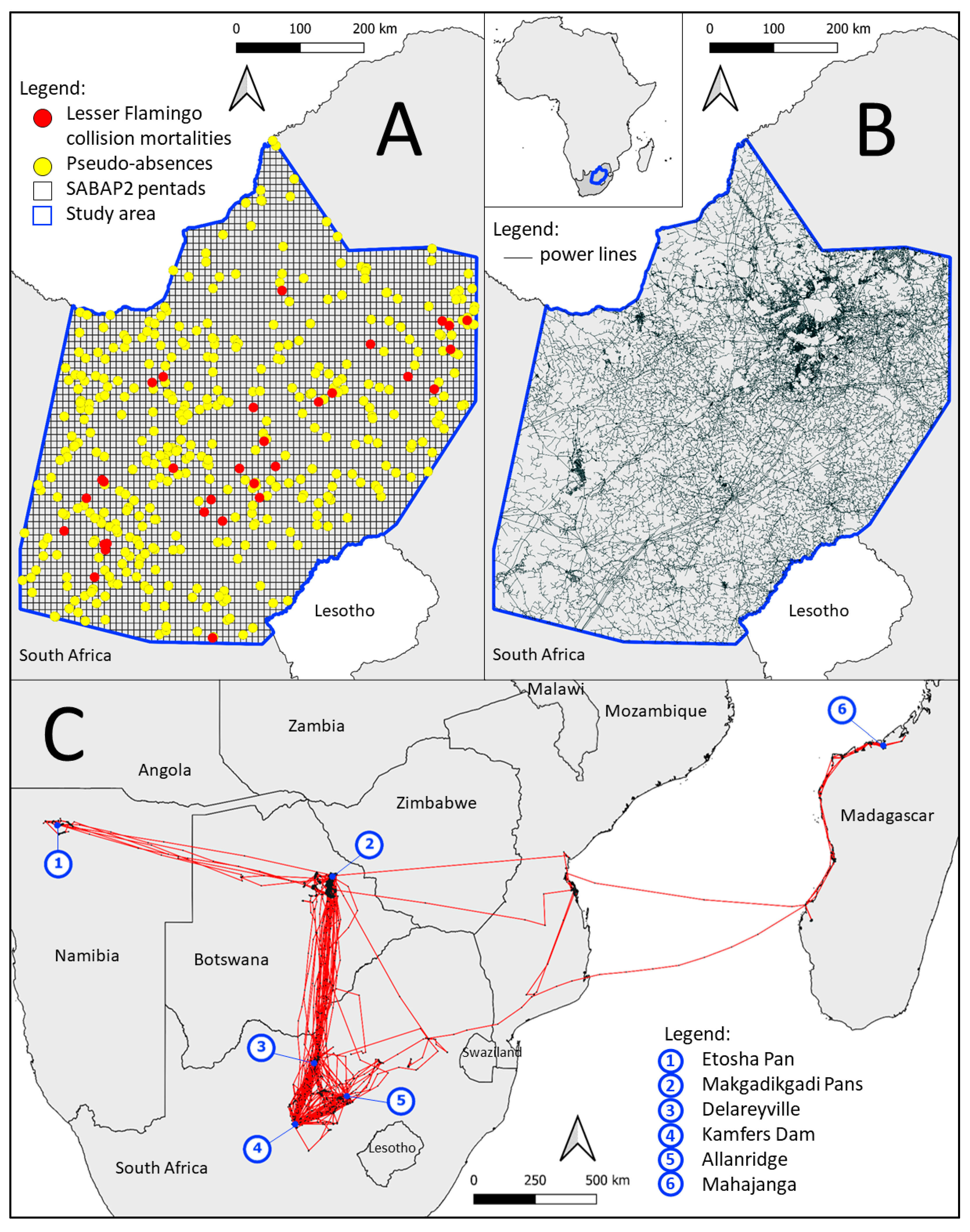
2.1. Study Area

The study area was located in central South Africa and included important breeding and feeding sites within the inland distribution of the Lesser Flamingo [30]. The boundaries of the study area were defined by a 100% minimum convex polygon derived from relocations recorded by 12 GPS-tagged Lesser Flamingos, from March 2016 to November 2018 (Figure 1A). Training and test data used to build the models were taken from power lines (Eskom Holdings Soc. Ltd., Johannesburg, South Africa - hereafter Eskom) restricted to this area, including 13,648 km and 123,081 km of transmission and distribution lines, respectively (Figure 1B). In South Africa, Eskom distribution lines range from 3.3 kV to 132 kV, with power pole heights from 7.5 m to 35 m. Transmission lines range between 132 kV and 765 kV. Transmission line towers include various designs, with tower heights between 25 m and 50 m. Municipal, railway, and other power lines not owned and operated by Eskom, South Africa’s principal power utility, were not considered for this analysis as these data were not available. The area covered all of Gauteng, most of the Free State and North West provinces, and large parts of Limpopo, Mpumalanga, and the Northern Cape provinces of South Africa. It included the most productive parts of the country’s agriculture and mining industries, radiating out from the Witwatersrand, the economic heart of the country, which includes the cities of Johannesburg and Pretoria. Much of the area is thus transformed, and many of the pans and other waterbodies supporting flamingos are surrounded by human settlements. GPS-tagged flamingos were captured at two sites, a salt pan at the Henk Joubert Nature Reserve near Delareyville (26°42′10′′ S, 25°27′21′′ E), North West Province, and a pan near the town of Allanridge (27°46′8′′ S, 26°38′49′′ E) in the Free State Province.

2.2. Data Collection

Trapping and tagging Lesser Flamingos followed methods employed by Childress et al. [31,32]. GPS-GSM satellite transmitters (‘duck’ model, ECOTONE Telemetry, Gdynia, Poland) were attached to the birds by means of Teflon backpack harnesses. Tagging and telemetry methods are described in detail in Pretorius et al. [33]. Devices were set to a GPS fix interval of one fix every 2 h, thus recording a maximum of 12 fixes a day. All GPS fix data were projected to the appropriate UTM coordinate reference system using the spTransform function of the package ‘rgdal’, version 1.4-6, in R [34].

Variables included in Lesser Flamingo collision risk models were considered in a conceptual framework (Appendix A). We assumed that aspects of species sensitivity did not vary among individuals in the population. Nocturnal flight behavior, flight dynamics, and vision are, however, important in determining effective marker types [23]. Lesser Flamingo collision risk exposure variables are discussed below under three categories, namely: habitat suitability, species exposure, and threat exposure.

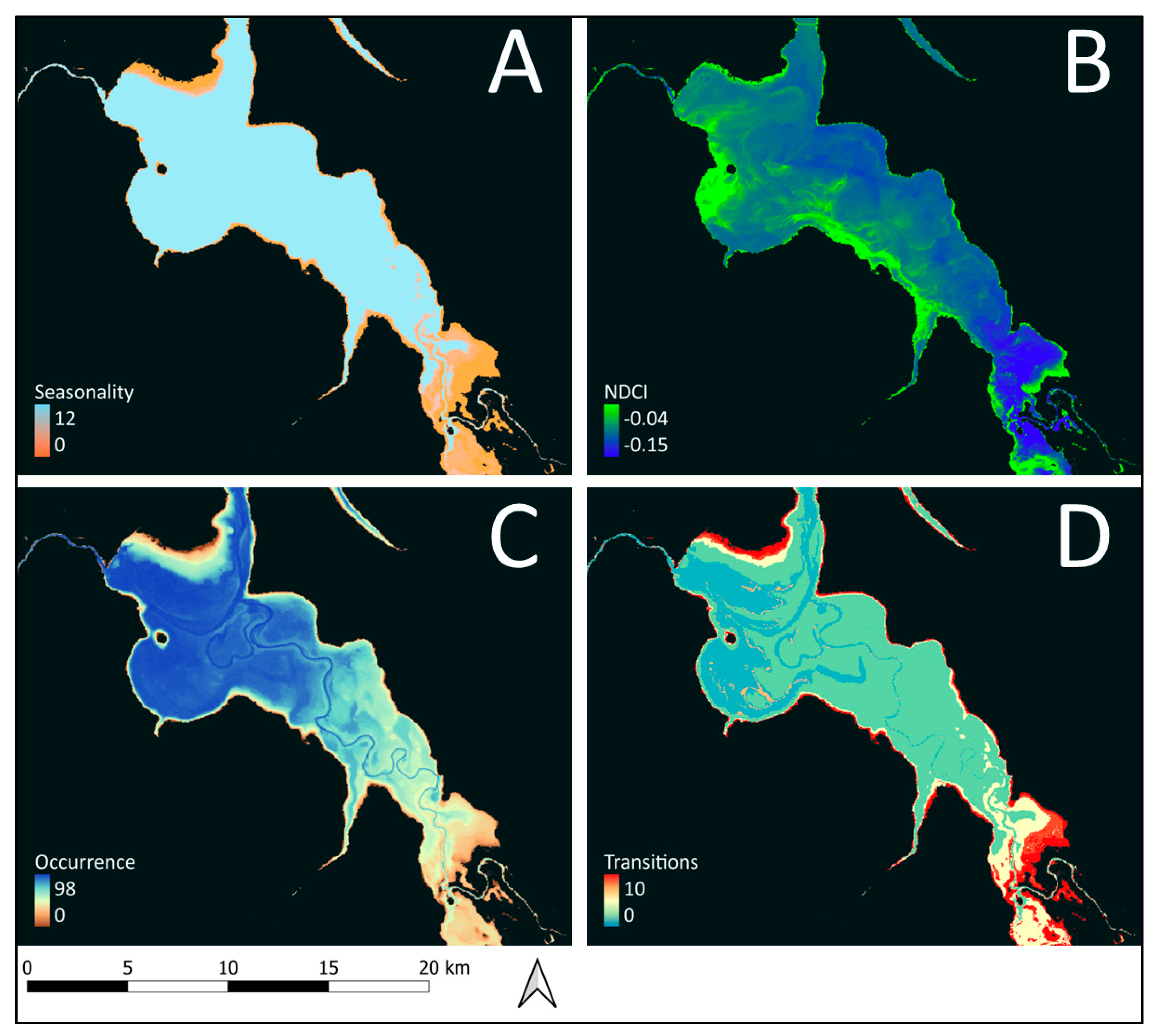
2.2.1. Habitat Suitability Variables

Kellner et al. [35] (p. 476) defines habitat suitability as “…the ability of a habitat to support a viable population over an ecological timescale”. Practically, habitat suitability is the combined interactions between species–habitat relationships, culminating in a value between 0 (completely unsuitable) and 1 (optimal habitat), known as a habitat suitability index (HSI) [36]. Based on previous studies on the ecohydrology of East African lakes and how it relates to Lesser Flamingos [37,38], a habitat suitability index was constructed that reflected both food availability and water quality. Lesser Flamingos feed primarily on filamentous cyanobacteria, mainly Anthrospira sp., and benthic diatoms [39]. The abundance and distribution of these food items can be determined via remote sensing, mapping Chlorophyll-a concentrations at waterbodies occupied by flamingos [38,40].

In order to model food availability for Lesser Flamingos, we prepared a Chlorophyll-a index from the normalized difference chlorophyll index (NDCI) [40]. Landsat images were obtained from the US Geological Survey’s EarthExplorer website https://earthexplorer.usgs.gov/ (accessed 4 December 2018) for 11 scenes covering the study area between March 2016 and November 2018. One cloud-free image was used for each summer and winter period, between the summer of 2016/2017 and winter of 2018. The final dataset thus included 22 images (see Appendix B for Landsat scenes). All of the downloaded images were of the Level 1 GeoTIFF Data Product from the Landsat 8 OLI_TRS sensor. When applied to the Landsat sensor, NDCI is analogous to the normalized difference vegetation index (NDVI) equation [36], thus NDCI = (NIR − red)/(NIR + red), where NIR and red refer to the near-infrared and red bands, respectively. When applied to Landsat 8, the algorithm uses bands 5 (NIR) and 4 (red): NDVI/NDCI = (B5 − B4)/(B5 + B4).

Variables related to water availability and exposure were taken from raster layers prepared for the Global Surface Water Explorer dataset [41], which included 32 years’ data on the extent and change in water surfaces across the globe [42]. The dataset was constructed from layers related to water availability, which included water recurrence (the degree of inter-annual variability in the presence of water), water seasonality (the number of months that water was present in a calendar year), and water transitions (the change in seasonality between the first and last years of the dataset). Variables related to water occurrence included surface water occurrence, ‘SWO’ (the frequency with which water was present on the surface), and occurrence change intensity, ‘∆SWO’ (the change in water occurrence intensity between two epochs). ‘Area’ was taken to be the size of waterbodies, in ha, at maximum surface water occurrence.

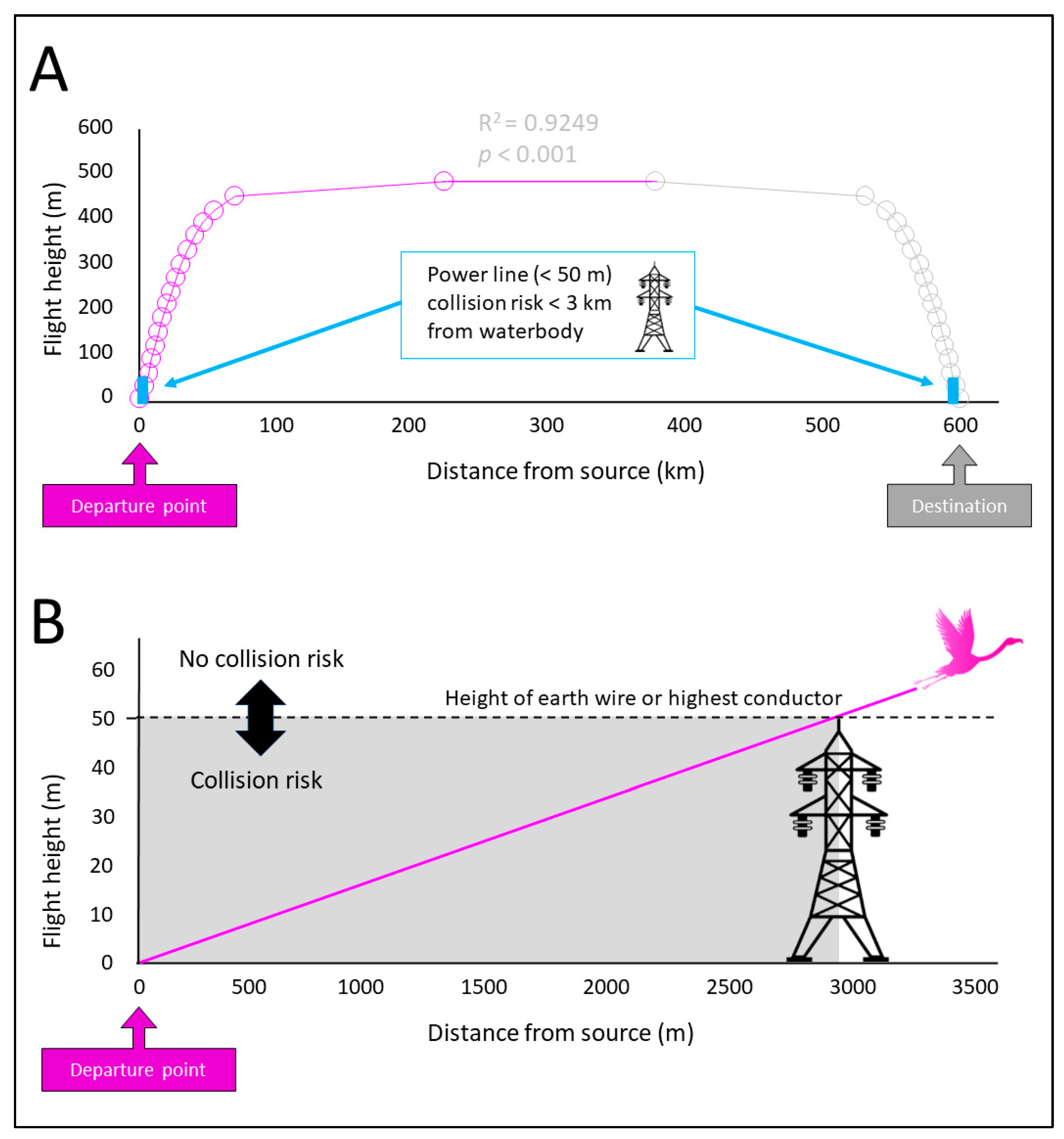
2.2.2. Species Exposure Variables

Flight height was taken from flamingo GPS telemetry data and was expressed in meters above ground level. Correlations between flight height and distance to destination and source during inter-waterbody flights were explored, using a sample of 1138 fixes from six of the GPS-tagged flamingos for which altitude readings were recorded. This enabled mapping of spatially explicit variables indicative of the height that Lesser Flamingos are likely to fly.

The relative density of flamingos at different sites was also assumed to influence exposure, as a greater number of individuals per unit area would increase the probability of contact with a power line cable compared to areas with a lower density of birds. Because counting flamingos across the full extent of the study area was impossible, reporting rates were used as a surrogate for density. Reporting rates were derived from the South African Bird Atlas Project, a citizen-science project aimed at mapping the distribution of all southern African bird species. Previous studies [43,44] show that reporting rates can reliably predict species abundance, given an adequate coverage of surveys throughout the study area.

2.2.3. Threat Exposure Variables

Two threat exposure variables were considered in addition to species exposure and habitat suitability variables, namely, cable height and distance to waterbody. Cable height was taken to be the height of the conductor or earth wire cable of the most common type of tower for a given voltage and was expressed as meters above ground level. Distribution lines typically do not include earth wires, and so power pole heights were considered a proxy for maximum conductor cable height and flamingo collision risk. Most transmission lines have bundled conductors, and only the earth wires are marked. The earth wires are attached to the tops of the towers; thus, the maximum collision risk height for flamingos was taken to be the maximum tower height for each voltage. Distance to waterbody was the distance, in meters, of a power line span to the nearest waterbody edge, as derived from the surface SWO raster layer and a shapefile of Eskom power lines.

2.3. Data Analysis

2.3.1. Habitat Suitability Index

Logistic regression was used in two different models: (1) an analysis of Lesser Flamingo habitat suitability and (2) a predictive model of Lesser Flamingo collision mortality. Because the nature of the response variable is binary in logistic regression, habitat suitability was predicted based on waterbodies visited (coded 1) against those not visited (coded 0) by Lesser Flamingos. These data were obtained from GPS telemetry relocations, with waterbodies not visited taken to be those bisected by Lesser Flamingo flightpaths without the birds landing (<5 m flight height) and stopping (<1 relocation) at the waterbody. Several a priori multivariate logistic regression models were constructed from combinations of predictor variables described above: NDCI, waterbody area, SWO, ∆SWO, water recurrence, water seasonality, and water transitions. The number of the independent variables included in the models were reduced in two steps: Collinearity between variables was investigated by means of a correlation matrix of Spearman’s correlations between variables using the package ‘PerformanceAnalytics’, version 1.5.2, in R [45]. Predictor variables that resulted in a poor fit to the logistic response were omitted from the final set of models by means of a backward stepwise elimination process in R, using the ‘stepAIC’ function in the package ‘MASS’, version 7.3-51.1 [46]. Once the most parsimonious model was determined using the above procedure, a habitat suitability index was created for each of the waterbodies within the study area using the model formula and the raster calculator in Quantum GIS (QGIS).

2.3.2. Collision Risk Models

The logistic regression model procedures above were repeated in a Lesser Flamingo collision risk model, with the dependent response variable ‘collision’ coded 1 (n = 32) or 0 (n = 384) for power line sections where collision mortalities have or have not been recorded within the study area in the past 22 years (1997–2018). The (0) points used to train the model were considered pseudo-absences selected from power line sections within the study area. The model was built on a ratio of 1:12 presence vs. pseudo-absence points, where the latter were selected based on a conditional random selection, where the distance between presence and pseudo-absence points was ≥1 km, using the Create Random Points tool in QGIS (Data Management toolbox—Sampling toolset). Selection of pseudo-absences was random and unbalanced as this is the preferred method in regression-based techniques for mapping distributions [47]. Collision risk was modeled against four independent variables: habitat suitability, flight height, cable height, and reporting rate. Final models were evaluated according to Akaike weights, based on the small sample correction for Akaike’s Information Criteria (AICc), and ranked using delta AICc (∆AICc) and the package ‘AICcmodavg’ in R [48]. Candidate models were those within 2∆AICc of the top-ranked model [49].

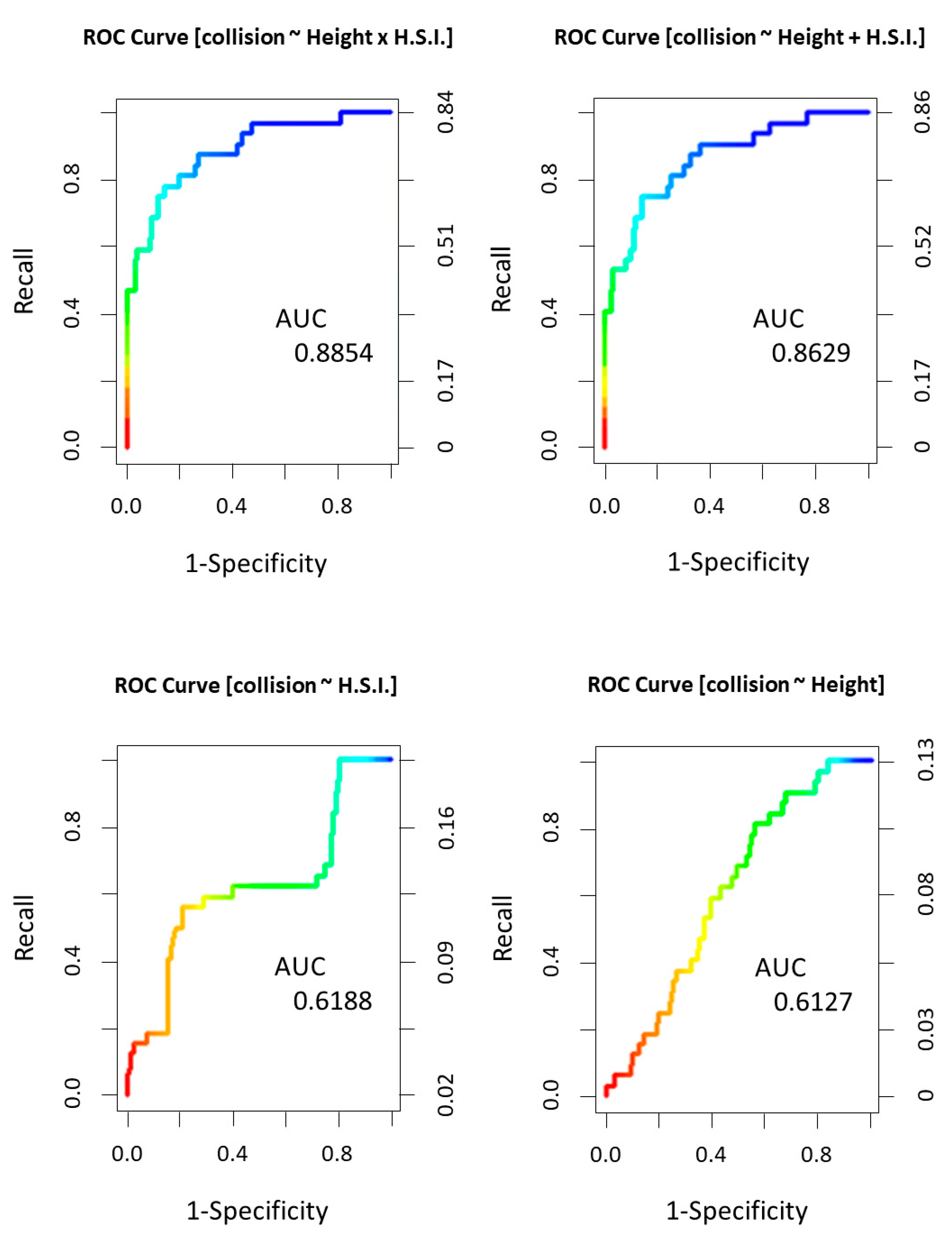
2.3.3. Model Validation

The performance of the most parsimonious habitat suitability model was validated in the field using a sample of 20 waterbodies. Ten of these were classified as high habitat suitability and ten as low habitat suitability according to the habitat suitability index, thus predicting presence and absence, respectively. Predicted, versus real, presences and absences were then used to gauge the model’s accuracy, precision, and area-under-the-curve (AUC) using the ConfusionMatrix function of the package ‘caret’ [50]. For collision risk, candidate models were assessed based on the same statistical procedures in R, except that validation was desktop-based by generating pseudo-absences. An AUC value closer to 1.0 than 0.5 was considered significantly different to what is expected from normal. Models with AUC values falling below 0.5 were considered a poor fit to the training data. Finally, receiver operating characteristic (ROC) curves were plotted to illustrate the ratio between sensitivity and (1-) specificity for candidate models. Statistical significance was α = 0.05 for all tests.

3. Results

3.1. Lesser Flamingo Habitat Suitability

The manipulation of Landsat-8 raster bands using the NDCI algorithm produced images clearly showing chlorophyll concentrations in waterbodies within the study area (Figure 2). For multivariate analyses, all the candidate models included a combination of NDCI and NDCImax, indicating that these indices, when combined, were good predictors of Lesser Flamingo food availability. The model with these two variables alone was, however, not as strong a fit as those including ∆SWO and water recurrence. The most parsimonious model separating waterbodies visited and those not visited by Lesser Flamingos included change in surface water occurrence (∆SWO). Only two of the models evaluated fell within ≤ ∆AICc, and within the 95% confidence set (

Table 1. The top-ranked models describing Lesser Flamingo occupancy as a function of habitat. NDCI = normalized difference chlorophyll index. ∆SWO = change in surface water occurrence. ‘Visited’ is a binary response variable denoting Lesser Flamingo presences (1) and absences (0), as derived from the movements of GPS-tagged individuals. K = number of model parameters, AICc = sample correction for Akaike’s Information Criterion, ∆AICc = delta AIC, w = Akaike weight, cum.w = cumulative w.

Model	K	AICc	∆AICc	w	cum.w
Visited ~ ∆SWO + NDCI + NDCImax	4	213.990	0.000	0.533	0.533
Visited ~ Water recurrence + NDCI + NDCImax	4	214.540	0.540	0.407	0.939
Visited ~ NDCI + NDCImax	3	218.440	4.450	0.058	0.997

).

Entering the model equation into a QGIS raster calculator resulted in a habitat suitability index used in collision risk modeling. Field validation of a binary reclassification of the HSI, where 0 represents waterbodies predicted not to be suitable and 1 those predicted to be suitable for Lesser Flamingos, showed that the habitat suitability index was good at predicting where flamingos occurred (positive predictive value, PPV = 0.92) and where they did not (negative predictive value, NPV = 0.83), with an overall model accuracy of 0.88 (sensitivity = 0.85, specificity = 0.91).

3.2. Species Exposure

The relationship between flight height and distance to source and destination waterbodies was best described by a polynomial curve (Figure 3). The relationship was significant (R² = 0.93, p < 0.001), and suggested that Lesser Flamingos flew higher during the longer, middle sections of their flights, ascending and descending rapidly closer from/to their departure point and destination. This meant that only a small portion of each flight was at a height that exposed flamingos to potential collision mortality, i.e., during a flight between waterbodies, they only flew at a collision risk height (<50 m) within 3 km from the departure point and destination. The formula of the curve was used to create a surrogate variable to denote Height for all data points used to train the final logistic regression models.

The frequency with which Lesser Flamingos were encountered within each SABAP2 pentad containing waterbodies varied considerably ($\overline{\mathrm{x}}$ = 3.64%, variance = 208.90%), from 0% to 100% reporting rate. Reporting rates were significantly higher for pentads from which flamingo collision mortalities were reported, compared to those containing pseudo-absences (Mann–Whitney U = 4018, p < 0.001).

3.3. Multivariate Collision Risk Models

Because the variables flight height and distance to waterbody were correlated, only flight height was retained for the stepwise backwards regression. Only two variables fit the collision response data well: flight height and habitat suitability (

Table 2. Parameter coefficients and probabilities from logistic regression describing Lesser Flamingo collision risk.

Coefficients	Estimate	SE	z Value	p
(Intercept)	−3.923	1.331	−2.947	0.003
Flight height	−0.014	0.005	−2.743	0.006
Habitat suitability	1.763	0.643	2.740	0.006
Reporting rate	0.013	0.009	1.36106	0.173
Cable height	−0.061	0.055	−1.11236	0.266

). These were thus retained for the final set of models. Multivariate models suggested that an interaction term between height and habitat suitability was most likely to provide an accurate prediction of the risk that power line sections hold for Lesser Flamingos (

Table 3. Top-ranked models describing Lesser Flamingo collision risk as a function of power line collision exposure. K = number of model parameters, AICc = sample correction for Akaike’s Information Criterion, ∆AICc = delta AIC, w = Akaike weight, cum.w = cumulative w.

Model	K	AICc	∆AICc	w	cum.w
Collision ~ flight height x habitat suitability	4	209.08	0	0.73	0.73
Collision ~ flight height + habitat suitability	3	211.12	2.04	0.26	1
Collision ~ habitat suitability	2	220.13	11.05	0	1
Collision ~ flight height	2	221.34	12.26	0	1

). This model was also the only one within the 95% confidence set and within ≤2 ∆AICc. Evaluating model performance via the validation methods described above, the model with the flight height x habitat suitability also resulted in a slightly better area-under-the-curve (AUC) statistic and ROC curve (Figure 4) than flight height + habitat suitability.

4. Discussion

In this study, we explored the different components of risk in predicting power line collisions for Lesser Flamingos in South Africa. The single-species approach negated aspects related to sensitivity in the models. In the case of the Lesser Flamingo, they may include aspects such as flight behavior, maneuverability, and vision. Binocular vision and visual acuity of birds as they relate to power line collision mortality has been reviewed [51]. The binocular visual fields of flamingos are narrower, but vertically longer, than some other collision-prone species such as bustards and cranes [52]. Lesser Flamingo collisions tend to be clumped, usually with several mortalities in one incident. Flamingos rank second out of all groups of birds on the Eskom-EWT Partnership’s Central Incident Register in terms of the number of mortalities (individuals) recorded per incident. Apart from restricted visual fields, these events may be related to flight behavior as Lesser Flamingos fly in close-knit flocks and conduct most of their inter-waterbody movements at night [33], a fact that is assumed to affect their collision sensitivity. Aspects of flight behavior may thus be useful for modeling the temporal aspects of collision sensitivity. Additional aspects may also contribute to temporal changes to collision sensitivity; conditions that adversely affect visibility, e.g., mist, fog, or inclement weather, are assumed to increase collision sensitivity [2]. However, Pannucio et al. [53] suggest that migrating birds avoid flying through fog and low clouds. These temporal aspects should be investigated specifically for Lesser Flamingos to improve our interpretation of their collision sensitivity and collision risk models.

A few assumptions have been made in the modeling of collision risk for Lesser Flamingos, and these should be validated for a more realistic representation of some of the parameters used. Regarding habitat suitability, NDCI should be viewed as an index only, as it does not relate to real measurements of Chlorophyll-a; these need to be calibrated to in situ measurements sampled from the waterbodies. Regarding our assumptions about flamingo densities, while SABAP2 reporting rates can be used as a surrogate for species density [43,44], we acknowledge the limitations of using citizen-science data. These authors do, however, show that reporting rates correlate more significantly with density for larger, more conspicuous birds; thus, we believe that our assumption in this regard is realistic.

We have demonstrated that exposure to a threat is not related to some prediction of habitat use or suitability alone, but rather incorporates different aspects related to the species and the threat. In the case of the Lesser Flamingo, the best model predicting collision mortality risk included an interaction between habitat suitability along with a measure of the exposure potential in the form of flight height. Another important consideration is that estimates of habitat suitability cannot be made from data sampled outside of that which is available to an animal. We believe that our sampling regime accounts for this by using GPS-telemetry data to define the study area and the waterbodies considered for the analysis. A challenge for multi-species collision risk models is the availability of telemetry data for all species considered within the same study area; thorough vantage point surveys can provide useful observations about bird flightpaths and flight heights, although these are typically only obtained for specific locations earmarked for energy infrastructure development.

Considering the above, we propose two frameworks for spatial species collision risk modeling. The first involves a single species; thus, aspects of sensitivity need not be incorporated. Collision risk models for single species should be constructed using the following framework:

C = HSI + Exposure_sp + Exposure_threat,

where C is collision risk, HSI is a habitat suitability index, Exposure_sp relates to properties of the species flight characteristics and/or population density, and Exposure_threat involves the spatial distribution, density, and nature of the threat itself (e.g., the height of power lines, inclusion of earth wires, etc.). A second type of collision risk model involves multiple species, which requires the inclusion of aspects related to species sensitivity to collision. The sensitivity of one species is thus relative to the others included in the models. In both cases, estimates of habitat suitability should be determined from points sampled within the area available to the species. In the case of species not restricted to a habitat as specific as the Lesser Flamingo, habitat suitability can be determined from species distribution models. A simple framework for these models is given as:

Ci = Sensitivity x (HSI + Exposuresp + Exposurethreat)

and

C_total = ∑ (C_i)

where C_i is the collision risk for a single species, and C_total is the combined collision risk for all species considered.

The above-mentioned frameworks compliment the models of Gauld et al. [20], who incorporated GPS-tracking data to determine collision sensitivity. They differ from other collision risk models, such as those described by D’Amico et al. [20], who developed indexes based on morphological and behavioral traits as a surrogate for sensitivity.These frameworks could be used to inform the deployment of species-specific mitigation measures. A total of twelve Lesser Flamingo collision mortalities have been recorded on the Eskom/EWT Central Incident Register since our model was developed, nine of which were within the study area. Six of the nine incidents were found under line sections identified as high risk by the model (i.e., power lines within 3 km of high-quality waterbodies); thus, proactive mitigation on high-priority line sections could have prevented these mortalities. A preliminary study suggests that flamingo collisions could be successfully mitigated using markers such as the Nocturnal Overhead Warning Light (‘OWL’) device, a marker with solar-powered light-emitting diodes (LEDs), developed specifically for birds with nocturnal habits [54]. Such devices are expensive and cannot be deployed everywhere, hence the need to predict the location of high-risk areas for prioritizing marking interventions. New energy generation infrastructure developments such as wind energy facilities may also benefit from the information contained within this paper, as flamingos are susceptible to collisions with wind turbines, and determining buffer zones is an important consideration for environmental impact assessments.

References

1. Jenkins, A.R.; Smallie, J.J.; Diamond, M. Avian collisions with power lines: A global review of causes and mitigation with a South African perspective. Bird Conserv. Int. 2010, 20, 263–278. [Google Scholar] [CrossRef]
2. Bernardino, J.; Bevanger, K.; Barrientos, R.; Dwyer, J.F.; Marques, A.T.; Martins, R.C.; Shaw, J.M.; Silva, J.P.; Moreira, F. Bird collisions with power lines: State of the art and priority areas for research. Biol. Conserv. 2018, 222, 1–13. [Google Scholar] [CrossRef]
3. Dwyer, J.F.; Harness, R.E.; Donohue, K. Predictive model of avian electrocution risk on overhead power lines. Conserv. Biol. 2014, 28, 159–168. [Google Scholar] [CrossRef]
4. Silva, J.P.; Palmeirim, J.M.; Alcazar, R.; Correia, R.; Delgado, A.; Moreira, F. A spatially explicit approach to assess the collision risk between birds and overhead power lines: A case study with the little bustard. Biol. Conserv. 2014, 170, 256–263. [Google Scholar] [CrossRef]
5. Heck, N. A Landscape-Scale Model to Predict the Risk of Bird Collisions with Electric Power Transmission Lines in Alberta. Master Thesis, University of Calgary, Alberta, Canada, 2017. [Google Scholar]
6. Shaw, J.M.; Jenkins, A.R.; Smallie, J.J.; Ryan, P.G. Modelling power-line collision risk for the Blue Crane Anthropoides paradiseus in South Africa. Ibis 2010, 152, 590–599. [Google Scholar] [CrossRef]
7. Pretorius, M.D.; Hoogstad, C. An Avian Red-List Sensitivity Map Relevant to Eskom Distribution Power Lines in South Africa; Report no. RES/RR/15/1785097; Eskom Holdings SOC Ltd.: Johannesburg, South Africa, 2016. [Google Scholar]
8. Bernstein, P.L. Against the Gods: The Remarkable Story of Risk; John Wiley and Sons: New York, NY, USA, 1996. [Google Scholar]
9. Hertz, D.B.; Thomas, H. Risk Analysis and its Applications; Wiley: Chichester, UK, 1983. [Google Scholar]
10. Kirkland, L.-H.; Thompson, D. Environmental Management Systems. In Tools for Environmental Management: A Practical Introduction and Guide; Thompson, D., Ed.; New Society Publishers: Gabriola Island, BC, Canada, 2002; pp. 19–42. [Google Scholar]
11. Holton, G.A. Defining risk. Financ. Anal. J. 2004, 60, 19–25. [Google Scholar] [CrossRef]
12. Blackburn, T.M.; Gaston, K.J. Extrinsic factors and the population sizes of threatened birds. Ecol. Lett. 2002, 5, 568–576. [Google Scholar] [CrossRef]
13. Dickinson, M.G.; Orme, C.D.L.; Suttle, K.B.; Mace, G.M. Separating sensitivity from exposure in assessing extinction risk from climate change. Sci. Rep. 2014, 4, 6898. [Google Scholar] [CrossRef] [PubMed]
14. Burger, J. A risk assessment for lead in birds. J. Toxicol. Env. Health 1995, 45, 369–396. [Google Scholar] [CrossRef]
15. Fischer, D.O.; Blomberg, S.P.; Owens, I.P.F. Extrinsic versus intrinsic factors in the decline and extinction of Australian marsupials. Proc. R. Soc. B: Biol. Sci. 2003, 270, 1801–1808. [Google Scholar] [CrossRef]
16. Gauld, J.G.; Silva, J.P.; Atkinson, P.W.; Record, P.; Acácio, M.; Arkumarev, V.; Blas, J.; Bouten, W.; Burton, N.; Catry, I.; et al. Hotspots in the grid: Avian sensitivity and vulnerability to collision risk from energy infrastructure interactions in Europe and North Africa. J. Appl. Ecol. 2022, 59, 1496–1512. [Google Scholar] [CrossRef]
17. Desholm, M.; Kahlert, J. Avian collision risk at an offshore wind farm. Biol. Lett. 2005, 1, 296–298. [Google Scholar] [CrossRef]
18. Chamberlain, D.E.; Rehfisch, M.R.; Fox, A.D.; Desholm, M.; Anthony, S.J. The effect of avoidance rates on bird mortality predictions made by wind turbine collision risk models. Ibis 2006, 148, 198–202. [Google Scholar] [CrossRef]
19. Krijgsveld, K.L.; Akershoek, K.; Schenk, F.; Dijk, F.; Dirksen, S. Collision risk of birds with modern large wind turbines. Ardea 2009, 97, 357–366. [Google Scholar] [CrossRef]
20. D’Amico, M.; Martins, R.C.; Álvarez-Martínez, J.M.; Porto, M.; Barrientos, R.; Moreira, F. Bird collisions with power lines: Prioritizing species and areas by estimating potential population-level impacts. Divers. Distrib. 2019, 25, 975–982. [Google Scholar] [CrossRef]
21. Martin, G.R.; Shaw, J.M. Bird collisions with power lines: Failing to see the way ahead? Biol. Conserv. 2010, 143, 2695–2702. [Google Scholar] [CrossRef]
22. Bevanger, K. Bird interactions with utility structures: Collision and electrocution, causes and mitigation measures. Ibis 1994, 136, 412–425. [Google Scholar] [CrossRef]
23. Janss, G.F.E. Avian mortality from power lines: A morphologic approach of a species-specific mortality. Biol. Conserv. 2000, 95, 353–359. [Google Scholar] [CrossRef]
24. Shaw, J.M.; Reid, T.A.; Gibbons, B.K.; Pretorius, M.D.; Jenkins, A.R.; Visagie, R.; Michael, M.D.; Ryan, P.G. A large-scale experiment demonstrates that line marking reduces power line collision mortality for large terrestrial birds, but not bustards, in the Karoo, South Africa. Condor 2021, 123, duaa067. [Google Scholar] [CrossRef]
25. Purvis, A.; Gittleman, J.L.; Cowlishaw, G.; Mace, G.M. Predicting extinction risk in declining species. Proc. R. Soc. B Biol. Sci. 2000, 267, 1947–1952. [Google Scholar] [CrossRef] [PubMed]
26. Marcelino, J.; Moreira, F.; Franco, A.M.; Soriano-Redondo, A.; Acacio, M.; Gauld, J.; Rego, F.C.; Silva, J.P.; Catry, I. Flight altitudes of a soaring bird suggest landfill sites as power line collision hotspots. J. Environ. Manag. 2021, 294, 113–149. [Google Scholar] [CrossRef]
27. Gustin, M.; Giglio, G.; Pellegrino, S.C.; Frassanito, A.; Ferrarini, A. Nocturnal flights lead to collision risk with power lines and wind farms in Lesser Kestrels: A preliminary assessment through GPS tracking. Comput. Ecol. Softw. 2018, 8, 15–22. [Google Scholar]
28. Rollan, À.; Real, J.; Bosch, R.; Tintó, A.; Hernández-Matías, A. Modelling the risk of collision with power lines in Bonelli’s Eagle Hieraaetus fasciatus and its conservation implications. Bird Conserv. Int. 2010, 20, 279–294. [Google Scholar] [CrossRef]
29. Reid, T.; Kruger, S.; Whitfield, D.P.; Amar, A. Using spatial analyses of bearded vulture movements in southern Africa to inform wind turbine placement. J. Appl. Ecol. 2015, 52, 881–892. [Google Scholar] [CrossRef]
30. Anderson, M.D. Lesser Flamingo Phoeniconaias minor. In The 2015 Eskom Red Data Book of Birds of South Africa, Lesotho and Swaziland; Taylor, M.R., Peacock, F., Wanless, R.M., Eds.; BirdLife South Africa: Johannesburg, South Africa, 2015; pp. 305–307. [Google Scholar]
31. Childress, B.; Harper, D.; Hughes, B.; Van der Bossche, W.; Berthold, P.; Querner, U. Satellite tracking Lesser Flamingo movements in the Rift Valley, East Africa: Pilot study report. Ostrich 2004, 75, 57–65. [Google Scholar] [CrossRef]
32. Childress, B.; Harper, D.; Ferris, C. Sex determination in the Lesser Flamingo (Phoenicopterus minor) using morphological measurements. Ostrich 2005, 76, 148–153. [Google Scholar] [CrossRef]
33. Pretorius, M.D.; Leeuwner, L.; Tate, G.J.; Botha, A.; Michael, M.D.; Durgapersad, K.; Chetty, K. Movement patterns of lesser flamingos Phoeniconaias minor: Nomadism or partial migration? Wildl. Biol. 2020, 2020, wlb.00728. [Google Scholar] [CrossRef]
34. Bivand, R.; Keitt, T.; Rowlingson, B. Rgdal: Bindings for the ‘Geospatial’ Data Abstraction Library. R Package Version 1.4-6. 2019. Available online: https://CRAN.R-project.org/package=rgdal (accessed on 31 January 2020).
35. Kellner, C.J.; Brawn, J.D.; Karr, J.R. What is habitat suitability and how should it be measured? In Wildlife 2001: Populations; McCullough, D.R., Barrett, R.H., Eds.; Elsevier Applied Science: London, UK; New York, NY, USA, 1992; pp. 476–488. [Google Scholar]
36. Verner, J.; Morrison, M.L.; Ralph, C.J. Wildlife 2000: Modeling Habitat Relationships of Terrestrial Vertebrates; University of Wisconsin Press: Madison, WI, USA, 1986. [Google Scholar]
37. Tebbs, E.J.; Remedios, J.J.; Harper, D.M. Remote sensing of chlorophyll-a as a measure of cyanobacterial biomass in Lake Bogoria, a hypertrophic, saline–alkaline, flamingo lake, using Landsat ETM+. Remote Sens. Environ. 2013, 135, 92–106. [Google Scholar] [CrossRef]
38. Tebbs, E.J.; Remedios, J.J.; Avery, S.T.; Harper, D.M. Remote sensing the hydrological variability of Tanzania’s Lake Natron, a vital Lesser Flamingo breeding site under threat. Ecohydrol. Hydrobiol. 2013, 13, 148–158. [Google Scholar] [CrossRef]
39. Krienitz, L.; Krienitz, D.; Dadheech, P.K.; Hübener, T.; Kotut, K.; Luo, W.; Teubner, K.; Versfeld, W.D. Food algae for Lesser Flamingos: A stocktaking. Hydrobiologia 2016, 775, 21. [Google Scholar] [CrossRef]
40. Mishra, S.; Mishra, D.R. Normalized difference Chlorophyll index: A novel model for remote estimation of Chlorophyll-a concentration in turbid productive waters. Remote Sens. Environ. 2012, 117, 394–406. [Google Scholar] [CrossRef]
41. Pekel, J.-F.; Cottam, A.; Gorelick, N.; Belward, A. Global Surface Water Explorer Dataset. European Commission, Joint Research Centre (JRC). 2017. Available online: http://data.europa.eu/89h/jrc-gswe-global-surface-water-explorer-v1 (accessed on 20 February 2019).
42. Pekel, J.-F.; Cottam, A.; Gorelick, N.; Belward, A. High-resolution mapping of global surface water and its long-term changes. Nature 2016, 540, 418–422. [Google Scholar] [CrossRef] [PubMed]
43. Lee, A.T.; Altwegg, R.E.S.; Barnard, P. Estimating conservation metrics from atlas data: The case of southern African endemic birds. Bird Conserv. Int. 2017, 27, 323–336. [Google Scholar] [CrossRef]
44. Lee, A.T.; Fleming, C.; Wright, D.R. Modelling bird atlas reporting rate as a function of density in the southern Karoo, South Africa. Ostrich 2018, 89, 363–372. [Google Scholar] [CrossRef]
45. Peterson, B.G.; Carl, P. Performance Analytics: Econometric Tools for Performance and Risk Analysis. R Package Version 1.5.2. 2018. Available online: https://CRAN.R-project.org/package=PerformanceAnalytics (accessed on 30 November 2018).
46. Venables, W.N.; Ripley, B.D. Modern Applied Statistics with S, 4th ed.; Springer: New York, NY, USA, 2002. [Google Scholar]
47. Barbet-Massin, M.; Jiguet, F.; Albert, C.H.; Thuiller, W. Selecting pseudo-absences for species distribution models: How, where and how many? Methods Ecol. Evol. 2012, 3, 327–338. [Google Scholar] [CrossRef]
48. Mazerolle, M.J. AICcmodavg: Model Selection and Multimodel Inference Based on (Q)AIC(c). R Package Version 2.3-2. 2017. Available online: https://cran.pau.edu.tr/web/packages/AICcmodavg/AICcmodavg.pdf (accessed on 31 January 2020).
49. Burnham, K.P.; Anderson, D.R. Model Selection and Inference: A Practical Information-Theoretic Approach; Springer: New York, NY, USA, 2002. [Google Scholar]
50. Kuhn, M. Caret: Classification and Regression Training. R Package Version 6.0-86. 2020. Available online: https://CRAN.R-project.org/package=caret (accessed on 1 April 2020).
51. Martin, G.R. Understanding bird collisions with man-made objects: A sensory ecology approach. Ibis 2011, 153, 239–254. [Google Scholar] [CrossRef]
52. Martin, G.R.; Jarrett, N.; Tovey, P.; White, C.R. Visual fields in Flamingos: Chick-feeding versus filter-feeding. Naturwissenschaften 2005, 92, 351–354. [Google Scholar] [CrossRef] [PubMed]
53. Pannucio, M.; Dell-Omo, G.; Bogliani, G.; Sapir, N. Migrating birds avoid flying through fog and low clouds. Int. J. Biometeorol. 2019, 63, 231–239. [Google Scholar] [CrossRef]
54. Pretorius, M.D.; Hoogstad, C. Evaluating the Effectiveness of the ‘OWL Device’, a Bird Flight Diverter For Night-Flying Birds; Report no. RES/RR/16/1841861; Eskom Holdings SOC Ltd.: Johannesburg, South Africa, 2017. [Google Scholar]
Figure 1. Maps of the study area, including model test and training points, power lines, and Lesser Flamingo movements. (A) shows bird atlas (SABAP2) pentads, and the location of confirmed Lesser Flamingo collision mortalities and pseudo-absences (no mortalities despite the presence of flamingos and power lines). (B) illustrates the extent of power lines within the study area, which was defined by 100% Minimum Convex Polygon from the movements of GPS-tagged Lesser Flamingos. (C) maps the combined flightpaths of 12 GPS-tagged Lesser Flamingos and shows extensive movements between key breeding and feeding sites within southern Africa.
Birds 04 00027 g001
Figure 2. Some of the data layers used to evaluate Lesser Flamingo habitat suitability, shown here over the south–western portion of Bloemhof Dam, South Africa. (A) water seasonality, (B) NDCI (normalized difference chlorophyll index), (C) water occurrence, and (D) water transitions.
Birds 04 00027 g002
Figure 3. A graphical explanation of exposure as a function of flight height, as predicted by distance from departure and destination points. (A) shows a plot of the polynomial curve describing this relationship at 30 m height increments, while (B) illustrates that the height at which flamingos are exposed to power lines (<50 m above ground level) is less than 3 km from the edge of departure and destination waterbodies.
Birds 04 00027 g003
Figure 4. Receiver Operating Characteristic (ROC) curves for candidate models describing Lesser Flamingo collision exposure risk, where ‘collision’ refers to the dependent binary response variable (1 = flamingo collisions, 0 = pseudo-absences (no collisions)), ‘H.S.I.’ = habitat suitability (index), and ‘Height’ = flamingo flight height in meters above ground.
Birds 04 00027 g004