Article

Breathe out the Secret of the Lung: Video Classification of Exhaled Flows from Normal and Asthmatic Lung Models Using CNN-Long Short-Term Memory Networks

1
Department of Biomedical Engineering, University of Massachusetts, Lowell, MA 01854, USA
2
Department of Aerospace, Industrial, and Mechanical Engineering, California Baptist University, Riverside, CA 92504, USA
*
Author to whom correspondence should be addressed.
J. Respir. 2023, 3(4), 237-257; https://doi.org/10.3390/jor3040022
Submission received: 12 November 2023 / Revised: 27 November 2023 / Accepted: 6 December 2023 / Published: 14 December 2023

Abstract

:
In this study, we present a novel approach to differentiate normal and diseased lungs based on exhaled flows from 3D-printed lung models simulating normal and asthmatic conditions. By leveraging the sequential learning capacity of the Long Short-Term Memory (LSTM) network and the automatic feature extraction of convolutional neural networks (CNN), we evaluated the feasibility of the automatic detection and staging of asthmatic airway constrictions. Two asthmatic lung models (D1, D2) with increasing levels of severity were generated by decreasing the bronchiolar calibers in the right upper lobe of a normal lung (D0). Expiratory flows were recorded in the mid-sagittal plane using a high-speed camera at 1500 fps. In addition to the baseline flow rate (20 L/min) with which the networks were trained and verified, two additional flow rates (15 L/min and 10 L/min) were considered to evaluate the network’s robustness to flow deviations. Distinct flow patterns and vortex dynamics were observed among the three disease states (D0, D1, D2) and across the three flow rates. The AlexNet-LSTM network proved to be robust, maintaining perfect performance in the three-class classification when the flow deviated from the recommendation by 25%, and still performed reasonably (72.8% accuracy) despite a 50% flow deviation. The GoogleNet-LSTM network also showed satisfactory performance (91.5% accuracy) at a 25% flow deviation but exhibited low performance (57.7% accuracy) when the deviation was 50%. Considering the sequential learning effects in this classification task, video classifications only slightly outperformed those using still images (i.e., 3–6%). The occlusion sensitivity analyses showed distinct heat maps specific to the disease state.

1. Introduction

In recent years, medical devices for lung diagnosis have increasingly utilized exhaled breath to determine the presence of disease. An active area is breathomics, based on the premise that exhaled gases and condensates are by-products of metabolic processes within the lung, where changes in their composition can reflect the states of lung diseases [1,2]. Abnormally higher concentrations of nitric oxide were reported in the exhaled breath of asthma patients [3]. Similar correlations included elevated levels of antioxidants in COPD [4], cytokines/chemokines in cystic fibrosis [5], and hydrogen peroxide/decane/isoprene in non-small cell lung cancer [6]. Breathomics-based lung diagnoses are non-invasive and offer the possibility of detecting lung diseases at an early stage. However, their effectiveness is also limited by various factors, including diet, environment, and other non-disease-related factors. Moreover, they only assess the presence and concentration of chemicals in exhaled breath and, therefore, cannot provide information on the site of carcinogenesis or the size of airway structural remodeling. Comprehensive reviews of breathomics or breath analyses can be found in [7,8,9,10,11].
Several studies have explored aerosols as diagnostic tools by leveraging the aerosol bolus dispersion (ABD) [12,13,14]. The ABD assesses aerosol concentration against the volume of respiration to define bolus parameters, providing information on the structure and function of the lungs [15]. For instance, a more homogenous dispersion indicates healthy lung tissue, while an uneven dispersion can suggest areas of constriction or damage. This can be useful in diagnosing conditions like asthma, bronchiolitis, emphysema, and cystic fibrosis [16,17,18,19]. This technique has the advantage of being less invasive than X-rays or CT scans but is limited by a low aerosol delivery consistency and low measurement accuracy/sensitivity [20,21]. The acoustics of exhaled flows have also been used to gauge lung functions by imposing oscillating impulses into the respiratory flow, demonstrating their ability to detect progressive airway obstructions [22].
A recent development in lung diagnosis is the use of video classification for automated detection of pneumonia or COVID-19 based on lung ultrasound scan videos, generally using a hybrid spatiotemporal CNN-RNN approach [23,24,25]. As deep learning has advanced in recent years, the trend in video classification has shifted from conventional methods with handcrafted features to deep learning techniques that automatically extract spatial features from video frames. The temporal information in videos is often modeled using recurrent neural networks (RNNs), including Gated Recurrent Units (GRUs), which have two gates, reset and update, or Long Short-Term Memory (LSTM), which has three gates input, output, and forget [26]. This approach has demonstrated satisfactory accuracy in diagnosing acute respiratory distress syndrome based on ultrasound videos of the lung [27]. In our previous studies, we have consistently observed that the exhaled flows and aerosol plumes varied with a specific pattern whenever the airway geometries were modified, suggesting a unique correlation between the expiratory flow-aerosol characteristics and the underlying lung anatomical/physiological variations [28]. This observation also suggests that the videos of the exhaled flows, which contain rich spatial and temporal information from the lung, can potentially be used to detect the underlying lung remodeling and estimate its severity.
The hybrid CNN-LSTM approach leverages the strengths of CNN’s feature extraction and LSTM’s sequence learning. This hybrid approach has found wide applications in video classification [29,30,31], activity/behavior recognition [32,33], time-series prediction (i.e., weather, air quality) [34], natural language processing [35], medical image sequencing [36], and autonomous driving [37,38]. Some other interesting applications have also been reported in various disciplines, including crop yield prediction [39], cattle behavior classification [40], daily tourist flow prediction [41], basketball kinematic feature analysis [42], sleep–wake staging/detection [43,44], lung and heart sound classification [45], and fall detection with ultra-wideband radars [46].
The objective of this study was to evaluate the feasibility of using CNN-LSTM approaches to classify disease stage/severity based on exhaled flows. It is hypothesized that any remodeling in the lungs causes a flow disturbance, which will further elicit a variation in the exhaled flow and aerosol distribution. The exhaled flow-aerosol pattern will be unique to the structure of the lungs. However, additional questions arise: How do we use these FAFP images to correlate with internal lung structure changes? How accurate will this method be? Will the method be robust to compliance deviations? Specific aims of this study include the following:
(1)
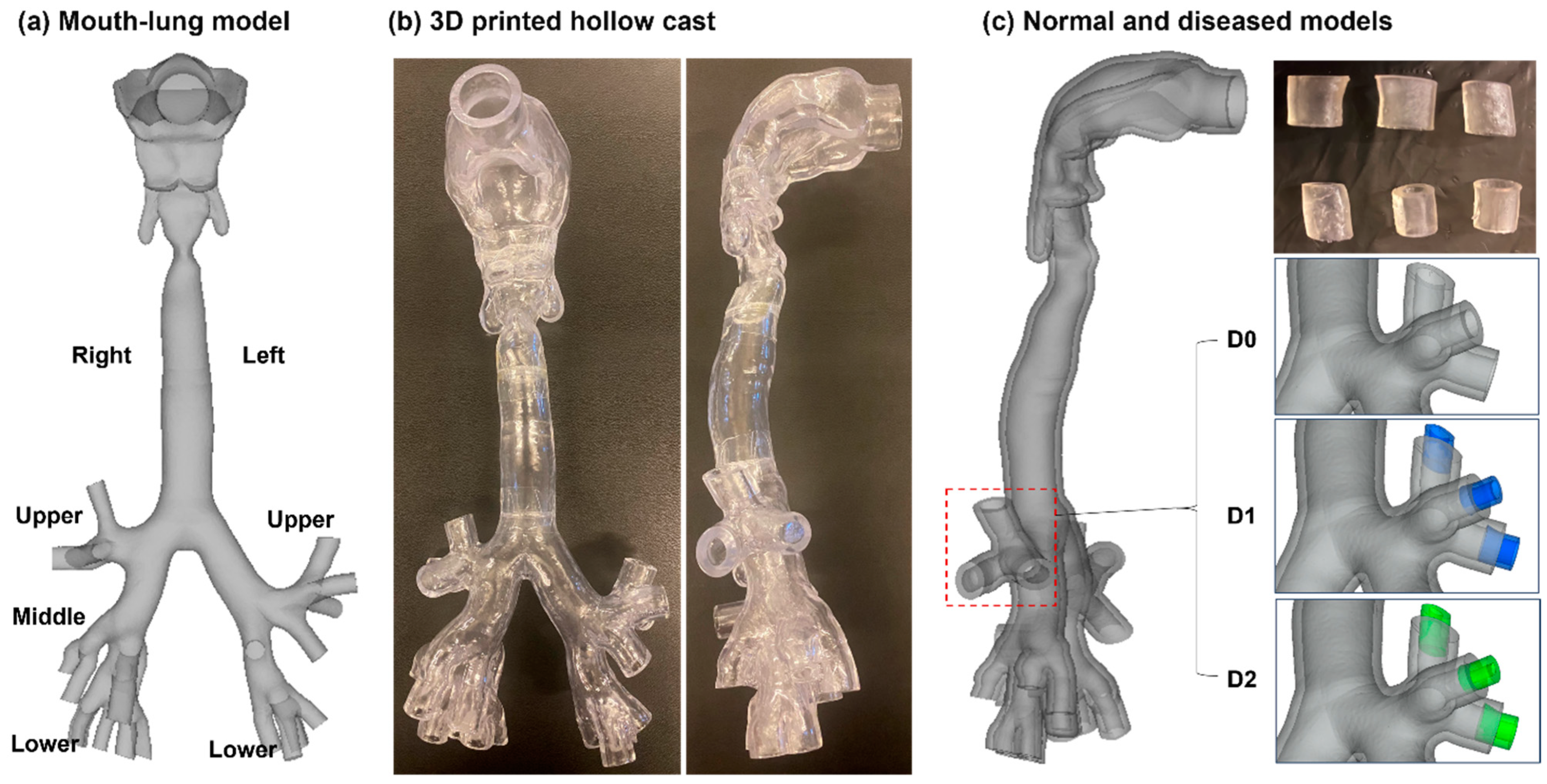
Develop normal and diseased lung models with mild and severe constrictions.
(2)
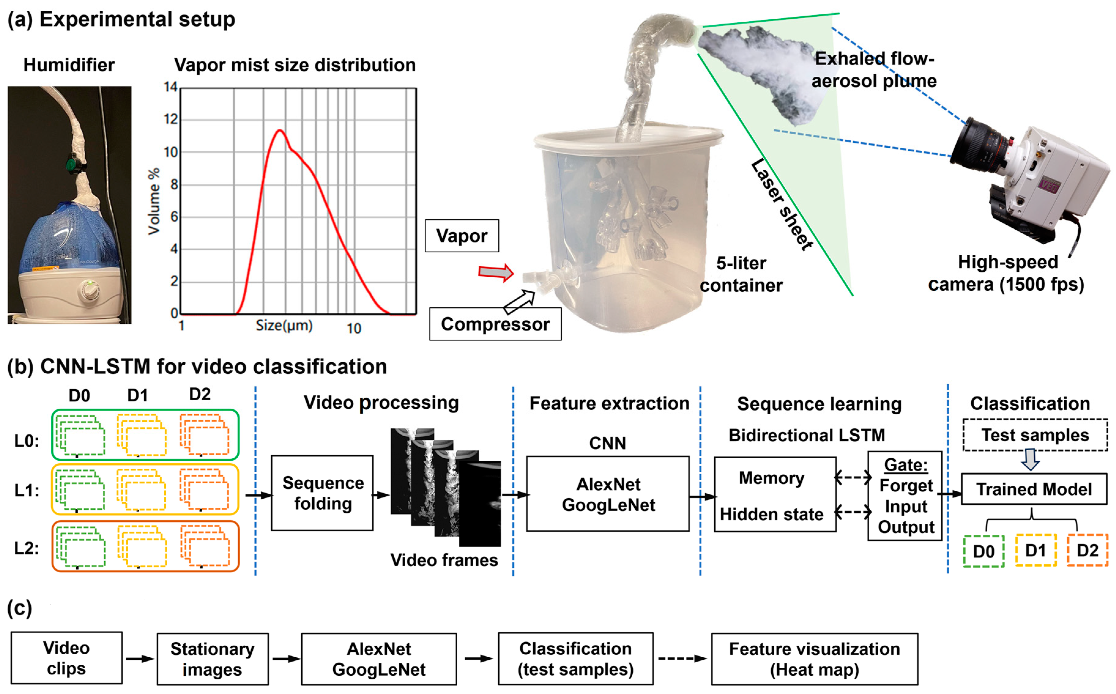
Record exhalation flows from the normal and diseased lung casts using a high-speed camera at 20, 15, and 10 L/min and analyze the flow videos using PIVlab.
(3)
Train two CNN-LSTM networks based on videos acquired at 20 L/min and test the networks using videos acquired at 20, 15, and 10 L/min.
(4)
Compare the classification performances based on videos and still images.
(5)
Calculate the categorial occlusion sensitivity for AlexNet and GoogLeNet.
The remaining text is organized as follows. In vitro models, the experimental setup, CNN-LSTM networks, and the study design are described in Section 2. The results of high-speed recording, PIVlab analyses, classification performance, and sequential and spatial features are presented in Section 3. The insights gleaned from this study are discussed in Section 4, with a concise conclusion in Section 5.

2. Materials and Methods

2.1. Normal and Diseased Lung Models

An image-based mouth–throat model, previously reported in [47], was utilized to examine exhalation flows. The model featured a round oral opening with a diameter of 20.8 mm, and its lung branching extended to the fifth generation (G5), as shown in Figure 1a. Initially derived from CT scans of a healthy adult male, the model’s dimensions, as well as the methods employed in its development, were detailed in [48].
To simulate lobar asthmatic conditions within the lung model, flow resistors with two reduced diameters were applied to the outlets of the tertiary bronchi in the right upper (RU) lobe. The diameter of the normal lung was 5.6 mm. Three-dimensionally printed resistors with a 4 mm inner diameter and 5.6 mm outer diameter were inserted into the RU tertiary bronchi to generate the first asthmatic lung model (D1), mimicking mild constriction due to muscle over-secretion and/or muscle inflammation. Similarly, resistors with a 2 mm inner diameter and 5.6 mm outer diameter were used to generate an asthmatic lung model (D2) with more severe constriction. The mouth–lung casts were prepared using a Form 3B+ 3D printer (Formlabs, Somerville, MA, USA) and a clear stereolithography (SLA) resin (Formlabs Clear Resin, FLGPCL04). To ensure a tight seal, a stepped groove was incorporated at the connecting ends of each part.

2.2. Experimental Setup

A 3D-printed mouth–lung cast was housed in a 5 L container (Figure 2a). The container was connected to two tubes: one for introducing a soft mist from an ultrasonic cool mist humidifier (Pure Enrichment, Huntington Beach, CA, USA) and the other for channeling airflow from a compressor (Chad 50 PSI, Port Washington, NY, USA). The output mists from the humidifier were measured using a laser diffraction droplet size analyzer (Spraylink, Dickinson, TX, USA), with D10, D50, and D90 being 2.95, 4.62, and 8.55 µm, respectively. The compressor’s flow rate was adjusted using a PWM Motor Speed Controller (Rio Rand, Fresno, CA, USA), allowing accurate control of the flow rate.
A Phantom 13100L high-speed camera (Ametek, Wayne, NJ, USA), capable of capturing up to 11,000 frames per second, recorded the exhaled flow with aerosol mists at 1500 fps (Figure 2a). A 100 mW, 488 nm laser sheet was used to ensure adequate illumination of the mist droplets for clear visualization. Exhaled mist patterns were systemically recorded from both the normal (D0) and two asthmatics (D1 and D2) at three flow rates (20, 15, and 10 L/min), corresponding to a mean velocity of 1.0, 0.75, and 0.5 m/s through a mouth outlet of 20.8 mm. The video recordings at 20 L/min were used to train the CNN-LSTM classifier, while those at 15 L/min and 10 L/min were used as deviants to test the robustness of the trained CNN-LSTM classifier. For each test condition (i.e., with a given lung model and flow rate), a recording of one minute or longer was taken, which was further segmented into 30 clips or so, with each clip lasting 2 s. Each test was repeated three times or more, generating at least 90 video clips for each test case. The network’s classification robustness to temporal features was also tested by shifting the video clips by 1 s.

2.3. CNN-LSTM Networks for Video Classification

2.3.1. CNN Models

The video classification of disease-specific exhaled flows consists of four phases, video processing, feature extraction, sequence learning, and classification, as shown in Figure 2b. In sequence folding, videos are parsed into a batch of images before any convolutional operations are performed. Two networks were considered in this study: AlexNet and GoogLeNet. Both models excel at image and video recognition. AlexNet was the 2012 winner of the ImageNet competition and comprises five convolutional layers followed by three fully connected layers [32,33]. GoogLeNet (or Inception) was the 2014 winner, known for its depth and width with reasonable computational resource requirements [49]. The inception modules allowed the optimization of filters of varying sizes at each layer and helped handle the variation in input information efficiently. Both networks extracted features from frames of the expiratory flow videos, capturing the distinct patterns of flow from the normal (D0) and two diseased (D1 and D2) lung models.

2.3.2. LSTM

LSTM is a type of recurrent neural network optimized for sequence prediction problems. In video classification, sequences of frames are fed into the network. By integrating LSTM with CNNs, the temporal dependencies between video frames can be captured. This is vital for understanding patterns in expiratory flows, which are inherently sequential. In doing so, each frame of the video is passed through either AlexNet or GoogLeNet to extract a high-dimensional vector (features) from each frame, followed as inputs into LSTM. After processing through the LSTM that learns the temporal dynamics of the expiratory flows, the final output is passed through a softmax layer (or any appropriate activation function) to classify the video as either ‘D0: normal’, ‘D1: mild asthmatic’, or ‘D2: severe asthmatic’, as shown in Figure 2b.
The core of the LSTM network consists of a BiLSTM layer with 2000 hidden units, recognizing patterns and sequences of patterns over the frames of a video, such as the progression of the mist plume or the trajectory of a vortex. The output from the LSTM layers can then be passed to a dense layer with SoftMax activation to produce classification probabilities for each category. During training, both the CNN and LSTM components can be trained together end-to-end using labeled video data. The network is optimized to minimize the difference between its predictions and the actual labels using a categorical cross-entropy loss to classify videos into specific categories.

2.3.3. Training Configuration and Performance Matrices

Optimal learning was facilitated through a mini-batch size of 16 and an initial learning rate of 0.0001. A gradient threshold of 2 was used to prevent potential issues with gradient explosion. Randomness was introduced by shuffling data at the start of each epoch. Furthermore, a once-per-epoch validation check was enforced to monitor the network’s efficiency.
Multiple metrics were calculated from the confusion matrix to assess the classification performance of the network. These included overall accuracy and categorical matrices such as precision, sensitivity, specificity, F1 score, ROC (receiver operating characteristic) curve, and AUC (area under the curve). In the case of three-class classification (namely D0, D1, D2), these categorical metrics were adapted from their binary versions, employing the One-vs-Rest (OvR) method, e.g., D0 vs. (D1 and D2), D1 vs. (D0 and D2), and D2 vs. (D0 and D1). More details of the methods to calculate the performance matrices can be found in [50].

2.3.4. Heat Map

Heatmap analyses were conducted to understand the network-learned features under different asthmatic severities. To obtain the heatmap, corresponding training and testing using the CNN models were also conducted using stationary images from the same training/testing video sets, with each 2 s long video clip being split into 3000 images. The ensuing comparison of classification performance between the CNN-LSTM and CNN only would shed light on the impact of LSTM’s sequence learning.

2.4. Study Design

To evaluate the robustness of the video-classification models, both AlexNet-LSTM and GoogLeNet-LSTM were trained on video clips acquired at 20 L/min but tested on videos acquired at three flow rates, 20 L/min, 15 L/min, and 10 L/min, representing a difficulty level of Level 0 (baseline), Level 1, and Level 2, respectively. A ten-fold cross-validation approach was used to train the model, with the dataset randomly divided into ten equal-sized subsets. Ten runs were conducted and, in turn, nine subsets were used for training and the reaming dataset was used for testing [51]. To compare the diagnostic ability between AlexNet-LSTM and GoogLeNet-LSTM, both accuracy and categorical matrices, such as precision, sensitivity, specificity, F1-Score, ROC curve, and AUC, were calculated for each model, particularly at the Level 2 difficulty. To evaluate the LSTM’s sequence learning effect on model performances, the video clips were split into still images, which were further used to train and test AlexNet and GoogLeNet. Heat maps designating the most important regions for model classification were found in terms of occlusion sensitivity for D0, D1, and D2 in both AlexNet and GoogLeNet.
Training and testing of the CNN-LSTM and CNN models were carried out on an AMD Ryzen 3960X 24-Core workstation equipped with 3.79 GHz processors, 256 GB RAM, and a 24 GB GPU (PNY NVIDIA GeForce RTX 3090). In this study, using around 224 video clips and 12,000 images, a single training cycle for one CNN model required about 8–10 h to complete.

3. Results

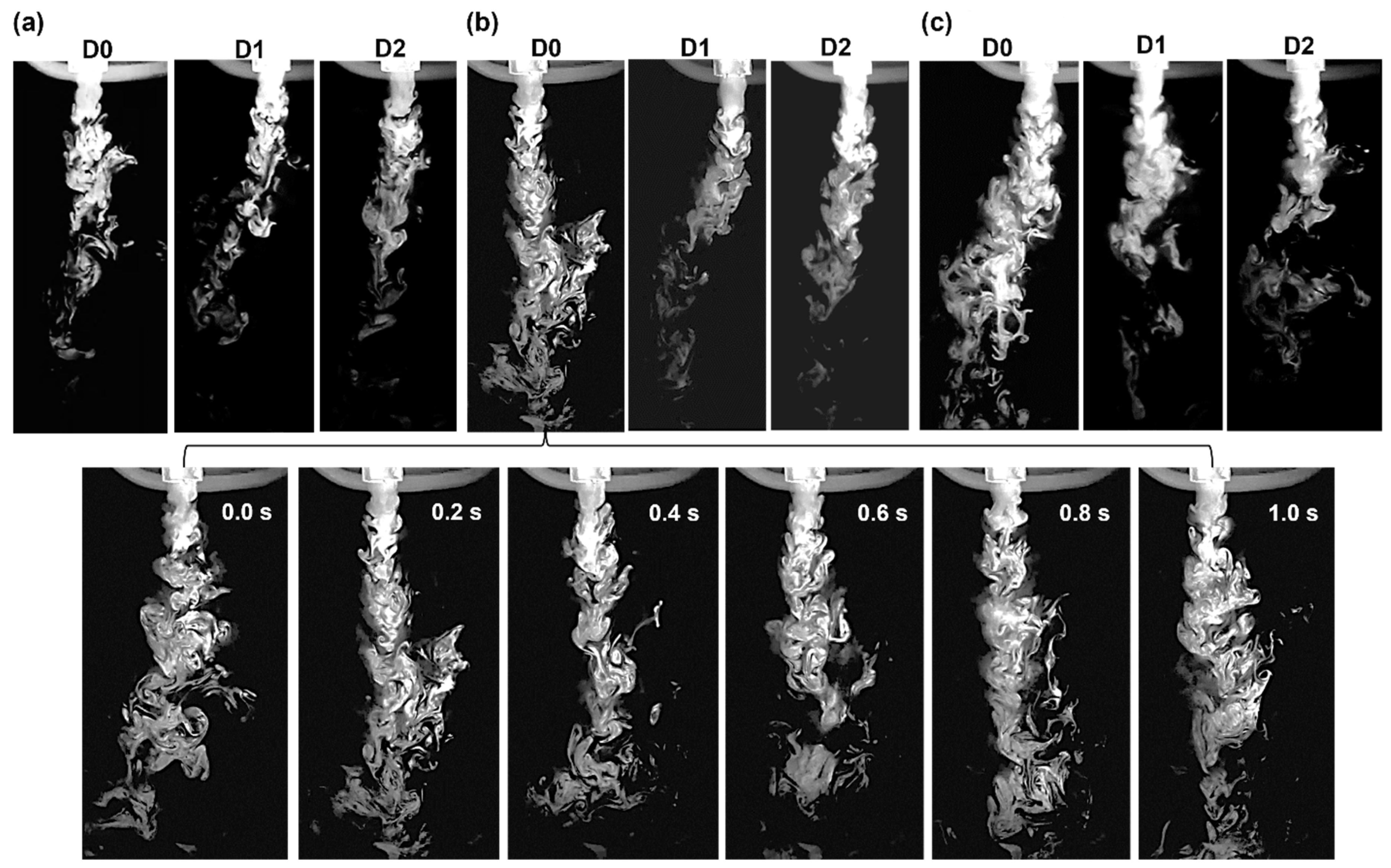
3.1. High-Speed Recording of Expiratory Flows

Figure 3 displays flow visualization images of exhaled breath from normal (D0) and diseased (D1, D2) lung models at different flow rates. High-resolution, yet highly complex, vortex patterns are observed in the mid-plane of the exhaled flows using the VEO high-speed camera acquired at 1500 fps. After exiting from the mouth, the exhaled flows quickly evolve into dense vortices due to the high-velocity flow jet. In addition, flow entrainment of ambient air occurs at the jet boundary, which decreases the plume speed and generates new vortices. These vortices are transported downstream by the main flow and, at the same time, experience stretching, decay, and compression along the journey. Note that even though these 2D mid-plane images only partially capture the dynamics of the 3D exhaled flow-aerosol plume, they are also advantageous in revealing details of the flow structures within the flow that a 3D plume cannot otherwise show. For different diseases and flow rates, the exhaled flows varied in penetration length, pattern complexity, vortex density, and sequential vortex evolution.
The effects of disease stage (D0, D1, D2) on exhaled flows can be evaluated at three exhalation flow rates (20, 15, and 10 L/min). The progression from healthy to disease states demonstrates a gradual decrease in flow penetration length. This change is presumably attributed to an increasing obstruction in the right upper lobe, which not only increases the flow resistance but also alters flow distribution among the five lobes, further elevating right–left asymmetry. In healthy lungs (D0), the vortex pattern appears to be more concentrated and complex, with vortices surviving for a longer time, accumulating along the axial direction and compressing previous vortices, while in diseased states (D1 and especially D2), the vortex flows are less vigorous and more diffuse.
The effects of flow rate on exhaled flows can be evaluated by comparing Figure 3a–c (i.e., 20 L/min, 15 L/min, and 10 L/min). At the highest flow rate (Figure 3a), there is a strong, fast jet of exhaled air. In healthy lungs, this jet is coherent and penetrates longer, whereas, in diseased states, particularly in D2, it is disrupted to the extent that it becomes less visible due to turbulent mixing. At lower flow rates (Figure 3b,c), the exhaled air has less kinetic energy, leading to a more stable vortex flow in D0, which evolves at a slower pace and remains visible for a longer time and distance. By contrast, the disruption to vortex flows due to disease (D1 and D2) remains noticeable at 15 and 10 L/min, with both cases maintaining perceivable diffusion and disorganization (Figure 3b,c).
The lower panel of Figure 3 displays a time sequence of expiratory flow from D0 at 15 L/min over the course of one second. Coherent flow structures persist over time. Even though the patterns vary with time-varying vortex sizes and rearrangements, the overall complexity, vortex density, and penetration length remain unchanged. Also note that the vortex complexity, or irregularity, is highly heterogeneous along the axial direction. Both the similarities and differences may contain anomaly-sensitive information, which can be further explored to detect diseases and estimate disease state.

3.2. PIVlab Analyses of Videos

3.2.1. Velocity and Vorticity

The videos were analyzed using PIVlab to explore the flow characteristics. Figure 4 shows the PIVlab-derived velocities and vorticities of the videos from D0, D1, and D2 at 20 L/min.
Note that the color bars used in D0, D1, and D2 in Figure 4a are different. The exiting velocity from the mouth in D0 is around 1.0 m/s, which is equivalent to a volume flow rate of 20 L/min, thus verifying the accuracy of the PIVlab analyses. It is also observed that the exhaled jet flow loses its kinetic energy to the ambient air, and its main flow velocity gradually decreases in the axial direction. The non-continuous red spots in the velocity maps indicate the instantaneously unstable main flows (Figure 4a).
The instantaneous vorticity maps corresponding to the above velocity contours are presented in Figure 4b. It is clearly shown that the flow regions with the highest vorticity intensity are not the same as the regions with high velocities. High-vorticity regions are observed at both the flow cores and boundaries, where a large velocity gradient exists.
Figure 4c compares the velocity distributions among D0, D1, and D2 along a transverse line (8 cm downstream of the mouth) and an axial line, respectively. It is observed that at 8 cm downstream of the mouth, the flow speed has decreased from 1 m/s at the mouth opening to approximately 0.5 m/s. Considering different disease states, the velocity in D0 is slightly higher than in D1 and D2. This observation corroborates with the higher flow resistances in D1 and D2 due to increasing obstructions in the right upper lobe. This pattern is also noted in the axial flow velocity variations (right panel, Figure 4c), where D0 is slightly higher than D1, and D1 is slightly higher than D2.

3.2.2. Vortex Locations

Figure 5 shows the instantaneous vortex locations corresponding to the velocity fields in the above figure both in the 2D map format (upper panel) and along the axial direction. Both the locations and numbers of vortices differ among different disease states. More importantly, how the vortex locations change with time, in both vortex locations and vortex densities, can be inherently correlated to underlying diseases. Vortices can play critical roles in mixing, momentum transfer, energy dissipation, and flow instability, thus having significant implications in establishing disease-flow correlations.

3.3. Video Classification

3.3.1. AlexNet-LSTM

The three-class classification performance matrices of AlexNet-LSTM are presented in Figure 6 in terms of precision, specificity, sensitivity, and F1 score. The same data are also listed in Table 1. All four matrices are class-specific (D0, D1, D2) and tested on video samples of three levels of difficulty (L0, L1, L2). The average and variance of each matrix were also calculated over the three levels and are presented as the fourth group in each figure. Note that the AlexNet-LSTM network was trained on L0 video (baseline, acquired at 20 L/min).
All matrices for video classification are 100% on L0 test samples (Figure 6a–d, which is not surprising considering the video similarities between the training and testing sets. This high performance serves as verification that the trained network has indeed captured disease-associated features. The video classification is also perfect when tested on the Level 1 dataset containing 100 2 s video clips acquired at 15 L/min, signifying that the network has indeed learned certain inherent features unique to the disease, which remain detectable despite a 25% deviation in the flow rate during video acquisition. However, a further flow deviation of 50% (from 20 L/min to 10 L/min) led to significant misclassifications, reducing the overall accuracy from 100% to 72.8%. All class-specific metrics decrease correspondingly. The average and variance of each matrix have also been calculated over three categories, D0–2, and are presented as the fourth group in Figure 6a–d. At Level 2 difficulty, the overall precision is 74.6% ± 11.7, sensitivity is 72.8 ± 21.5, specificity is 86.4 ± 8.8%, and F1 score is 71.6% ± 13.5.
The ROC (receiver operating characteristic) curves at Level 2 difficulty are also presented in Figure 6e, which plots the true positive rate (TPR) vs. the false positive rate (FPR) and illustrates the diagnostic ability of a network on a specific class at various threshold settings. It clearly shows the different abilities of the network in diagnosing D0, D1, and D2, indicating the challenges in identifying robust anomaly-sensitive features. The area under the curve (AUC) of the ROC is also presented in Figure 6e, providing a single scalar value to evaluate the performance. An AUC value of 1 for D0 suggests that the AlexNet-LSTM model has a perfect discrimination ability for D0 when tested on L2 test samples. By contrast, AUC values of 0.8281 for D1 and 0.8848 for D2 indicate that the AlexNet-LSTM model has a lower but satisfactory discriminative power for D1 and D2 at Level 2 difficulty. The model operating point is also presented for each ROC curve (Figure 6e). These points represent the compromise between TPR and FPR chosen for each case, capturing as many true positives as possible while keeping false positives reasonably low.

3.3.2. GoogLeNet-LSTM

Figure 7 and Table 2 show the three-class classification performance matrices of GoogLeNet-LSTM trained on L0 and tested on L0, L1, and L2 datasets. Similar to AlexNet-LSTM, the video classification by the GoogLeNet-LSTM network achieved 100% classification on the baseline datasets (L0), thus verifying the capture of defining features specific to the disease by the GoogLeNet-LSMT network. Unlike AlexNet-LSTM, misclassification by GoogelNet-LSTM starts to occur at Level 2 difficulty with a flow deviation of 25% during video acquisition (i.e., from 20 L/min to 15 L/min). The overall accuracy is 91.5%, the averaged sensitivity is 92.7%, and the specificity is 96.3%, which still provides a high classification performance on Level 1 data. However, a drastic decrease in classification is observed on Level 2 test videos (acquired at 10 L/min), with an overall accuracy of 57.7%, a cross-class averaged sensitivity of 57.7% ± 33.0%, and a specificity of 78.9% ± 15.2%.
Class-specific ROC curves of GoogLeNet-LSTM are shown in Figure 7e. For Level 1 difficulty (upper panel, Figure 7e), all ROC curves are close to the left upper corner, with AUC values of 0.998–1.0, initiating high diagnostic abilities at this level. However, at Level 2 difficulty (lower panel, Figure 7e), the ROC curves for D1 and D2 are close to the diagonal of the graph, with low AUC values of 0.70–0.71, indicating an inadequate diagnostic ability of the network for video images acquired at 10 L/min.

3.3.3. Comparison between AlexNet-LSTM and GoogLeNet-LSTM

A comparison of the three-class performance matrices between the two networks is presented in Figure 8. In Figure 8a, the advantage of using AlexNet-LSTM over GoogLeNet-LSTM increases with increasing levels of difficulty (or flow deviation), suggesting a superior robustness of the AlexNet-LSTM network than GoogLeNet-LSTM. Considering the class-specific matrices such as precision, sensitivity, specificity, and F1 score, AlexNet-LSTM exhibits much higher performance than GoogLeNet-LSTM for the two disease cases D1 and D2, while showing an equivalent or slightly lower performance for the normal case D0 (Figure 8). This observation holds for both Level 1 and Level 2 datasets, suggesting that AlexNet-LSTM has captured more fundamental features associated with the disease-induced structural variations than GoogLeNet-LSTM, even though it is still unclear whether these features are spatial or temporal. A similar finding is also observed in Figure 8d, where the ROC curves for D1 and D2 at Level 2 difficulty clearly demonstrate a substantial superiority of AlexNet-LSTM (solid lines) over GoogLeNet-LSTM (dashed lines).

3.4. Sequential Effects in Classification

3.4.1. Time Shifting in Video Classification

Considering that the LSTM network learns sequential information from the videos, we wish to test how the diagnostic ability of the CNN-LSTM networks varies if the 2 s test video clips were shifted by 1 s. To accomplish this, the Level 1 video clips were shifted by 1 s (i.e., L1-1s) and retested, with the resulting performance matrices listed in Table 1 and Table 2. For AlexNet-LSTM, the classification on L1-1s is perfect in each matrix, mirroring the results obtained from L1 video samples. For AlexNet-LSTM, the difference is less than 2% for all matrices considered, indicating that shifting the test videos by 1 s has an insignificant impact on one classification result. Also note that in this study, videos were acquired at constant flow rates, generating similar, if not time-invariant, flow features; thus, shifting one 2 s video by 1 s does not add or reduce information and should not significantly affect the classification results.

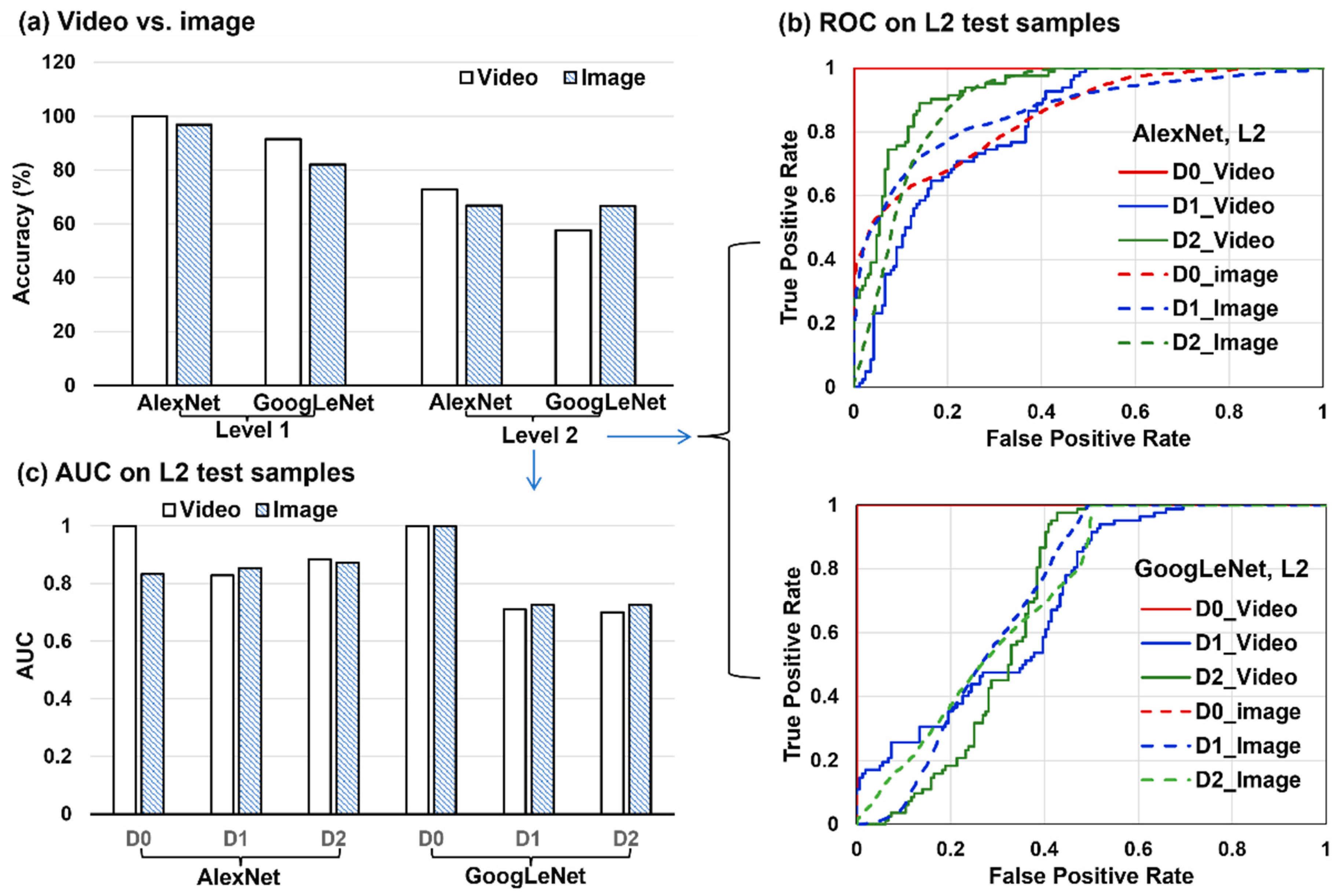
3.4.2. Videos vs. Still Images

To assess the effects of using videos and still images on classification performance, each video clip was split into still images and was trained and tested using AlexNet and GoogLeNet (without LSTM). Figure 9a shows the resultant classification accuracies in comparison to their LSTM counterparts, tested on L1 and L2 datasets. Detailed image classification matrices for AlexNet and GoogLeNet are listed in Table 3 and Table 4, respectively. For both levels (L1 and L2), video classifications outperformed classifications with still images. Similar to video classifications, AlexNet slightly outperforms GoogLeNet on images, especially on Level 2 acquired with a larger flow deviation (10 L/min vs. baseline of 20 L/min).
Figure 9b compares the video- and image-based ROC profiles at various threshold settings for the classification task at Level 2 difficulty. It is observed that for AlexNet networks, the video inputs consistently have a higher true positive rate across almost all false positive rates, indicating better performance. The lines for video inputs (solid lines) are generally above those for image inputs (dashed lines), with D0 having the highest performance (closest to the top-left corner), followed by D1 and D2. More complex trends are observed for GoogLeNet networks, with ROC curves mingling between videos and still images. In comparison to the AlexNet ROC curves closer to the top-left corner of the graph, GoogLeNet’s ROC curves are closer to the diagonal of the graph, suggesting an overall lower performance of GoogLeNet models when tested at Level 2 difficulty.
The areas under the curve (AUCs) of the ROC curves in Figure 9b are shown in Figure 10b. Considering AlexNet, a much higher AUC value is noted for D0 with video inputs compared with still images, while insignificant differences between videos and images are noted for D1 and D2, which lead to a cumulatively better performance with videos than images. On the other hand, when tested at Level 2 difficulty, GoogLeNet gives an equivalent AUC on D0 images but lower AUC values on D1 and D2 imaging, leading to an overall inferior classification for videos than still images, consistent with a lower video accuracy in Figure 9a and intermingling video/image ROC curves in Figure 6b.

3.5. CNN Learned Spatial Features from Still Images

3.5.1. AlexNet

In machine learning, particularly in the field of computer vision, an occlusion sensitivity map is a technique used to understand which parts of an input image are most important for a neural network’s predictions (Figure 10). This is carried out by systematically occluding (covering up) different parts of the input image and then measuring how much the network’s predictions change. If a small occlusion causes a significant change in the prediction, the occluded area is likely important for the network’s decision making.
The upper row of Figure 10 compares the occlusion sensitivity map obtained from AlexNet. The heat map for a normal lung (D0) is only observed at the mouth opening and is less pronounced than those in D1 and D2 (Figure 10a vs. Figure 10b,c), indicating fewer areas of high sensitivity. This is consistent with the expectation that a normal lung would not exhibit significant features indicative of asthma and that AlexNet relies mainly on flow features at the mouth opening, concluding that the lung is normal. The occlusion map in Figure 10b shows a more pronounced heat map around 5 cm downstream of the mouth opening, signifying the flow region where occlusion has a defining impact in identifying D1 (mild asthma). A double-zone heat map is observed for D2, indicating that the model finds more variations in the flow features, when occluded, substantially affecting its ability to recognize severe asthma.

3.5.2. GoogLeNet

Distinct patterns in the occlusion sensitivity map are found in GoogLeNet compared to AlexNet (lower row vs. upper row, Figure 10). No focused heat map is found in the lower panel of Figure 10a, indicating that GoogLeNet is not particularly sensitive to any specific occlusions, reflecting that the flows from the normal lung do not contain strong features associated with asthma. In mild asthmatic cases (D1, lower panel, Figure 10b), the sensitivity map starts to show areas where occlusions change the model’s predictions, highlighting the flow patterns related to the mild asthmatic features. For severe asthmatic cases (D2, lower panel, Figure 10c), the occlusion sensitivity map shows a more focused heat map, indicating a strong sensitivity of GoogLeNet to occlusions in this area in identifying severe asthma.

4. Discussion

By leveraging CNN’s feature extraction with LSTM’s sequence learning, this study evaluated the feasibility of using exhaled flows to detect constrictive lung diseases and stage the disease severity. Interesting differences were observed regarding the performances of AlexNet-LSTM vs. GoogLeNet-LSTM, video-based vs. image-based classification, and the proposed flow-based diagnostic method vs. previous techniques, as discussed below in detail.

4.1. AlexNet-LSTM vs. GoogLeNet-LSTM

High performances were obtained with AlexNet-LSTM in three-class classification across all flow conditions (Level 0–2). The network was trained on Level 0 (baseline, 20 L/min) test videos, which achieved 100% classification for the three categories (D0, D1, D2) across all metrics—accuracy, precision, specificity, sensitivity, and F1-Score. A similar perfect score was maintained for Level 1 test videos (15 L/min), which were acquired at 15 L/min. Even when the Level 1 video clips were shifted by 1 s, the hybrid AlexNet-LSTM performance remained unchanged, upholding its 100% classification across all metrics (Table 1). However, a decline was noted at Level 2 difficulty (i.e., videos acquired at 10 L/min), with the accuracy tapered to 72.8%, sensitivity to 72.7%, specificity to 86.4%, and F1-Score to 71.6.0% (Figure 6 and Table 1 and Table 3). The F1 score merges Precision and Recall into one metric, providing a comprehensive measure of a binary classification model’s effectiveness. A high F1 score reflects robust overall performance, indicating the model’s proficiency in accurately identifying positive cases with a low rate of both false positives and false negatives. Despite the large deviation in Level 2 flow rate from the baseline (i.e., 10 L/min vs. 20 L/min), the hybrid AlexNet-LSTM network still provides adequate classification performance, indicating a robust model for lung disease diagnosis from exhaled flow videos.
At Level 0 difficulty, both the GoogLeNet-LSTM and AlexNet-LSTM networks achieved perfect performance, suggesting that either model could be selected without preference when analyzing test videos recorded under optimal breathing conditions. From Level 1 (15 L/min), GoogleNet-LSTM started to show a reduction in categorical precision (73.1% for D0) and sensitivity (78.1% for D3), indicating an increased rate of false positives and false negatives, even though its combined accuracy remained high (91.5%, Table 2). On the other hand, AlexNet-LSTM continued to perform perfectly at Level 1, even when the test video clips shifted by 1 s.
The real challenge for both networks arose at Level 2 difficulty (10 L/min). Both networks showed significantly lower accuracy and categorical F1 scores (Table 1 and Table 2 and Figure 8), indicating that an increased flow deviation challenged their ability to capture the morphology-related information, leading to increased false positives. The performance of GoogleNet-LSTM showed a more noticeable decline compared to that of AlexNet-LSTM; thus, the AlexNet-LSTM network was more robust to flow rate uncertainties for this classification task, despite GoogLeNet having a more complex architecture and deeper layers than AlexNet. Neither network was able to maintain its Level 0 performance as the flow rate deviated from the training set condition, highlighting the necessity of breath tests under standardized breathing conditions during video acquisition.

4.2. Video-Based vs. Image-Based Classifications

In this study, we compared the performance matrices between video-based and image-based classification tasks on three testing datasets with increasing levels of difficulty (i.e., baseline 20 L/min, 15 L/min, and 10 L/min), as listed in Figure 9 and Table 1, Table 2, Table 3 and Table 4. When trained and tested on the baseline dataset, both video and image classifications gave 100% accuracy, suggesting that the spatial features extracted from images were sufficient to distinguish the disease state, even without resorting to temporal features. In other words, both the CNN-LSTM and CNN-only networks succeeded in capturing disease-sensitive features.
However, when the acquisition flow rate deviated from the baseline, the advantage of sequence learning became noticeable. Considering AlexNet, the video-based accuracy is 3.1% higher at Level 1 difficulty (100% vs. 96.9%, Figure 9a) and is 6.0% higher at Level 2 difficulty (72.8% vs. 66.8%). Three points are noteworthy. First, video classification outperformed image classification at both levels, and the advantages of sequence learning became more obvious when tested on more adverse conditions. Second, for this classification task, sequence learning exerted a larger positive effect on AlexNet than on GoogLeNet, as illustrated in Figure 9b. Thirdly, videos were acquired under constant exhalation flow conditions, and the temporal flow features, despite their fluctuation, were statistically temporally invariant (analogous to oscillations over a horizontal line). This explained the improved accuracies of CNN-LSTM over CNN, yet with an insignificant magnitude. It is envisioned that videos of exhaled flows under tidal flow conditions contain more temporal information, and an even larger enhancement in classification performance is expected from CNN-LSTM networks than their CNN counterparts.

4.3. Lung Diagnosis Using Exhaled Flows vs. Other Methods

Impulse oscillometry (IOS) utilizes low-frequency sound waves (5–20 Hz) to measure the mechanical properties of the airway, including resistance (R), compliance (C), and inertia (I). As the wave passes into the lungs, it causes pressure changes in the flow of the air. The frequency-specific properties will help locate the disease site, i.e., the high frequency being related to the upper, large airways and the low frequency to lower, small airways [52]. However, further evidence is required to establish its clinical utility [53]. In vitro studies of IOS were often limited by the rigid 3D-printed lung casts that excluded the compliance of the lung [22]. Even with the recent advent of 3D printing techniques allowing elastic materials, preparing a mouth–lung replica cast that realistically simulates the site-dependent compliance of the respiratory system is still highly challenging, if not impossible. By contrast, exhaled-flow videos contain more information than the single values of resistance/compliance/inertance provided by IOS. Particularly, time-dependent information can reveal instantaneous interactions between the exhaled flows and the respiratory tract structure, yielding quick, time-varying flow fields and vortex dynamics. As shown in Figure 3, Figure 4 and Figure 5, different disease states (D0–2) generated distinct patterns of flows and vortices, manifested as differences in the flow plume penetration length, vortex complexity, and vortex decay rate. Either by handcrafting features with known disease correlation or leveraging CNN’s automatic feature extraction, the time-varying flow characteristics promise to disclose more information about lung health, especially the disease site, location, and severity.
The aerosol bolus disperser technique (ADB) also utilizes time-varying information on exhalation flows but is limited to the variation in aerosol concertation vs. expiratory flow volume. This technique is an ensemble approach that integrates transient flow-aerosol variations into a single parameter (aerosol concentration). Thus, combining these methods, which consider both the aerosol concentration and the instantaneous flow/vortex dynamics, is expected to provide a more effective synergic tool for lung diagnosis.
Breathomics analyzes exhaled gases (volatile and nonvolatile) or condensates and has been proven to be effective in detecting the presence and severity of certain diseases [54,55]. This method relies on the variation in breath metabolites that can indicate various disease states, not the airway structural remodeling. Thus, the flow-based method proposed in this study can act as a complementary tool to the breathomics approach in detecting respiratory pathologies by looking into variations in both lung tissue metabolism and airway morphology/integrity.
In the past several years, we also explored the usages of 2D images of exhaled aerosol distributions collected on filters at the mouth opening for obstructive lung diagnosis using either handcrafted features [51,56] or CNN networks [57,58]. These methods are similar to the newly proposed technique hereof in that both approaches leverage the unique flow-aerosol dynamics after interacting with a remodeled lung structure. The difference lies in the fact that filter-collected aerosol images are stationary, 2D, and cumulative in nature, while the videos of exhaled flows and entrained aerosols are dynamic, 3D, and time-varying, whose wealth of information promises to better reveal the underlying lung diseases.
Foreseeable obstacles exist to this newly proposed lung diagnostic method. First, the sensitivity of exhaled flows to airway remodeling, as well as its impact on classification accuracy, has not yet been explored, particularly when the airway remodeling is small in size. Second, the airway remodeling was in the right upper (UR) lobe in this study. The classification task can be more challenging when the remodeling occurs in small airways. However, it is also noted that high classification accuracies were obtained with the UR lobar constrictions, even when the acquisition flow rates deviated from baseline by 50%. It is thus still very likely to achieve the desired diagnostic accuracy for small airway diseases by following recommended protocols, including the recommended flow maneuver.

4.4. Limitations and Future Studies

This study can be further improved by several factors. First, constant flow rates are used during video recording in this feasibility exploratory study. Tidal flows with a prescribed breathing maneuver will be more clinically relevant and yield more complex, temporally varying flow patterns [48,59]. The overall fluctuating but temporally invariant flow patterns explained the marginal improvement in the hybrid CNN-LSTM approaches using videos over their CNN counterparts using still images. The LSTM’s sequence learning is expected to take in more information on the flow evolution within the exhalation cycle and aid the classification of the disease states. Second, the mouth–lung casts were made from rigid materials and did not consider tissue compliance or dynamic structures during respiration, like the lip, tongue, glottis, and pharynx, which can modify expiratory flow dynamics [60,61,62,63,64,65]. Having said that, it is also noted that as long as the videos are acquired in a consistent manner (i.e., disease state being the sole variable with all other influencing factors fixed), the classification results will be sufficiently indicative of the method’s feasibility while significantly reducing the experimental complexity. Only one patient’s lung model was considered; including more lung models can inform us about the intersubject variability. The training dataset contained 224 video clips, equaling 13,440 still images. Increasing the sample size will enable the networks to learn more disease-sensitive features and thus have the potential to increase the classification performance further. Finally, only two pre-trained CNN models (AlexNet and GoogLeNet) were considered based on their proven superior performance vs. relative simplicity [49,50]. To identify one optimal CNN for this classification task, more recent approaches need to be evaluated, which are either with more advanced architectures and deeper layers, such as ResNet50 [66] and VGG19 [67], or with simpler architectures and being more time efficient, such as MobileNet [68] and EfficientNet [69].

5. Conclusions

This study evaluated the feasibility of using the video classification of exhaled flows for lung diagnosis by leveraging LSTM’s sequential learning capacity and CNN’s automatic feature extraction. The results showed that video inputs were observed to give higher diagnostic accuracies than image inputs. The AlexNet-LSTM network slightly outperformed the GoogleNet-LSTM network and was robust to reasonable breathing deviations during data acquisition. The union of deep learning and physiology-based in vitro modeling is promising to disclose anomaly-sensitive features amenable to non-invasive lung diagnosis. It was noted that this study used in vitro lung models with constant exhalation, which had the advantage of controlled asthmatic constrictions. Future studies were needed to consider the more physiologically realistic scenarios such as tidal breathing, compliant airways, and varying disease sites.

Author Contributions

Conceptualization, M.T., X.S. and J.X.; methodology, M.T., X.S. and J.X.; software, M.T. and J.X.; validation, X.S. and J.X.; formal analysis, M.T., X.S. and J.X.; investigation, M.T., X.S. and J.X.; data curation, M.T.; writing—original draft preparation, J.X.; writing—review and editing, M.T. and X.S.; visualization, M.T. and J.X.; supervision, J.X. All authors have read and agreed to the published version of the manuscript.

Funding

This research received no external funding.

Institutional Review Board Statement

Not applicable.

Informed Consent Statement

Not applicable.

Data Availability Statement

The data presented in this study are available upon request from the corresponding author.

Acknowledgments

Amr Seifelnasr at UMass Lowell Biomedical Engineering is gratefully acknowledged for constructive discussion and critical reviewing of this manuscript.

Conflicts of Interest

The authors declare no conflict of interest.

References

  1. Ibrahim, W.; Carr, L.; Cordell, R.; Wilde, M.J.; Salman, D.; Monks, P.S.; Thomas, P.; Brightling, C.E.; Siddiqui, S.; Greening, N.J. Breathomics for the clinician: The use of volatile organic compounds in respiratory diseases. Thorax 2021, 76, 514–521. [Google Scholar] [CrossRef]
  2. Miekisch, W.; Schubert, J.K.; Noeldge-Schomburg, G.F.E. Diagnostic potential of breath analysis—Focus on volatile organic compounds. Clin. Chim. Acta 2004, 347, 25–39. [Google Scholar] [CrossRef]
  3. Kostikas, K.; Koutsokera, A.; Papiris, S.; Gourgoulianis, K.I.; Loukides, S. Exhaled breath condensate in patients with asthma: Implications for application in clinical practice. Clin. Exp. Allergy 2008, 38, 557–565. [Google Scholar] [CrossRef] [PubMed]
  4. Loukides, S.; Bakakos, P.; Kostikas, K. Oxidative Stress in Patients with COPD. Curr. Drug Targets 2011, 12, 469–477. [Google Scholar] [CrossRef] [PubMed]
  5. Colombo, C.; Faelli, N.; Tirelli, A.S.; Fortunato, F.; Biffi, A.; Claut, L.; Cariani, L.; Dacco, V.; Prato, R.; Conese, M. Analysis of inflammatory and immune response biomarkers in sputum and exhaled breath condensate by a multi-parametric biochip array in cystic fibrosis. Int. J. Immunopathol. Pharmacol. 2011, 24, 423–432. [Google Scholar] [CrossRef]
  6. Vijverberg, S.J.H.; Koenderman, L.; Koster, E.S.; van der Ent, C.K.; Raaijmakers, J.A.M.; Maitland-van der Zee, A.H. Biomarkers of therapy responsiveness in asthma: Pitfalls and promises. Clin. Exp. Allergy 2011, 41, 615–629. [Google Scholar] [CrossRef] [PubMed]
  7. Mazzone, P.J. Analysis of volatile organic compounds in the exhaled breath for the diagnosis of lung cancer. J. Thorac. Oncol. 2008, 3, 774–780. [Google Scholar] [CrossRef]
  8. Buszewski, B.; Kesy, M.; Ligor, T.; Amann, A. Human exhaled air analytics: Biomarkers of diseases. Biomed. Chromatogr. 2007, 21, 553–566. [Google Scholar] [CrossRef] [PubMed]
  9. Horvath, I.; Lazar, Z.; Gyulai, N.; Kollai, M.; Losonczy, G. Exhaled biomarkers in lung cancer. Eur. Respir. J. 2009, 34, 261–275. [Google Scholar] [CrossRef]
  10. Phillips, M.; Cataneo, R.N.; Cummin, A.R.C.; Gagliardi, A.J.; Gleeson, K.; Greenberg, J.; Maxfield, R.A.; Rom, W.N. Detection of lung cancer with volatile markers in the breath. Chest 2003, 123, 2115–2123. [Google Scholar] [CrossRef]
  11. Khoubnasabjafari, M.; Mogaddam, M.R.A.; Rahimpour, E.; Soleymani, J.; Saei, A.A.; Jouyban, A. Breathomics: Review of sample collection and analysis, data modeling and clinical applications. Crit. Rev. Anal. Chem. 2022, 52, 1461–1487. [Google Scholar] [CrossRef] [PubMed]
  12. Blanchard, J.D. Aerosol bolus dispersion and aerosol-derived airway morphometry: Assessment of lung pathology and response to therapy, Part 1. J. Aerosol Med.-Depos. Clear. Eff. Lung 1996, 9, 183–205. [Google Scholar] [CrossRef] [PubMed]
  13. Goo, J.; Kim, C.S. Analysis of aerosol bolus dispersion in a cyclic tube flow by finite element method. Aerosol Sci. Technol. 2001, 34, 321–331. [Google Scholar] [CrossRef]
  14. Lee, D.; Lee, J. Dispersion of aerosol bolus during one respiratory cycle in a model lung airway. J. Aerosol Sci. 2002, 33, 1219. [Google Scholar] [CrossRef]
  15. Schulz, H.; Eder, G.; Heyder, J. Lung volume is a determinant of aerosol bolus dispersion. J. Aerosol Med. 2003, 16, 255–262. [Google Scholar] [CrossRef] [PubMed]
  16. Kohlhäufl, M.; Brand, P.; Scheuch, G.; Meyer, T.; Schulz, H.; Häussinger, K.; Heyder, J. Aerosol morphometry and aerosol bolus dispersion in patients with CT-determined combined pulmonary emphysema and lung fibrosis. J. Aerosol Med. 2000, 13, 117–124. [Google Scholar] [CrossRef]
  17. Shaker, S.B.; Maltbaek, N.; Brand, P.; Haeussermann, S.; Dirksen, A. Quantitative computed tomography and aerosol morphometry in COPD and alpha1-antitrypsin deficiency. Eur. Respir. J. 2005, 25, 23–30. [Google Scholar] [CrossRef]
  18. Sturm, R. Theoretical diagnosis of emphysema by aerosol bolus inhalation. Ann. Transl. Med. 2017, 5, 154. [Google Scholar]
  19. Brand, P.; App, E.M.; Meyer, T.; Kur, F.; Müller, C.; Dienemann, H.; Reichart, B.; Fruhmann, G.; Heyder, J. Aerosol bolus dispersion in patients with bronchiolitis obliterans after heart-lung and double-lung transplantation. The Munich Lung Transplantation Group. J. Aerosol Med. 1998, 11, 41–53. [Google Scholar] [CrossRef]
  20. Kohlhäufl, M.; Brand, P.; Rock, C.; Radons, T.; Scheuch, G.; Meyer, T.; Schulz, H.; Pfeifer, K.J.; Häussinger, K.; Heyder, J. Noninvasive diagnosis of emphysema. Aerosol morphometry and aerosol bolus dispersion in comparison to HRCT. Am. J. Respir. Crit. Care Med. 1999, 160, 913–918. [Google Scholar] [CrossRef]
  21. Hardy, K.G.; Gann, L.P.; Tennal, K.B.; Walls, R.; Hiller, F.C.; Anderson, P.J. Sensitivity of aerosol bolus behavior to methacholine-induced bronchoconstriction. Chest 1998, 114, 404–410. [Google Scholar] [CrossRef]
  22. Si, X.; Xi, J.S.; Talaat, M.; Donepudi, R.; Su, W.-C.; Xi, J. Evaluation of impulse oscillometry in respiratory airway casts with varying obstruction phenotypes, locations, and complexities. J. Respir. 2022, 2, 44–58. [Google Scholar] [CrossRef]
  23. Erfanian Ebadi, S.; Krishnaswamy, D.; Bolouri, S.E.S.; Zonoobi, D.; Greiner, R.; Meuser-Herr, N.; Jaremko, J.L.; Kapur, J.; Noga, M.; Punithakumar, K. Automated detection of pneumonia in lung ultrasound using deep video classification for COVID-19. Inform. Med. Unlocked. 2021, 25, 100687. [Google Scholar] [CrossRef]
  24. Shea, D.E.; Kulhare, S.; Millin, R.; Laverriere, Z.; Mehanian, C.; Delahunt, C.B.; Banik, D.; Zheng, X.; Zhu, M.; Ji, Y.; et al. Deep learning video classification of lung ultrasound features associated with pneumonia. In Proceedings of the 2023 IEEE Computer Society Conference on Computer Vision and Pattern Recognition Workshops (CVPRW)(CVPRW), Vancouver, BC, Canada, 17–24 June 2023; pp. 3103–3112. [Google Scholar]
  25. Bruno, A.; Ignesti, G.; Salvetti, O.; Moroni, D.; Martinelli, M. Efficient lung ultrasound classification. Bioengineering 2023, 10, 555. [Google Scholar] [CrossRef]
  26. Chui, K.T.; Gupta, B.B.; Liu, R.W.; Zhang, X.; Vasant, P.; Thomas, J.J. Extended-range prediction model Using NSGA-III optimized RNN-GRU-LSTM for driver stress and drowsiness. Sensors 2021, 21, 6412. [Google Scholar] [CrossRef]
  27. Barros, B.; Lacerda, P.; Albuquerque, C.; Conci, A. Pulmonary COVID-19: Learning spatiotemporal features combining CNN and LSTM networks for lung ultrasound video classification. Sensor 2021, 21, 5486. [Google Scholar] [CrossRef] [PubMed]
  28. Xi, J.; Si, X.A.; Kim, J.; Mckee, E.; Lin, E.-B. Exhaled aerosol pattern discloses lung structural abnormality: A sensitivity study using computational modeling and fractal analysis. PLoS ONE 2014, 9, e104682. [Google Scholar] [CrossRef] [PubMed]
  29. Karpathy, A.; Toderici, G.; Shetty, S.; Leung, T.; Sukthankar, R.; Fei-Fei, L. Large-scale video classification with convolutional neural networks. In Proceedings of the IEEE Conference on Computer Vision and Pattern Recognition (CVPR), Columbus, OH, USA, 23–28 June 2014; pp. 1725–1732. [Google Scholar]
  30. Zhang, X.; Yang, Y.; Shen, Y.W.; Zhang, K.R.; Ma, L.T.; Ding, C.; Wang, B.Y.; Meng, Y.; Liu, H. Quality of online video resources concerning patient education for neck pain: A YouTube-based quality-control study. Front. Public Health 2022, 10, 972348. [Google Scholar] [CrossRef]
  31. ur Rehman, A.; Belhaouari, S.B.; Kabir, M.A.; Khan, A. On the use of deep learning for video classification. Appl. Sci. 2023, 13, 2007. [Google Scholar] [CrossRef]
  32. Chen, J.; Wang, J.; Yuan, Q.; Yang, Z. CNN-LSTM model for recognizing video-recorded actions performed in a traditional chinese exercise. IEEE J. Transl. Eng. Health Med. 2023, 11, 351–359. [Google Scholar] [CrossRef] [PubMed]
  33. Senyurek, V.Y.; Imtiaz, M.H.; Belsare, P.; Tiffany, S.; Sazonov, E. A CNN-LSTM neural network for recognition of puffing in smoking episodes using wearable sensors. Biomed. Eng. Lett. 2020, 10, 195–203. [Google Scholar] [CrossRef]
  34. Gilik, A.; Ogrenci, A.S.; Ozmen, A. Air quality prediction using CNN+LSTM-based hybrid deep learning architecture. Environ. Sci. Pollut. Res. Int. 2022, 29, 11920–11938. [Google Scholar] [CrossRef] [PubMed]
  35. Li, C.; Zhang, Y.; Weng, Y.; Wang, B.; Li, Z. Natural language processing applications for computer-aided diagnosis in oncology. Diagnostics 2023, 13, 286. [Google Scholar] [CrossRef] [PubMed]
  36. Whata, A.; Chimedza, C. Deep Learning for SARS COV-2 Genome Sequences. IEEE Access 2021, 9, 59597–59611. [Google Scholar] [CrossRef] [PubMed]
  37. Khatun, M.A.; Yousuf, M.A.; Ahmed, S.; Uddin, M.Z.; Alyami, S.A.; Al-Ashhab, S.; Akhdar, H.F.; Khan, A.; Azad, A.; Moni, M.A. Deep CNN-LSTM with self-attention model for human activity recognition using wearable sensor. IEEE J. Transl. Eng. Health Med. 2022, 10, 2700316. [Google Scholar] [CrossRef] [PubMed]
  38. Qin, P.; Li, H.; Li, Z.; Guan, W.; He, Y. A CNN-LSTM car-following model considering generalization ability. Sensors 2023, 23, 660. [Google Scholar] [CrossRef] [PubMed]
  39. Sun, J.; Di, L.; Sun, Z.; Shen, Y.; Lai, Z. County-level soybean yield prediction using deep CNN-LSTM model. Sensors 2019, 19, 4363. [Google Scholar] [CrossRef] [PubMed]
  40. Gao, G.; Wang, C.; Wang, J.; Lv, Y.; Li, Q.; Ma, Y.; Zhang, X.; Li, Z.; Chen, G. CNN-Bi-LSTM: A complex environment-oriented cattle behavior classification network based on the fusion of CNN and Bi-LSTM. Sensors 2023, 23, 7714. [Google Scholar] [CrossRef]
  41. Lu, W.; Rui, H.; Liang, C.; Jiang, L.; Zhao, S.; Li, K. A method based on GA-CNN-LSTM for daily tourist flow prediction at scenic spots. Entropy 2020, 22, 261. [Google Scholar] [CrossRef]
  42. Guangyu, H. Analysis of sports video intelligent classification technology based on neural network algorithm and transfer Learning. Comput. Intell. Neurosci. 2022, 2022, 7474581. [Google Scholar] [CrossRef]
  43. Chen, Z.; Wu, M.; Cui, W.; Liu, C.; Li, X. An attention based CNN-LSTM approach for sleep-wake detection with heterogeneous sensors. IEEE J. Biomed. Health Inform. 2021, 25, 3270–3277. [Google Scholar] [CrossRef] [PubMed]
  44. Zhuang, L.; Dai, M.; Zhou, Y.; Sun, L. Intelligent automatic sleep staging model based on CNN and LSTM. Front. Public Health 2022, 10, 946833. [Google Scholar] [CrossRef] [PubMed]
  45. Megalmani, D.R.; Shailesh, B.G.; Rao, M.V.A.; Jeevannavar, S.S.; Ghosh, P.K. Unsegmented heart sound classification using hybrid CNN-LSTM neural networks. Annu. Int. Conf. IEEE Eng. Med. Biol. Soc. 2021, 2021, 713–717. [Google Scholar] [PubMed]
  46. Maitre, J.; Bouchard, K.; Gaboury, S. Fall detection with UWB radars and CNN-LSTM architecture. IEEE J. Biomed. Health Inform. 2021, 25, 1273–1283. [Google Scholar] [CrossRef] [PubMed]
  47. Xi, J.; Kim, J.; Si, X.A.; Zhou, Y. Diagnosing obstructive respiratory diseases using exhaled aerosol fingerprints: A feasibility study. J. Aerosol Sci. 2013, 64, 24–36. [Google Scholar] [CrossRef]
  48. Si, X.; Talaat, M.; Xi, J. SARS COV-2 virus-laden droplets coughed from deep lungs: Numerical quantification in a single-path whole respiratory tract geometry. Phys. Fluids 2021, 33, 023306. [Google Scholar]
  49. Xie, S.; Zheng, X.; Chen, Y.; Xie, L.; Liu, J.; Zhang, Y.; Yan, J.; Zhu, H.; Hu, Y. Artifact removal using improved GoogLeNet for sparse-view CT reconstruction. Sci. Rep. 2018, 8, 6700. [Google Scholar] [CrossRef]
  50. Talaat, M.; Si, X.; Xi, J. Multi-level training and testing of CNN models in diagnosing multi-center COVID-19 and pneumonia X-ray images. Appl. Sci. 2023, 13, 10270. [Google Scholar] [CrossRef]
  51. Xi, J.; Zhao, W. Correlating exhaled aerosol images to small airway obstructive diseases: A study with dynamic mode decomposition and machine learning. PLoS ONE 2019, 14, e0211413. [Google Scholar] [CrossRef]
  52. Bickel, S.; Popler, J.; Lesnick, B.; Eid, N. Impulse oscillometry: Interpretation and practical applications. Chest 2014, 146, 841–847. [Google Scholar] [CrossRef]
  53. Chetta, A.; Facciolongo, N.; Franco, C.; Franzini, L.; Piraino, A.; Rossi, C. Impulse oscillometry, small airways disease, and extra-fine formulations in asthma and chronic obstructive pulmonary disease: Windows for new opportunities. Ther. Clin. Risk Manag. 2022, 18, 965–979. [Google Scholar] [CrossRef] [PubMed]
  54. Gholizadeh, A.; Black, K.; Kipen, H.; Laumbach, R.; Gow, A.; Weisel, C.; Javanmard, M. Detection of respiratory inflammation biomarkers in non-processed exhaled breath condensate samples using reduced graphene oxide. RSC Adv. 2022, 12, 35627–35638. [Google Scholar] [CrossRef] [PubMed]
  55. Kiss, H.; Örlős, Z.; Gellért, Á.; Megyesfalvi, Z.; Mikáczó, A.; Sárközi, A.; Vaskó, A.; Miklós, Z.; Horváth, I. Exhaled biomarkers for point-of-care diagnosis: Recent advances and new challenges in breathomics. Micromachines 2023, 14, 391. [Google Scholar] [CrossRef]
  56. Si, X.A.; Xi, J. Deciphering exhaled aerosol fingerprints for early diagnosis and personalized therapeutics of obstructive respiratory diseases in small airways. J. Nanotheranostics 2021, 2, 94–117. [Google Scholar] [CrossRef]
  57. Talaat, M.; Si, X.; Xi, J. Datasets of simulated exhaled aerosol images from normal and diseased lungs with multi-level similarities for neural network training/testing and continuous learning. Data 2023, 8, 126. [Google Scholar] [CrossRef]
  58. Talaat, M.; Xi, J.; Tan, K.; Si, X.A.; Xi, J. Convolutional neural network classification of exhaled aerosol images for diagnosis of obstructive respiratory diseases. J. Nanotheranostics 2023, 4, 228–247. [Google Scholar] [CrossRef]
  59. Si, X.; Wang, J.; Dong, H.; Xi, J. Data-driven discovery of anomaly-sensitive parameters from uvula wake flows using wavelet analyses and Poincaré maps. Acoustics 2023, 5, 1046–1065. [Google Scholar] [CrossRef]
  60. Yamamoto, Y.; Sato, H.; Kanada, H.; Iwashita, Y.; Hashiguchi, M.; Yamasaki, Y. Relationship between lip motion detected with a compact 3D camera and swallowing dynamics during bolus flow swallowing in Japanese elderly men. J. Oral Rehabil. 2020, 47, 449–459. [Google Scholar] [CrossRef]
  61. Xi, J.; Yang, T. Variability in oropharyngeal airflow and aerosol deposition due to changing tongue positions. J. Drug Deliv. Sci. Technol. 2019, 49, 674–682. [Google Scholar] [CrossRef]
  62. Bafkar, O.; Rosengarten, G.; Patel, M.J.; Lester, D.; Calmet, H.; Nguyen, V.; Gulizia, S.; Cole, I.S. Effect of inhalation on oropharynx collapse via flow visualisation. J. Biomech. 2021, 118, 110200. [Google Scholar] [CrossRef]
  63. Chien, C.Y.; Chen, J.W.; Chang, C.H.; Huang, C.C. Tracking dynamic tongue motion in ultrasound images for obstructive sleep apnea. Ultrasound. Med. Biol. 2017, 43, 2791–2805. [Google Scholar] [CrossRef] [PubMed]
  64. Xi, J.; Si, X.; Dong, H.; Zhong, H. Effects of glottis motion on airflow and energy expenditure in a human upper airway model. Eur. J. Mech. B Fluids 2018, 72, 23–37. [Google Scholar] [CrossRef]
  65. Yagi, N.; Nagami, S.; Lin, M.K.; Yabe, T.; Itoda, M.; Imai, T.; Oku, Y. A noninvasive swallowing measurement system using a combination of respiratory flow, swallowing sound, and laryngeal motion. Med. Biol. Eng. Comput. 2017, 55, 1001–1017. [Google Scholar] [CrossRef] [PubMed]
  66. Chu, Y.; Yue, X.; Yu, L.; Sergei, M.; Wang, Z. Automatic image captioning based on ResNet50 and LSTM with soft attention. Wirel. Commun. Mob. Comput. 2020, 2020, 8909458. [Google Scholar] [CrossRef]
  67. Srinivas, K.; Gagana Sri, R.; Pravallika, K.; Nishitha, K.; Polamuri, S.R. COVID-19 prediction based on hybrid Inception V3 with VGG16 using chest X-ray images. Multimed. Tools Appl. 2023, 1–18. [Google Scholar] [CrossRef]
  68. Michele, A.; Colin, V.; Santika, D.D. MobileNet convolutional neural networks and support vector machines for palmprint recognition. Procedia Comput. Sci. 2019, 157, 110–117. [Google Scholar] [CrossRef]
  69. Tan, M.; Le, Q. EfficientNet: Rethinking model. scaling for convolutional neural networks. In Proceedings of the 36th International Conference on Machine Learning, ICML 2019, Long Beach, CA, USA, 9–15 June 2019; pp. 6105–6114. [Google Scholar]
Figure 1. Normal and diseased respiratory models: (a) mouth–lung geometry extending to G5, (b) 3D-printed casts, and (c) normal (D0) and diseased (D1, D2) lung models with mild (blue) and severe (green) constrictions.
Jor 03 00022 g001
Figure 2. Methods: (a) experimental setup with the lung model housed in a 5 L container and powered by an adjustable compressor, with exhaled flows being visualized using vapor mists from a humidifier and recorded using a high-speed camera at 1500 fps; (b) hybrid CNN-LSTM networks for video classification; and (c) CNN classification for stationary images.
Jor 03 00022 g002
Figure 3. Comparison of expiratory flows from normal (D0) and diseased (D1, D2) lungs at different flow rates, (a) 20 L/min, (b) 15 m/s, and (c) 10 L/min, with the lower panels showing the temporal evolution of expiratory flow patterns (0–1.0 s) from D0 at 15 L/min.
Jor 03 00022 g003
Figure 4. PIVlab analyses of expiratory flows at 20 L/min: (a) velocity contour, (b) vorticity contour, and (c) one-dimensional velocity profile along the horizontal and vertical directions.
Jor 03 00022 g004
Figure 5. PIVlab-derived vortex dynamics from expiratory flows at 20 L/min in (a) the normal lung (D0) and diseased lungs with (b) mildly asthmatic (D1) and (c) severely asthmatic (D2) conditions.
Jor 03 00022 g005
Figure 6. Comparison of the AlexNet-LSTM performance metrics of 3-class classification (D0, D1, D2) on video test sets with increasing levels of flow deviations (L0, L1, L2): (a) precision, (b) sensitivity, (c) specificity, (d) F1 score, and (e) ROC profiles on L2 video test sets.
Jor 03 00022 g006
Figure 7. Comparison of the GoogLeNet-LSTM performance metrics of 3-class classification (D0, D1, D2) on video test sets with increasing levels of flow deviations (L0, L1, L2): (a) precision, (b) sensitivity, (c) specificity, (d) F1 score, and (e) ROC profiles on L1 and L2 video test sets.
Jor 03 00022 g007
Figure 8. Comparison of classification performance between AlexNet-LSTM and GoogLeNet-LSTM on video test sets with increasing levels of flow deviations (L0, L1, L2): (a) accuracy, (b) precision, (c) specificity, (d) ROC profiles on L2 video test sets, (e) sensitivity, and (f) F1 score.
Jor 03 00022 g008
Figure 9. Impact of videos vs. images on 3-class classification performances: (a) accuracy, (b) ROC profiles on L2 test samples (videos vs. images), and (c) AUC on L2 test samples (videos vs. images).
Jor 03 00022 g009
Figure 10. Occlusion sensitivity map for the sample images (L0) from (a) D0 (normal), (b) D1 (mild asthmatic), and (c) D2 (severe asthmatic).
Jor 03 00022 g010
Table 1. Three-class classification performance matrices of AlexNet-LSTM on test videos with varying levels of exhalation breathing deviations (L0: level 0, or no deviation; L1: level 1; L2: level 2).
AllD0D1D2
(%)AccuPrecSensSpecF1-SPrecSensSpecF1-SPrecSensSpecF1-S
L0100100100100100100100100100100100100100
L1100100100100100100100100100100100100100
L1-1s100100100100100100100100100100100100100
L272.882.810089.690.658.070.774.463.783.047.695.160.5
Table 2. Three-class classification performance matrices of GoogLeNet-LSTM on test videos with varying levels of flow deviations (L0: level 0, or no deviation; L1: level 1; L2: level 2).
AllD0D1D2
(%)AccuPrecSensSpecF1-SPrecSensSpecF1-SPrecSensSpecF1-S
L0100100100100100100100100100100100100100
L191.510010010010073.11008984.510078.110087.7
L1-1s91.998.898.899.298.876.210090.776.298.580.399.288.5
L257.795.410097.697.640.453.760.446.131.419.578.724.1
Table 3. Three-class classification performance matrices of AlexNet on still images with varying levels of exhalation breathing deviations (L0: level 0, or no deviation; L1: level 1; L2: level 2).
AllD0D1D2
(%)AccuPrecSensSpecF1-SPrecSensSpecF1-SPrecSensSpecF1-S
L0100100100100100100100100100100100100100
L196.998.310098.999.199.288.598.993.594.398.896.396.5
L266.864.865.882.265.363.779.977.370.974.754.763.259.3
Table 4. Three-class classification performance matrices of GoogLeNet on still images with varying levels of exhalation breathing deviations (L0: level 0, or no deviation; L1: level 1; L2: level 2).
AllD0D1D2
(%)AccuPrecSensSpecF1-SPrecSensSpecF1-SPrecSensSpecF1-S
L0100100100100100100100100100100100100100
L182.110010010010057.386.380.868.988.361.694.972.6
L266.710010010010050.190.754.764.550.59.595.416.0
Disclaimer/Publisher’s Note: The statements, opinions and data contained in all publications are solely those of the individual author(s) and contributor(s) and not of MDPI and/or the editor(s). MDPI and/or the editor(s) disclaim responsibility for any injury to people or property resulting from any ideas, methods, instructions or products referred to in the content.

