

Development of a New Modelling Concept for Power Flow Calculations across Voltage Levels
Abstract
:1. Introduction
1.1. Literature Review and Novelty
1.2. Structure and Objective
2. Strategic Network Planning
2.1. Basic Operational Planning Steps
2.2. Previous Modelling Concept
- HV/MV transformers;
- MV lines;
- MV/LV transformers;
- LV lines.
- -
- Network feed-in on the high voltage side of the HV/MV transformer;
- -
- HV/MV transformer;
- -
- MV lines per MV feeder;
- -
- MV/LV transformers;
- -
- LV equivalent loads per LV network on the low voltage sides of the MV/LV transformers (without modelling of the LV lines) taking into account the SF from the HV/MV transformer perspective.
- -
- Network feed-in at the MV busbar without modelling the HV/MV transformer;
- -
- MV lines per MV feeder;
- -
- MV/LV transformers;
- -
- LV equivalent loads per LV network on the low voltage sides of the MV/LV transformers (without modelling of the LV lines) taking into account the SF from the MV line perspective.
- -
- Network feed-in on the high voltage side of the MV/LV transformer;
- -
- MV/LV transformer;
- -
- LV lines per LV feeder;
- -
- LV loads per house connection, taking into account the SF from the MV/LV transformer perspective to the house connection node.
- -
- Network feed-in at the LV busbar without modelling the MV/LV transformer;
- -
- LV lines per LV feeder;
- -
- LV loads per house connection, taking into account the SF from the LV line perspective to the house connection node.
2.3. Need for a New Modelling Concept
- -
- Preparation of only one network data set;
- -
- File reduction by eliminating the spread of information across multiple data sets;
- -
- Calculation results are consolidated and no longer need to be compiled and analyzed separately;
- -
- Cross-voltage level considerations are simplified with regard to result interpretations and presentations;
- -
- Network data modelling is simplified and reduced, e.g., by restricting import information from new loads to one file where many separate files were previously necessary;
- -
- Effects due to technologies used in, e.g., the MV level (voltage regulation at the HV/MV substation) are immediately evident in all underlying LV networks or upside down (load management in the LV level with repercussions on the MV level);
- -
- Voltage band distribution at MV and LV levels is no longer necessary, as both levels are modelled, and therefore only the specification according to DIN EN 50160 [19] has to be observed;
- -
- Avoidance of network feed-ins to map the higher network level, and thus more accurate modelling of the overlying and underlying networks is possible
3. New Modelling Concept
3.1. Structure of the Data Sets
- -
- Network feed-in on the high voltage side of the HV/MV transformers;
- -
- HV/MV transformers;
- -
- MV lines;
- -
- MV/LV transformers;
- -
- MV loads taking into account the SF from the MV/LV transformer perspective on the low voltage sides of the MV/LV transformers;
- -
- LV lines;
- -
- LV loads taking into account the SF from the LV line perspective at the house connection nodes.
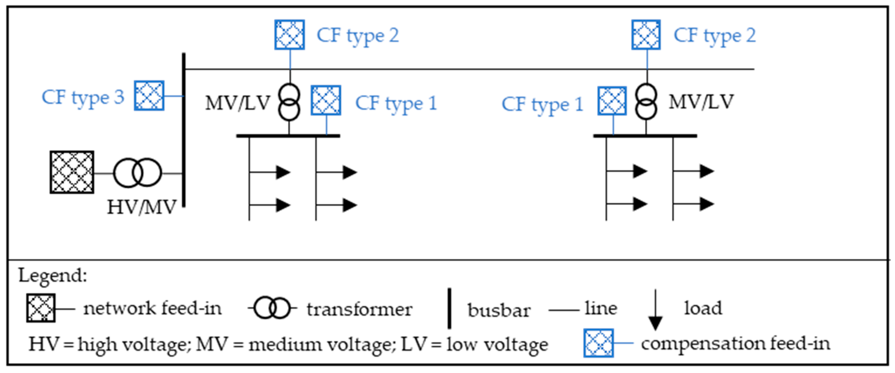
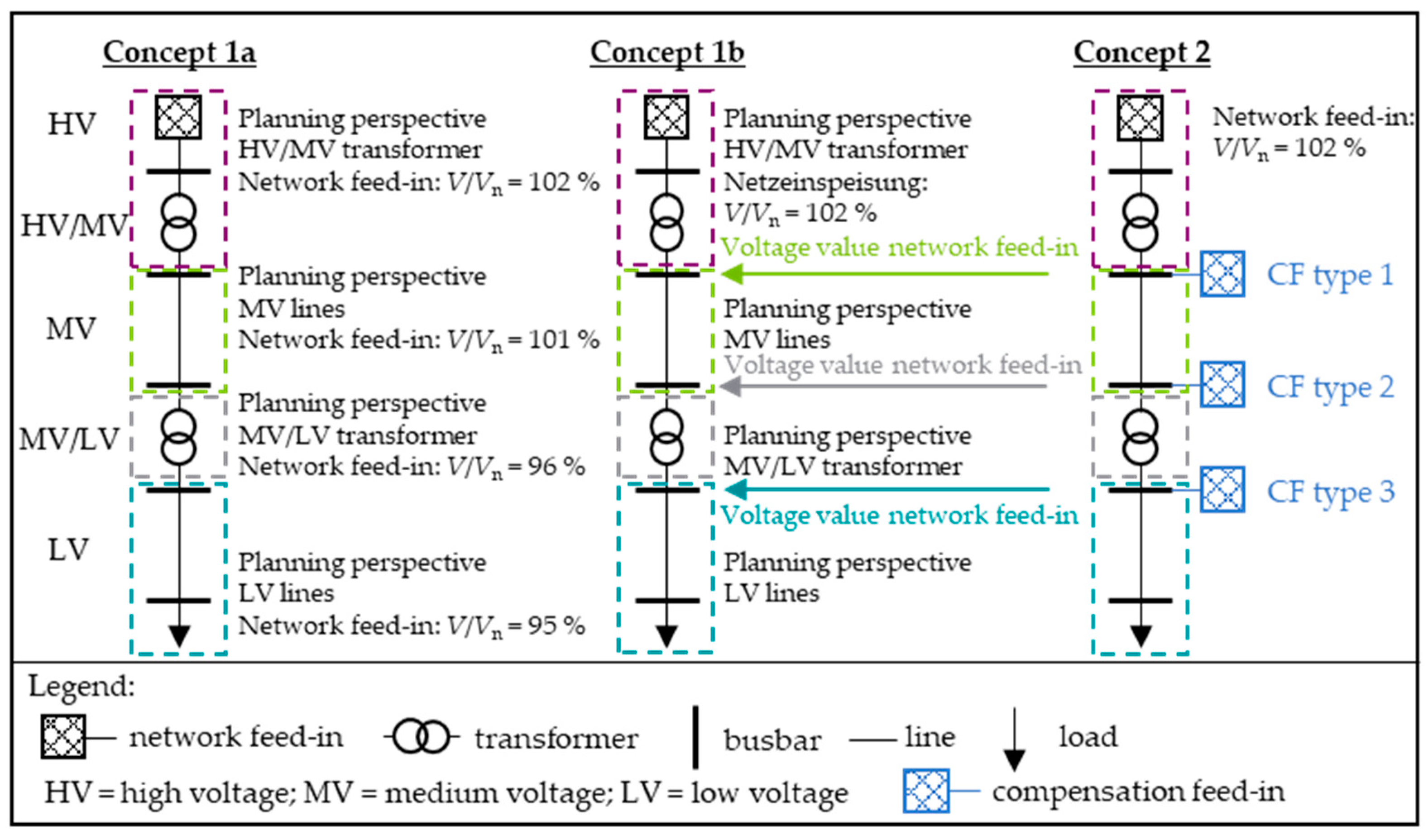
3.2. Concept
- CF type 1 is used for the power compensation between the LV line planning perspective and the MV/LV transformer planning perspective to avoid over-dimensioning of the respective MV/LV transformers. The power values in the respective LV feeder remain unaffected by this. The modelling of the CF type is carried out at the low voltage side of each MV/LV transformer.
- CF type 2 is used for the power compensation between the MV/LV transformer planning perspective and the MV line planning perspective. It is modelled on each high voltage side of the MV/LV transformers. Without this CF, the sum of power per MV feeder is too large, since only the number of loads and DER per MV/LV transformer are taken into account in the SF calculation and not the sum of all loads and DER per MV feeder.
- CF type 3 is used for the power compensation between the MV line planning perspective and the HV/MV transformer planning perspective to avoid over-dimensioning of the respective HV/MV transformers. The modelling of the CF type is carried out at the low voltage side of each HV/MV transformer.
3.3. Modelling Example
4. Application and Results
4.1. Data Set
4.2. Modelling of the Previous Concept (Concept 1)
4.2.1. Concept 1a
| HV/MV transformers: | V/Vn = 102% |
| MV lines: | V/Vn = 101% |
| MV/LV transfomers: | V/Vn = 96% |
| LV lines: | V/Vn = 95% |
4.2.2. Concept 1b
| HV/MV transformers: | V/Vn = 102% |
| MV lines: | Respective voltage values of the low voltage sides of the HV/MV transformers from the planning perspective of the HV/MV transformers |
| MV/LV transfomers: | Respective voltage values of the high voltage sides of the MV/LV transformers from the planning perspective of the MV lines |
| LV lines: | Respective voltage values of the low voltage sides of the MV/LV transformers from the planning perspective of the MV/LV transformers |
4.3. Modelling of the New Concept (Concept 2)
4.4. Overview of the Concepts for the Analyses
4.5. Analysis and Comparison of Concept 2 with Concept 1a
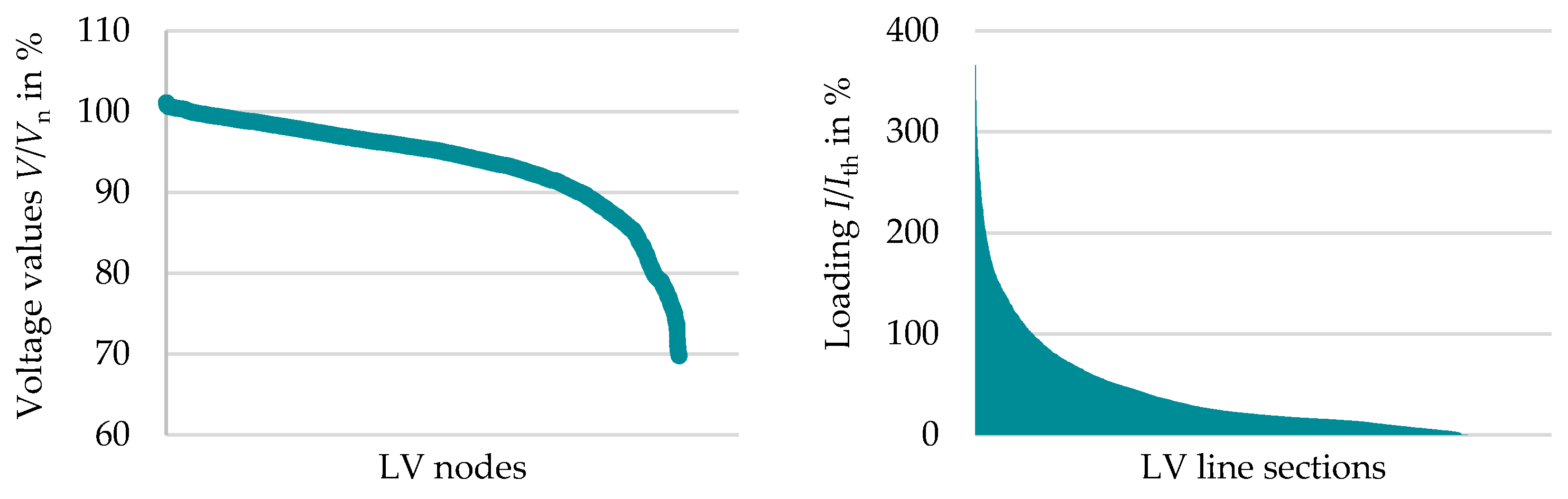
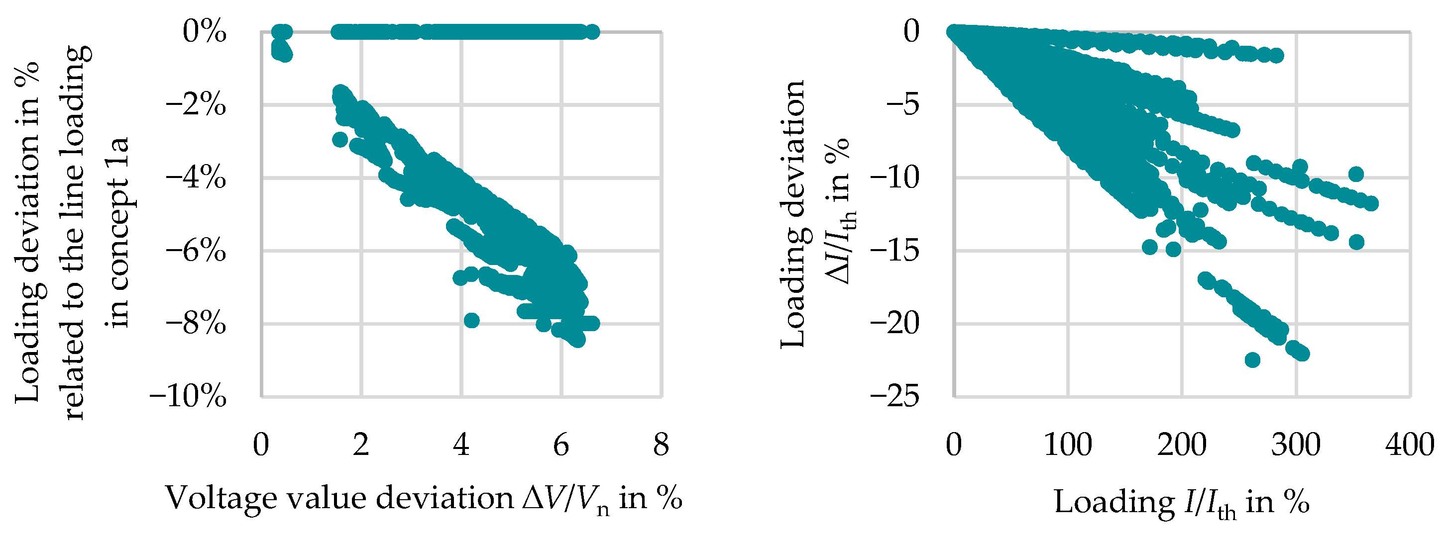
4.5.1. Voltage Band
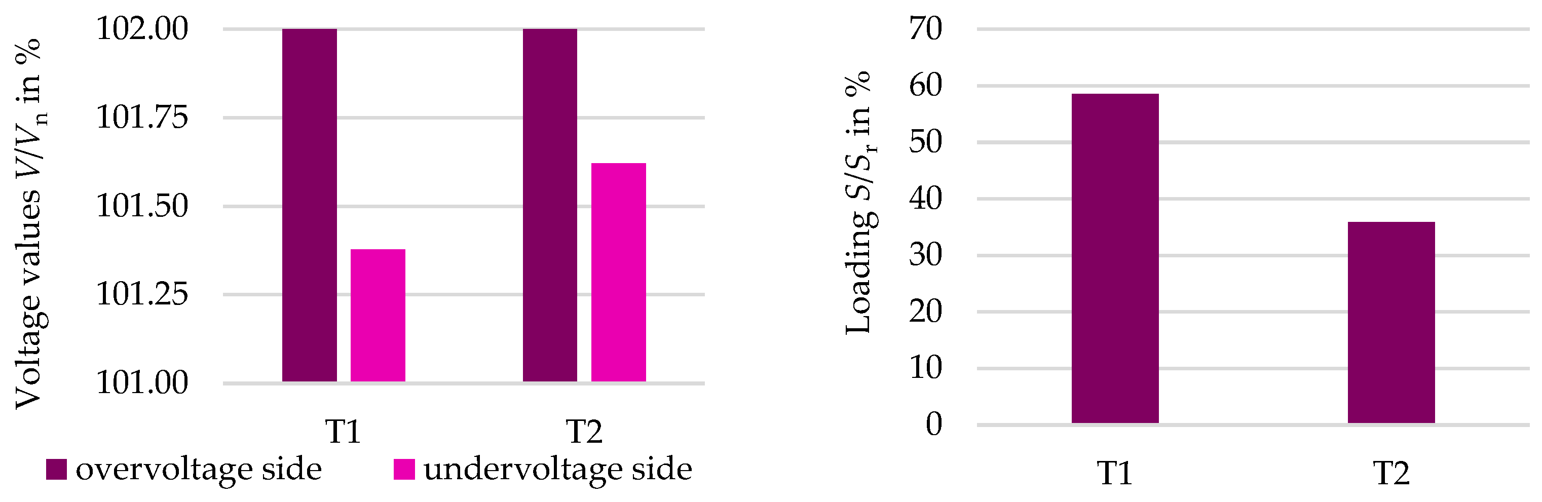
- HV/MV Transformers
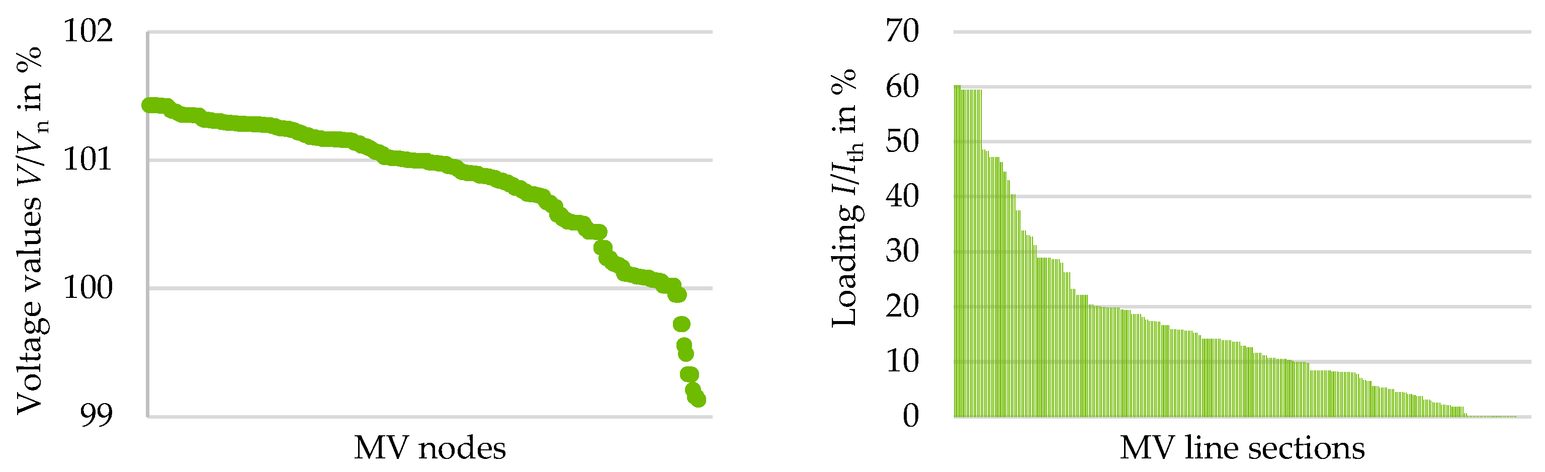
- MV Nodes
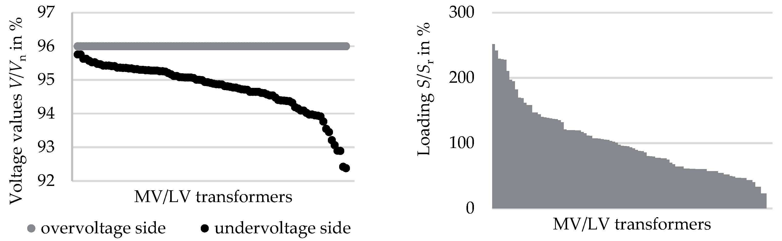
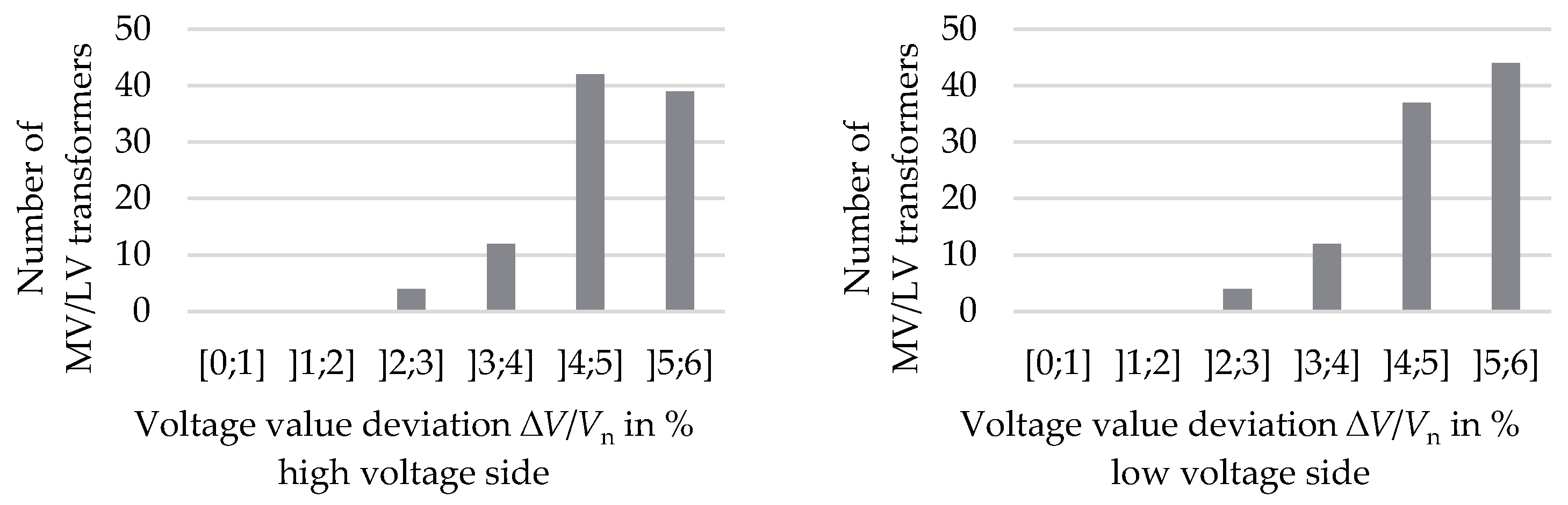
- MV/LV Transformers
- LV Nodes
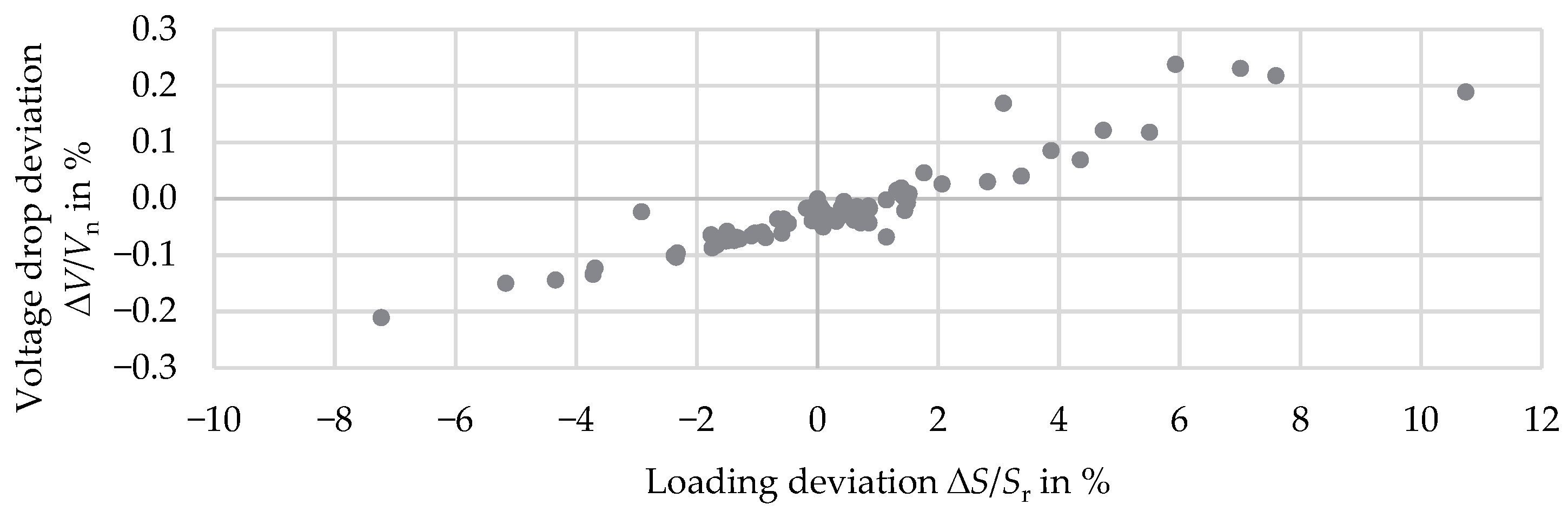
4.5.2. Equipment Loading
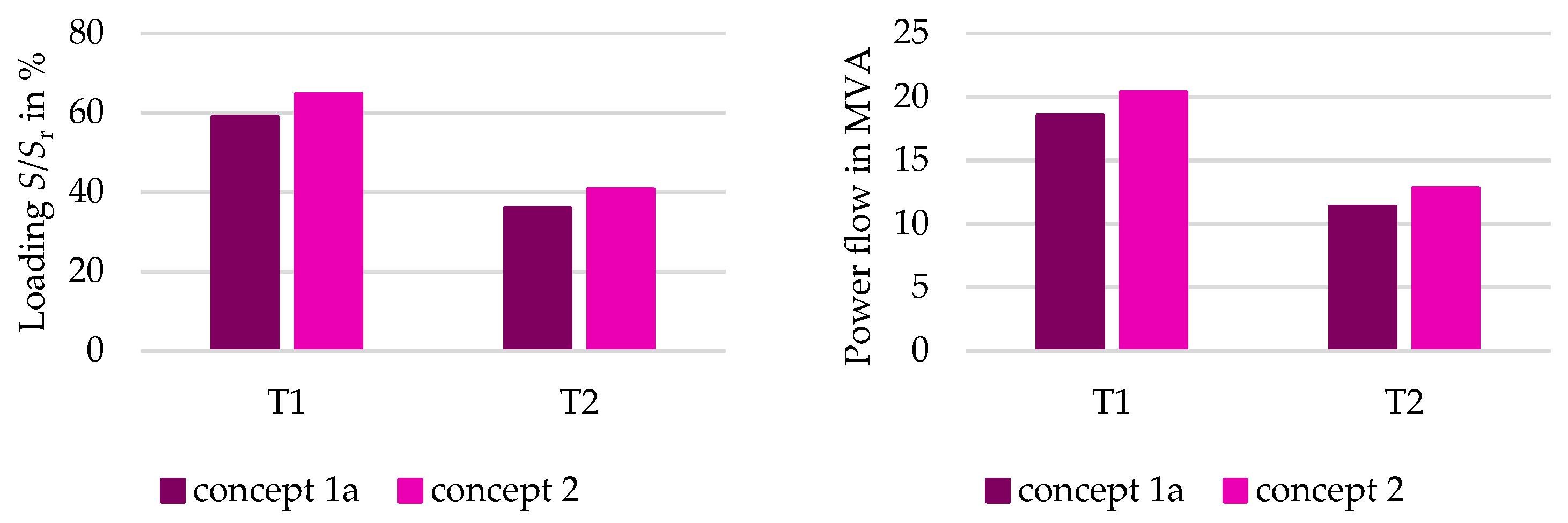
- HV/MV Transformers
- MV Lines
- MV/LV Transformers
- LV Lines
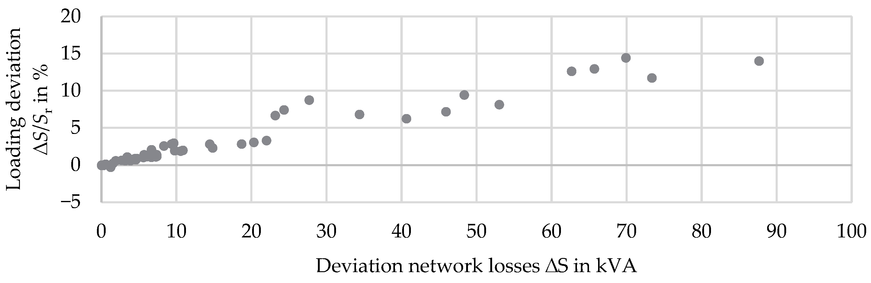
4.5.3. Network Losses
4.5.4. Interim Conclusion
4.6. Analysis and Comparison of Concept 2 with Concept 1b
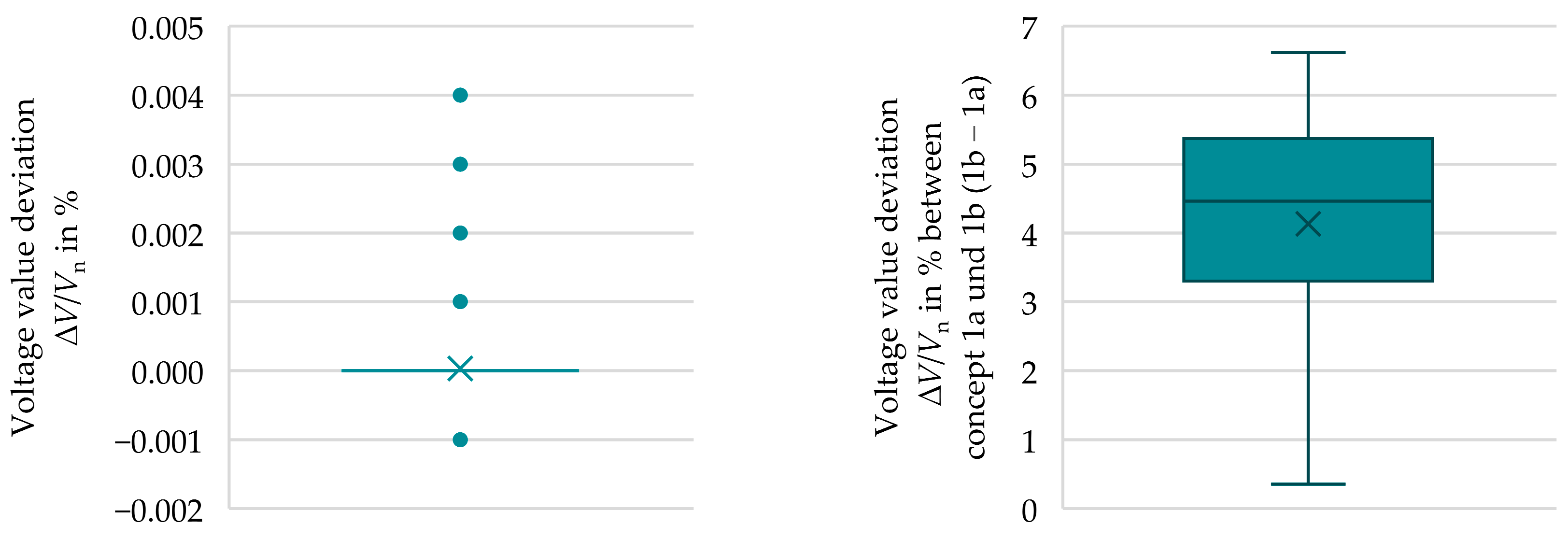
4.6.1. Voltage Band
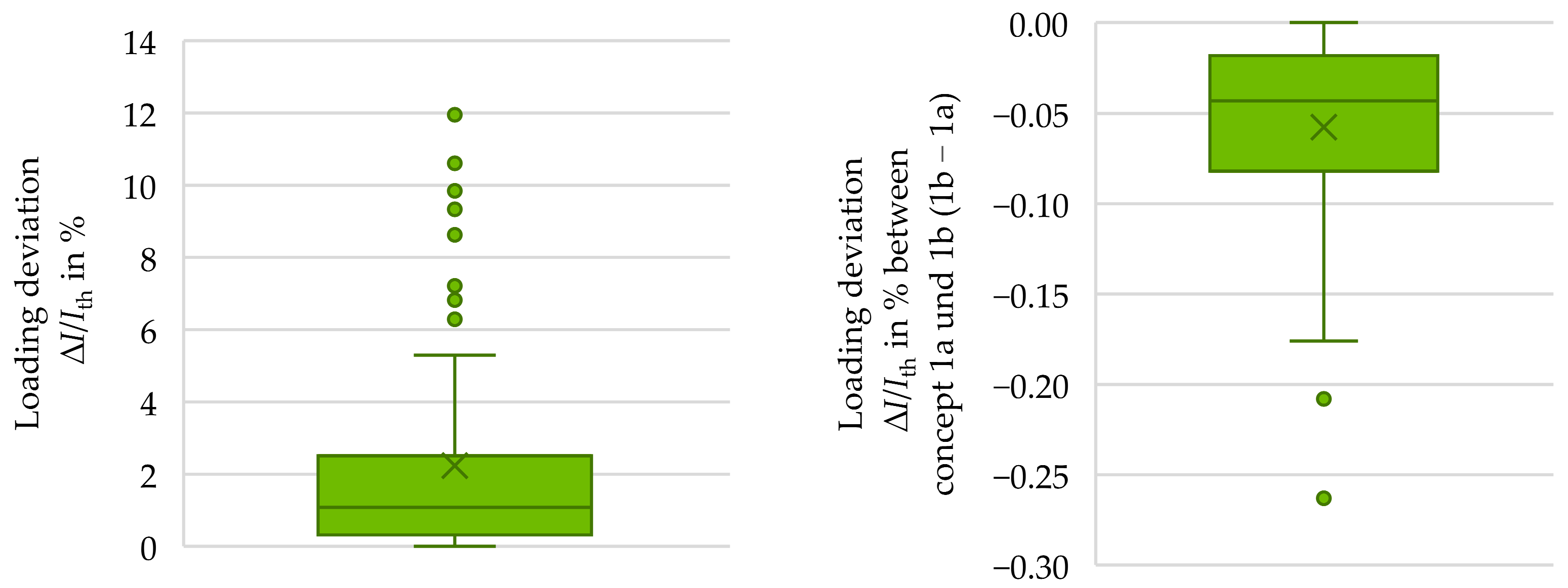
4.6.2. Equipment Loading
4.6.3. Network Losses
4.6.4. Interim Conclusion
4.7. Analysis of the Overplanned Networks
5. Discussion
5.1. Method Reflection
5.2. Influence of the General Conditions
5.3. Fuzziness of Network Modelling
6. Conclusions
Author Contributions
Funding
Data Availability Statement
Conflicts of Interest
References
- United Nations Framework Convention on Climate Change (UNFCCC). Paris Agreement, Conference of the Parties on its Twenty-First Session; UNFCCC: Bonn, Germany, 2015. [Google Scholar]
- Nuss, P.; Günther, J.; Purr, K.; Knoche, G. Rescue—Resource-Efficient Pathways to Greenhouse-Gas-Neutrality; German Environment Agency: Dessau-Roßlau, Germany, 2020.
- International Renewable Energy Agency (IRENA). Rise of Renewables in Cities: Energy Solutions for the Urban Future; International Renewable Energy Agency: Abu Dhabi, United Arab Emirates, 2020; ISBN 978-92-9260-271-0. [Google Scholar]
- German Energy Agency. Integrated Energy Transition—Impulses to Shape the Energy System up to 2050, Report of the Results and Recommended Course of Action; German Energy Agency: Berlin, Germany, 2018. [Google Scholar]
- van Westering, W.; Droste, B.; Hellendoorn, H. Combined Medium Voltage and Low Voltage simulation to accurately determine the location of Voltage Problems in large Networks. In Proceedings of the CIRED 2019 Conference, Madrid, Spain, 3–6 June 2019. [Google Scholar]
- Bolgaryn, R.; Scheidler, A.; Braun, M. Combined Planning of Medium and Low Voltage Networks. In Proceedings of the 13th IEEE PowerTech, Milano, Italy, 23–27 June 2019; ISBN 978-1-5386-4722-6. [Google Scholar]
- Fletcher, R.; Strunz, K. Optimal Distribution System Horizon Planning–Part I: Formulation. Power Systems. IEEE Trans. Power Syst. 2007, 22, 791–799. [Google Scholar] [CrossRef]
- Fletcher, R.; Strunz, K. Optimal Distribution System Horizon Planning–Part II: Application. Power Systems. IEEE Trans. Power Syst. 2007, 22, 862–870. [Google Scholar] [CrossRef]
- Deakin, M.; Greenwood, D.; Walker, S.; Taylor, P. Hybrid European MV–LV Network Models for Smart Distribution Network Modelling. In Proceedings of the IEEE Madrid PowerTech, Madrid, Spain, 28 June–2 June 2021; pp. 1–6. [Google Scholar] [CrossRef]
- Rupolo, D.; Pereira, B.; Contreras, J.; Mantovani, J. Medium- and low-voltage planning of radial electric power distribution systems considering reliability. IET Gener. Transm. Distrib. 2017, 11, 2212–2221. [Google Scholar] [CrossRef]
- Paiva, P.C.; Khodr, H.; Dominguez-Navarro, J.A.; Yusta, J.M.; Urdenata, A.J. Integral planning of primary-secondary distribution systems using mixed integer linear programming. In Proceedings of the IEEE Power Engineering Society General Meeting, 2005, San Francisco, CA, USA, 16 June 2005; Volume 3, p. 2391. [Google Scholar] [CrossRef]
- Navarro, B.B.; Asakil, D.A.H.O.; Navarro, M.M. Medium Voltage to Low Voltage Power Flow Solution Using Modified Backward/Forward Sweep Algorithm. In Proceedings of the IECON 2015—Yokohama 41st Annual Conference of the IEEE Industrial Electronics Society, Yokohama, Japan, 9–12 November 2015; ISBN 978-1-4799-1762-4. [Google Scholar]
- Carter-Brown, C.; Gaunt, C.T. Model for the Apportionment of the Total Voltage Drop in Combined Medium and Low Voltage Distribution Feeders. SAIEE Afr. Res. J. 2006, 97, 57–65. [Google Scholar] [CrossRef]
- Valencia, A.; Hincapie, R.; Gallego, R. Integrated Planning of MV/LV Distribution Systems with DG Using Single Solution-Based Metaheuristics with a Novel Neighborhood Search Method Based on the Zbus Matrix. J. Electr. Comput. Eng. 2022, 2022, 2617125. [Google Scholar] [CrossRef]
- Rupolo, D.; Rodrigues Pereira Junior, B.; Contreras, J.; Mantovani, J. Multiobjective Approach for Medium-and Low-Voltage Planning of Power Distribution Systems Considering Renewable Energy and Robustness. Energies 2020, 13, 2517. [Google Scholar] [CrossRef]
- Rupolo, D.; Mantovani, J.; Rodrigues Pereira Junior, B. Medium-and Low-voltage Planning of Electric Power Distribution Systems with Distributed Generation, Energy Storage Sources, and Electric Vehicles. In Proceedings of the 2019 IEEE Milan PowerTech, Milan, Italy, 23–27 June 2019; pp. 1–5. [Google Scholar] [CrossRef]
- Brunner, H.; Korner, C.; Wieland, T.; Brandl, S.; Ortner, M. Methods and Future Scenarios for Strategic Network Development of full Low and Medium Voltage DSO Supply Areas. In Proceedings of the CIRED 2023 Conference, Rome, Italy, 12–15 June 2023; p. 11066. [Google Scholar]
- Mehigan, L.; Zehir, M.; Cuenca, J.; Şengör, I.; Geaney, C.; Hayes, B. Synergies between Low Carbon Technologies in a Large-Scale MV/LV Distribution System. IEEE Access 2022, 10, 88655–88666. [Google Scholar] [CrossRef]
- DIN EN 50160:2020-11; Voltage Characteristics of Electricity Supplied by Public Electricity Networks. German version EN 50160:2010 + Cor.:2010 + A1:2015 + A2:2019 + A3:2019. DKE Deutsche Kommission Elektrotechnik Elektronik Informationstechnik in DIN und VDE; Beuth Verlag GmbH: Berlin, Germany, 2020.
- German Version EN 50588-1:2017; Medium Power Transformers 50 Hz with Highest Voltage for Equipment not Exceeding 36 kV—Part 1: General Requirements. DKE Deutsche Kommission Elektrotechnik Elektronik Informationstechnik in DIN und VDE; VDE-Verlag GmbH: Berlin, Germany, 2019.
- German Version EN 60076-1:2011; Power Transformers—Part 1: General (IEC 60076-1:2011). DKE Deutsche Kommission Elektrotechnik Elektronik Informationstechnik in DIN und VDE; Beuth Verlag GmbH: Berlin, Germany, 2012.
- DIN VDE 0276-1000:1995-06; Power Cables—Part 1000: Current-Carrying Capacity, General, Conversion Factors. Deutsche Elektrotechnische Kommission im DIN und VDE (DKE); VDE-Verlag GmbH: Berlin, Germany, 1995.
- DIN 18015-1:2020-05; Electrical Installations in Residential Buildings—Part 1: Planning Principles. DIN Deutsches Institut für Normung e. V.; Beuth Verlag GmbH: Berlin, Germany, 2020.
- Wintzek, P.; Ali, S.A.; Riedlinger, T.; Düsterhus, P.; Zdrallek, M. Sensitivity Analysis for Different Calculation Methods of Simultaneity Factors for Charging Infrastructure in Low-Voltage Networks. In Proceedings of the CIRED 2022 Workshop, Porto, Portugal, 2–3 June 2022; p. 1133. [Google Scholar]
- Ali, S.; Wintzek, P.; Zdrallek, M. Development of Demand Factors for Electric Car Charging Points for Varying Charging Powers and Area Types. Electricity 2022, 3, 410–441. [Google Scholar] [CrossRef]
- Wintzek, P.; Ali, S.A.; Kotthaus, K.; Wruk, J.; Zdrallek, M.; Monscheidt, J.; Gemsjäger, B.; Slupinski, A. Application and Evaluation of Load Management Systems in Urban Low-Voltage Network Planning. World Electr. Veh. J. 2021, 12, 91. [Google Scholar] [CrossRef]


| Viewing Area | Number of Loads | P in kW from Planning Perspective LV Lines | P in kW from Planning Perspective MV/LV Transformers | P in kW from Planning Perspective MV Lines | P in kW from Planning Perspective HV/MV Transformer |
|---|---|---|---|---|---|
| 1 load | 1 | 22.71 | 20.15 | 19.14 | 19.14 |
| 1 LV feeder | 2 | 45.42 | 40.30 | 38.28 | 38.28 |
| 1 MV/LV transformer | 4 | 90.84 | 80.60 | 76.56 | 76.56 |
| 1 MV feeder | 8 | 181.68 | 161.20 | 153.12 | 153.12 |
| 1 HV/MV transformer | 8 | 181.68 | 161.20 | 153.12 | 153.12 |
| Parameter | Value | Unit |
|---|---|---|
| Power rating of the HV/MV transformers | 31.5 | MVA |
| MV line length | 56.4 | km |
| MV feeders | 14 | pieces |
| Distribution stations | 53 | pieces |
| Customer stations | 26 | pieces |
| LV line length | 135 | km |
| House connections | 3286 | pieces |
| Metering points | 13,893 | pieces |
| Private charging points | 5303 | pieces |
| Public charging points | 501 | pieces |
| Electric heat pumps | 1014 | pieces |
| Equipment | Parameter | Concept 2 | |
|---|---|---|---|
| Effect | Justification | ||
| HV/MV transformers | Voltage values | Lower | Higher voltage drop |
| Voltage drop | Higher | Higher network losses | |
| Loading | Higher | Higher network losses | |
| Network losses | Higher | Loading of the equipment from their respective planning perspective, additional modelling of LV lines | |
| MV nodes/ MV lines | Voltage values | Higher | Voltage band of the HV/MV transformer network level not fully utilized |
| Lower | Higher network losses | ||
| Loading | Higher | Higher network losses | |
| Network losses | Higher | Loading of the equipment from their respective planning perspective, additional modelling of LV lines | |
| MV/LV transformers (DT) | Voltage values | Higher | Voltage band of the overlying network levels is not fully utilized |
| Voltage drop | Higher Lower | Higher network losses Higher voltage values | |
| Loading | Higher Lower | Higher network losses Higher voltage values | |
| Network losses | Higher | LV line loading from their respective planning perspective | |
| MV/LV transformers (CT) | Voltage values | Higher | Voltage band of the overlying network levels is not fully utilized |
| Voltage drop | Lower | Higher voltage values | |
| Loading | Lower | Higher voltage values | |
| Network losses | Lower | Higher voltage values | |
| LV nodes/ LV lines | Voltage values | Higher | Voltage band of the overlying network levels is not fully utilized |
| Loading | Lower | Higher voltage values | |
| Network losses | Lower | Higher voltage values | |
| Equipment | Parameter | Concept 2 | |
|---|---|---|---|
| Effect | Justification | ||
| HV/MV transformers | Voltage values | Lower | Higher voltage drop |
| Voltage drop | Higher | Higher network losses | |
| Loading | Higher | Higher network losses | |
| Network losses | Higher | Loading of the equipment from their respective planning perspective, additional modelling of LV lines | |
| MV nodes/ MV lines | Voltage values | Lower | Higher network losses |
| Loading | Higher | Higher network losses | |
| Network losses | Higher | Loading of the equipment from their respective planning perspective, additional modelling of LV lines | |
| MV/LV transformers (DT) | Voltage values | Lower | Higher voltage drops |
| Voltage drop | Higher | Higher network losses | |
| Loading | Higher | Higher network losses | |
| Network losses | Higher | LV line loading from their respective planning perspective | |
| MV/LV transformers (CT) | Voltage values | Equal | Equal network losses |
| Voltage drop | Equal | Equal network losses | |
| Loading | Equal | Equal network losses | |
| Network losses | Equal | No network losses through underlying network levels | |
| LV nodes/ LV lines | Voltage values | Equal | Equal network losses |
| Loading | Equal | Equal network losses | |
| Network losses | Equal | ||
| Equipment | Parameter | Concept 2 | |
|---|---|---|---|
| Effect | Justification | ||
| HV/MV transformers | Voltage values | Lower | Higher voltage drop |
| Voltage drop | Higher | Higher network losses | |
| Loading | Higher | Higher network losses | |
| Network losses | Higher | Loading of the equipment from their respective planning perspective, additional modelling of LV lines | |
| MV nodes/ MV lines | Voltage values | Lower | Higher network losses |
| Loading | Higher | Higher network losses | |
| Network losses | Higher | Loading of the equipment from their respective planning perspective, additional modelling of LV lines | |
| MV/LV transformers (DT) | Voltage values | Lower | Higher voltage drop |
| Voltage drop | Higher | Higher network losses | |
| Loading | Higher | Higher network losses | |
| Network losses | Higher | LV line loading from their respective planning perspective | |
| MV/LV transformers (CT) | Voltage values | Equal | Equal network losses |
| Voltage drop | Equal | Equal network losses | |
| Loading | Equal | Equal network losses | |
| Network losses | Equal | No network losses through underlying network levels | |
| LV nodes/ LV lines | Voltage values | Equal | Equal network losses |
| Loading | Equal | Equal network losses | |
| Network losses | Equal | ||
Disclaimer/Publisher’s Note: The statements, opinions and data contained in all publications are solely those of the individual author(s) and contributor(s) and not of MDPI and/or the editor(s). MDPI and/or the editor(s) disclaim responsibility for any injury to people or property resulting from any ideas, methods, instructions or products referred to in the content. |
© 2024 by the authors. Licensee MDPI, Basel, Switzerland. This article is an open access article distributed under the terms and conditions of the Creative Commons Attribution (CC BY) license (https://creativecommons.org/licenses/by/4.0/).
Share and Cite
Riedlinger, T.; Wintzek, P.; Zdrallek, M. Development of a New Modelling Concept for Power Flow Calculations across Voltage Levels. Electricity 2024, 5, 174-210. https://doi.org/10.3390/electricity5020010
Riedlinger T, Wintzek P, Zdrallek M. Development of a New Modelling Concept for Power Flow Calculations across Voltage Levels. Electricity. 2024; 5(2):174-210. https://doi.org/10.3390/electricity5020010
Chicago/Turabian StyleRiedlinger, Tobias, Patrick Wintzek, and Markus Zdrallek. 2024. "Development of a New Modelling Concept for Power Flow Calculations across Voltage Levels" Electricity 5, no. 2: 174-210. https://doi.org/10.3390/electricity5020010