Disaggregating Longer-Term Trends from Seasonal Variations in Measured PV System Performance

Abstract

Photovoltaic (PV) systems are widely adopted for renewable energy generation, but their performance is influenced by complex interactions between longer-term trends and seasonal variations. This study aims to remove these factors and provide valuable insights for optimising PV system operation. We employ comprehensive datasets of measured PV system performance over five years, focusing on identifying the distinct contributions of longer-term trends and seasonal effects. To achieve this, we develop a novel analytical framework that combines time series and statistical analytical techniques. By applying this framework to the extensive performance data, we successfully break down the overall PV system output into its constituent components, allowing us to find out the impact of the system degradation, maintenance, and weather variations from the inherent seasonal patterns. Our results reveal significant trends in PV system performance, indicating the need for proactive maintenance strategies to mitigate degradation effects. Moreover, we quantify the impact of changing weather patterns and provide recommendations for optimising the system’s efficiency based on seasonally varying conditions. Hence, this study not only advances our understanding of the intricate variations within PV system performance but also provides practical guidance for enhancing the sustainability and effectiveness of solar energy utilisation in both residential and commercial settings.

1. Introduction

Disaggregating longer-term trends from seasonal variations in measured PV system performance is an important aspect of understanding the performance of solar photovoltaic (PV) systems [1,2,3]. Seasonal variations in the performance ratios for PV systems can be obscured by diurnal and seasonal changes, making it difficult to determine long-term performance degradation from transient performance changes [2]. The performance ratio (PR) is a commonly used metric to measure solar PV plant performance. Still, it is insufficient to use as the basis for a performance guarantee when precise confidence intervals are required due to the large seasonal variation in PR [3]. To reduce seasonal variations of the PR due to the temperature dependency of the used PV cell, the PR may be corrected for temperature [2].

Seasonal variations can have a significant effect on the performance of solar PV systems [3,4,5,6]. For instance, the amount of sunlight hitting the solar panels varies throughout the year, with shorter days and less direct sunlight in the winter [5]. This can result in decreased energy output during the winter months, which can be compensated for by increasing the size of the solar array or by storing excess energy in batteries [5,6]. However, the temperature can affect the performance of PV systems, with the PR being corrected for temperature to reduce seasonal variations [3].

PV systems are subject to a multitude of factors that influence their output, such as solar irradiance variations, temperature effects, shading, and system degradation [1,2,3]. While seasonal variations can be attributed to changes in solar position and meteorological conditions, longer-term trends may arise from factors such as module ageing, performance degradation, and gradual system efficiency disimprovement [1,2,3]. Identifying and quantifying these trends is essential for accurate performance evaluation and predictive maintenance. Photovoltaic (PV) modules that convert solar energy into electrical energy [1] gradually degrade over time [7] giving reduced output power manifest in a lower performance ratio [8]. The module degradation rate depends on the specification and manufacture of PV modules as well as operational ambient temperatures and their variation, relative humidity, intensity and spectrum of incident solar radiation, wind speed, and extent of exposure to rain, snow, and dust [1]. Even for nominally identical systems, degradation rates measured in one location cannot thus be assumed to apply in another location [8,9]. Distinguishing between underlying multi-annual trends and periodic seasonal variations in measured PV system outputs is a prerequisite for identifying longer-term performance degradation. One way to implement this is to “correct” the PV PR for either ambient or module temperature [3,10]. Correlations between power loss in a PV system with cell temperature, irradiance, temperature variations, and shading have been found in previous studies [11]. For instance, the main factors that impact power loss in a PV system are: (i) Cell Temperature: The temperature of the solar cells can significantly affect their efficiency. As cell temperature increases, the efficiency of the cells tends to decrease due to the negative temperature coefficient of most PV materials, which causes their output voltage and current to decrease with increasing temperature. The correlation between cell temperature and power loss is usually negative [12,13]. (ii) Irradiance: Irradiance refers to the amount of solar energy that reaches the solar cells. Higher irradiance levels generally lead to higher output power from the PV system. The correlation between irradiance and output power is positive [14,15]. (iii) Temperature Variations: Temperature variations can impact the performance of a PV system, including fluctuations in ambient temperature throughout the day [13]. Temperature changes can influence the efficiency of the system due to changes in cell temperature and, consequently, cell efficiency [13]. The correlation between temperature variations and power loss can be both positive and negative, depending on the specific conditions [13]. (iv) Shading: Shading is a critical factor that can cause power loss in a PV system. When a portion of the PV array is shaded, it can create “hot spots” and reduce the overall system efficiency [14,15]. This is because the shaded cells can become reverse-biased, leading to power losses, and potentially damaging the shaded cells. The correlation between shading and power loss is typically negative [14,15].

This paper aims to develop methods to separate the long-term trends from seasonal variations in the measured PV system performance [16]. This has been a topic of previous research. For example, (i) Lindig et al. [2] focus on best practices for performance loss rate (PLR) computations, and the challenges and opportunities associated with it, but it does not directly address the methods for disaggregating longer-term trends from seasonal variations in measured PV system performance. To address this, this study adds two more accurate and reliable methods for calculating PLR (such as relative PLR (PLR_rel) and absolute PLR (PLR_abs)). (ii) In Dierauf et al.’s [3] study, traditional PR computation neglects array temperature, which typically results in seasonal variation. This seasonal variation makes the PR metric insufficient to use as the basis for a performance guarantee when precise confidence intervals are required. To reduce the seasonality effects, this study carried out the annual average cell temperature of the three locations (Harlequins, Newry, and Warrrenpoint). Hence, the traditional PR “uncorrected PR” now normalises with the annual average cell temperature to become normalised PR “temperature-corrected PR”. This resulting weather-corrected PR or “temperature-corrected PR” gives more consistent results throughout the year, enabling its use as a metric for performance guarantees.

2. Solar PV Performance Monitoring

Solar PV performance monitoring is the process of observing and recording the parameters from the solar PV power plant in real-time [17]. The development of an advanced monitoring method is crucial for the efficient and reliable operation of solar PV systems [17]. The primary purposes of monitoring PV systems encompass measuring energy output, evaluating the performance of the PV system, and promptly detecting any design faults or operational problems [18]. In the case of large PV systems, analytical monitoring is employed to proactively mitigate economic losses arising from operational challenges [18]. The performance analysis of grid-connected PV systems involves comparing and presenting the operational results of such systems [19]. This includes investigating the performance of PV systems based on different module technologies [20]. The analytical monitoring of grid-connected PV systems involves measuring and analysing various parameters such as irradiation sensors, energy generation measurements, and performance indicators [18]. This can also involve monitoring the performance of PV systems before and after the application of a set of procedures for performance analysis [21]. Hence, good practices for monitoring and performance analysis of grid-connected PV systems include [21]: (i) Establishing a standard method for monitoring the performance of long-term PV systems in buildings. (ii) Creating a set of good practices and systematic analysis for the monitoring of PV systems, considering performance indicators, as well as temperature, cable, and energy conversion losses. (iii) Developing a set of procedures for performance analysis of small grid-connected PV systems, classified in terms of project, installation site, electrical installation, protection, safety, and maintenance.

For instance, an examination of failures in grid-connected residential PV systems with capacities ranging from 1 to 5 kW_p, installed in Germany during the 1990s [22], revealed that, on average, a failure occurred approximately every 4.5 years per installation. Among these failures, inverters accounted for 63%, PV modules for 15%, and other system components for 22% of the total failures [18]. A failure detection routine (FDR) was introduced to compare the monitored energy yield with the simulated yield for a given period [23,24]. The FDR used comprised three core components: (i) the failure detection system, (ii) the failure profiling method, and (iii) the footprint method. When a substantial disparity exists between the monitored and simulated energy yields, the FDR identifies a potential failure. It further characterises the energy loss pattern by creating a profile of the actual failure and contrasting it with pre-defined profiles of frequently occurring failures. Based on the correlation between the actual failure profile and these pre-defined profiles, the FDR assesses the likelihood of various failure scenarios. The footprint method aids in the analysis of patterns across three distinct domains: (i) normalised monitored power, time (hour of the day), and sun elevation. This method was developed through the examination of common system faults using data from well-monitored PV installations within the German 1000-roofs programme. Initial findings, as reported [23], indicate that the methodology is effective in identifying failures that are unequivocally implausible. However, further refinement is required. Field tests, as discussed [25], have demonstrated that the time needed to detect a failure using the PVSAT-2 routine [26], which employs the FDR methodology, can vary considerably, ranging from as little as one day to several months. This variability is primarily influenced by factors such as weather conditions, the scale of the failure, and its duration.

2.1. Seasonal Variations in PV Performance

To enhance the reliability and durability of PV systems, PV manufacturers should conduct rigorous stress tests to assess their optimised performance. This is particularly crucial due to the impact of temperature-induced seasonal variations [27]. For instance, Jiaying et al. [28] examined three different PV module technologies: monocrystalline silicon (m-Si), single junction amorphous silicon (a-Si), and micromorph silicon thin-film modules. The results of their correlation analysis indicate that temperature plays a pivotal role in seasonal performance variations. Monocrystalline silicon exhibits the strongest correlation with both temperature and irradiance. In contrast, single junction a-Si modules display lower sensitivity to temperature variations, while micromorph silicon modules demonstrate the weakest correlation with these two variables.

Installed PV modules in real-world conditions have been shown to exhibit seasonal performance fluctuations [29]. These variations stem from two main factors [28]: (i) Temperature Variation Between Seasons: The difference in temperature between summer and winter seasons is a key influencer. PV modules with a more negative temperature coefficient of maximum power tend to perform better in winter than in summer. Furthermore, thin-film and a-Si modules subjected to thermal annealing processes recover from light-induced defects (LID), leading to improved performance during the summer. (ii) Spectral Variability Due to Sun Position: Variations in the sun’s position throughout the year affect the spectral characteristics of sunlight and consequently impact PV system performance. For example, in PV materials with a wider band gap, such as a-Si, spectral variability plays a role in module performance. These modules tend to perform better in the summer when exposed to a blue-rich spectrum of light but exhibit reduced performance in the winter under a red-rich spectrum [30]. The output of PV modules fluctuates in response to incident solar irradiance and module temperature, making the energy output of a system contingent on prevailing weather conditions [4,31]. An increase in PV cell temperatures can result in reduced output and efficiency [27]. However, the performance of a solar photovoltaic system is dependent on many site factors such as latitude, season, cloudiness, and air pollution [32]. This means that seasonal variations have a significant impact on the performance of solar photovoltaic installations [32]. Thus, the following are some of the factors that affect the seasonal variations in PV performance [4,32]: (i) Sunshine Period: The trend of the monthly average daily sunshine period affects the performance of PV systems. During July and August, the sunshine period was lower due to the southwest monsoon over the Indian subcontinent, which was reflected in the yield of the PV system. (ii) Spectral Variations: The spectral variations due to seasonal changes in the incident spectrum also affect the performance of PV systems. A study conducted in India showed that PV technologies which have broad spectral bands give higher utilisation factor (UF) values compared to technologies that have narrow spectral bands. The study also found that seasonal spectral variations have a significant impact on the performance of different PV technologies. (iii) Seasonality: Seasonality is the variation in solar generation due to seasonal changes in the angle of the sun. In most areas of the United States, solar panels yield the highest generation in the summer months, followed by fall and spring. This is because the days are longer, and the sun is higher in the sky during these months. In contrast, solar panels generate less power in the winter months when the days are short, and the sun is low. Therefore, to account for seasonal variations in PV performance, it is essential to consider the factors mentioned above during the design and installation of PV systems. The seasonal variations in PV performance should also be considered when estimating the solar offset and monthly savings of a solar energy system [32].

2.2. Performance Ratio Corrected for Temperature (PR_Corr)

The performance ratio (PR) in solar PV installations normalises system output relative to the installed capacity and the available solar irradiance at the installation site. PR facilitates the comparison of system performance across varying installed capacities and geographical locations [33]. The weather-uncorrected performance ratio is determined using Equation (1) [33]. To account for temperature effects, PR can be adjusted by incorporating a temperature correction, resulting in a “temperature-corrected” PR_Corr [3,33], as shown in Equation (2). This is because, in 2021, the average cell temperatures across the three locations (Harlequins, Newry, and Warrenpoint) studied were significantly increased compared to the years 2017 through 2020.

Table 1. Specifications and locations of the monitored arrays.

	PV Array Location
	Harlequins	Newry	Warrenpoint
Tilt and Azimuth Angles	Azimuth: −162°, Tilt: 12° for PV array 1 Azimuth: 12°, Tilt: 12° for PV array 2	Azimuth: −31°, Tilt: 6° for PV array 1 Azimuth: 149°, Tilt: 6° for PV array 2	Azimuth: −125°, Tilt: 7° for PV array 1 Azimuth: 55°, Tilt: 7° for PV array 2
Total PV Area	312.36 m2	311.04 m2	268.8 m2
Solar Cell Technology	Polycrystalline silicon (p-Si)	-	-
PV Module Manufacturer	Renesola	-	-
Module Rating	260 Wp at STC	-	-
Number of Modules	192	-	-
Installation Type	Rooftop	-	-
PV Capacity	49.92 kWp at STC	-	-
Module type (s)	Renesola-JC260M-24/Bbv (260 W)	-	-
Inverter	Sunny TriPower	-	-
Inverter Capacity [AC]	2 × 20 kW	-	-

shows the specifications and locations of the three monitored arrays. This temperature increase was attributed to an intense heatwave during that year, as demonstrated in

Table 2. Average annual PV cell temperatures for Harlequins, Newry, and Warrenpoint.

Year	Harlequins	Newry	Warrenpoint
	Average cell Temperature, Tcell_avg (°C)	Average cell Temperature, Tcell_avg (°C)	Average cell Temperature, Tcell_avg (°C)
2017	37.87	37.21	37.09
2018	38.37	38.14	37.70
2019	39.95	37.14	36.09
2020	38.06	36.50	36.79
2021	39.98	39.76	39.68

.

Therefore, the novelty of this study is based on the following [34]: (i) The degradation rates observed in the three arrays, namely Harlequins, Newry, and Warrenpoint, are linear. This linearity arises because all the modules under investigation are operating within the stable region of their respective “bathtub” failure rate curves. (ii) The primary parameters governing seasonal behaviour in this context are cell temperature and solar irradiance. This is because key performance indicators of PV systems, such as system efficiency and power output, exhibit linear dependencies on cell temperature and irradiance. When solar irradiance surpasses 500 W/m², it leads to an increase in cell temperature, subsequently causing a reduction in both the efficiency and power output of the PV system [35,36]. Consequently, an increase in cell temperature results in decreased system efficiency and power output, while a decrease in cell temperature leads to an enhancement in both efficiency and power output. (iii) Long-term performance assessment of PV systems can be challenging due to the fluctuating environmental conditions that occur on a daily and seasonal basis. To mitigate the impact of these variable conditions, the weather-uncorrected performance ratios (PR_Uncorr) were adjusted through the utilisation of the annual average cell temperature (T_{Cell_avg}) recorded in Table 2. The incorporation of this temperature correction served to reduce the seasonal variabilities in the performance ratio, thus enabling the separation of longer-term trends from the influence of seasonal variabilities.

3. Materials and Methods

The study aims to address the challenge of disaggregating longer-term trends from seasonal variations in measured PV system performance. To achieve this, a comprehensive approach that integrates statistical and time-series analyses is employed. The following sections outline the materials used and the methods applied in this study: (i) Data Collection and Pre-processing: Five years of historical data from an operational PV system, including solar irradiance, module temperature, and output power measurements, are collected. The data are obtained from a diverse range of geographical locations (Harlequins, Newry, and Warrenpoint in Northern Ireland) and periods to ensure the robustness of the analysis. Data pre-processing used in this study involves outlier removal, missing value imputation, and synchronisation of time-series data [37]. (ii) Time-Series Decomposition: Classical time-series decomposition techniques, such as the seasonal decomposition of time-series (STL), are applied to disaggregate the underlying components of the PV system’s performance [38]. (iii) Wavelet Analysis: Wavelet transform is employed to analyse the time–frequency representation of the PV system’s output power. By decomposing the time series into different frequency components, wavelet analysis helps identify both short-term fluctuations and underlying long-term trends [39]. Hence, three roof-mounted grid-connected PV arrays located in Northern Ireland were monitored for five years. These arrays are designated (after their locations) “Harlequins”, “Newry”, and “Warrenpoint”. The specifications and locations of the three arrays are provided in Table 1. In-plane irradiance (G_POA), AC output power (P_AC), and cell temperature (T_cell) were measured at fifteen-minute intervals using pyranometers, AC power meters, and thermocouples. The continuous monitoring of the PV system performance parameters (such as electrical output, efficiency, and temperature) across the three locations was conducted using data logging equipment. From the data collected, performance fluctuations were observed as a result of seasonal variations. To disaggregate longer-term trends from seasonal variations in measured PV system performance located in Harlequins, Newry, and Warrenpoint, the weather-uncorrected performance ratios as seen in Equation (1) of Section 4 were converted to temperature-corrected performance ratios (i.e., weather-corrected performance ratios) using the average annual cell temperatures (T_{cell_avg}) shown in Table 2 and Equation (3). The azimuth and tilt angles of the PV arrays are shown in the first row of Table 1.

4. Results

4.1. Data Collection and Preprocessing

PV systems used in this study are typically equipped with sensors and monitoring equipment that record various performance metrics such as solar irradiance, temperature, voltage, current, and power output. Data were reliably and consistently collected from these sensors which spread across Harlequins, Newry, and Warrenpoint at fifteen-minute intervals. To clean up the data, missing data were handled through data interpolation. Outliers were removed to avoid distortion in the data analysis [37].

4.2. Time Series

To investigate long-term degradation, relative performance loss rates (PLR_rel), absolute performance loss rates (PLR_abs), and nonlinear trends over five years were fitted to simple best-fit linear lines. Uncorrected and module temperature-corrected annual monthly relative and absolute performance loss rates from Harlequins, Newry, and Warrenpoint arrays from 2017 to 2021, the gradient (β₁) and the y-intercept (β_o) of each year across the three arrays were found using the time-series (Y_t{XE “Yt:Linear regression model”}) linear regression model, as shown in Equation (12) [40]. This separates longer-term trends from seasonal variations [39].

4.3. Wavelet Analysis

By utilising temperature-corrected performance ratios, it becomes possible to discern long-term performance degradation trends with a high degree of confidence after just six months for one PV array and within three years for the other two arrays. If a lower level of statistical confidence in these trends is acceptable, it is still feasible to identify long-term degradation rates within one year of operation for all PV arrays under investigation. These findings hold significant implications, as they suggest that relatively brief outdoor PV performance monitoring can reliably serve as a means to estimate long-term degradation and/or to calibrate the typically conducted accelerated testing processes. For instance, data exhibiting a high coefficient of determination (R²) concerning a linear trend suggests that the trend can be extrapolated with reliability. In this context, R² values of 0.810 and 0.999 are selected to signify a robust correlation with the dataset. Figure 1 and Figure 2 illustrate the enhancements in coefficients of determination (R²) for PR, computed over varying cumulative time intervals. Temperature-corrected PR values achieve R² coefficients of determination of 0.810 and 0.999 within cumulative degradation trend evaluation periods ranging from 6 months (for the Warrenpoint PV array and system) to approximately 3 years for the Harlequins and Newry PV arrays and systems. In contrast, “weather-uncorrected” PR values necessitate lengthier cumulative evaluation periods, approximately 4 years, to attain R² coefficients of determinations of 0.810 and 0.999 for their long-term degradation trends. These findings highlight that temperature-corrected PR values enable the earlier detection of long-term degradation trends.

4.4. Performance Ratio

The photovoltaic system performance ratio (PR) compares the actual and theoretical energy yields of the PV systems [41]. By normalising system performance to its installed power and available solar radiation at the installation site, the PR enables comparison of the performances of dissimilar PV systems in different geographic locations [4,38,42,43]. PR can be calculated on a yearly, monthly, or daily basis. The performance ratio, PR_uncorr, is calculated using Equation (1) [33]:

$${\mathrm{P}\mathrm{R}}_{\mathrm{u}\mathrm{n}\mathrm{c}\mathrm{o}}=\frac{{\sum \mathrm{P}}_{\mathrm{A}\mathrm{C}\_\mathrm{t}}}{\sum _{\mathrm{t}}{[\mathrm{P}}_{\mathrm{S}\mathrm{T}\mathrm{C}}(\frac{{\mathrm{G}}_{\mathrm{P}\mathrm{O}\mathrm{A}}}{{\mathrm{G}}_{\mathrm{S}\mathrm{T}\mathrm{C}}})]}\times 100\mathrm{\%},$$

(1)

where P_AC{XE “P_AC:Measured AC electrical generation”_}: measured AC electrical generation (W).

P_STC: installed PV module capacity (in the instance of the PV arrays examined 49,920 W_p).

G_POA: measured plane of array irradiance (W/m²).

t{XE “t:data collection period”}: data collection period.

G_STC{XE “G_STC:Irradiance at standard test conditions”_}: irradiance at standard test conditions (1000 W/m²).

Introducing a correction based on cell temperature to calculate PR_corr gives [35]

$${\mathrm{P}\mathrm{R}}_{\mathrm{c}\mathrm{o}\mathrm{r}\mathrm{r}}=\frac{{\sum \mathrm{P}}_{\mathrm{A}\mathrm{C}\_\mathrm{t}}}{\sum _{\mathrm{t}}{[\mathrm{P}}_{\mathrm{S}\mathrm{T}\mathrm{C}}(\frac{{\mathrm{G}}_{\mathrm{P}\mathrm{O}\mathrm{A}}}{{\mathrm{G}}_{\mathrm{S}\mathrm{T}\mathrm{C}}})(1-\frac{\mathsf{\delta }}{100}\left({\mathrm{T}}_{\mathrm{c}\mathrm{e}\mathrm{l}\mathrm{l}\_\mathrm{a}\mathrm{v}\mathrm{g}-{\mathrm{T}}_{\mathrm{c}\mathrm{e}\mathrm{l}\mathrm{l}}}\right))]},$$

(2)

where T_cell{XE “T_{cell_avg:} Average annual solar cell temperature”_{}_avg}: average annual PV cell temperature (°C).

T_cell: instantaneous PV cell temperature (°C).

$\delta :$ tmperature coefficient of PV array power decreases with cell temperature (typically −0.4%/°C).

$${\mathrm{T}}_{\mathrm{c}\mathrm{e}\mathrm{l}\mathrm{l}\_\mathrm{a}\mathrm{v}\mathrm{g}}=\frac{{\sum (G}_{POA}\times T_{cell\_i})}{\sum G_{PAO\_i}}$$

(3)

G_{POA_i}: measured plane of array irradiance (W/m²) in a given period.

T_{cell_i}: instantaneous PV cell temperature ((°C) in an ith period.

To examine the effect on PR using module temperature correction, relative and absolute power loss rates (PLR) of uncorrected and corrected PR were compared. The percentage reduction in seasonal variations of corrected PR compared with uncorrected PR was calculated. Statistical analyses were performed using the t-distribution with significance levels (α) at 0.05, 0.10, and 0.01 and confidence intervals (C.I) at 95%, 90%, and 99%. The value of the t-distribution (t_cal) and confidence intervals (C.I) are calculated using Equations (4) and (5).

$${\mathrm{t}}_{\mathrm{c}\mathrm{a}\mathrm{l}}=\frac{\sum {\mathrm{d}}_{\mathrm{i}}}{\sqrt{\frac{{\mathrm{n}(\sum \mathrm{d}\mathrm{i}}^2)-(\sum {\mathrm{d}\mathrm{i})}^2}{\mathrm{D}\mathrm{F}}}},$$

(4)

where ${\mathrm{t}}_{\mathrm{c}\mathrm{a}\mathrm{l}}$: calculated t-value.

• di: difference between corrected and uncorrected PR (see Equation (6)).
• n: number of monitored data points.
• DF = n − 1: degree of freedom.

d_mean = ± (T_C.I × S.E(d_mean))

(5)

where: d_mean: mean difference.

• T_C.I: t-test at a particular confidence interval (C.I).
• S.E(d_mean): standard error of the mean difference.

di = PR_corr − PR_uncorr

(6)

$${\mathrm{d}}_{\mathrm{m}\mathrm{e}\mathrm{a}\mathrm{n}}=\frac{\sum {\mathrm{d}}_{\mathrm{i}}}{\mathrm{n}}$$

(7)

$$\mathrm{S}.\mathrm{E}({\mathrm{d}}_{\mathrm{m}\mathrm{e}\mathrm{a}\mathrm{n}})=\frac{\mathsf{\sigma }}{\surd \mathrm{n}}$$

(8)

where: $\mathsf{\sigma }$ is the standard deviation.

T_C.I = 1 − C.I

(9)

The relative performance loss rate PLR_rel and the absolute performance loss rate PLR_abs are calculated using Equations (10) and (11) [40]:

$$\mathrm{P}\mathrm{L}{\mathrm{R}}_{\mathrm{r}\mathrm{e}\mathrm{l}\{}\mathrm{X}\mathrm{E}\mathrm{“}\mathrm{P}\mathrm{L}{\mathrm{R}}_{\mathrm{r}\mathrm{e}\mathrm{l}}:\mathrm{R}\mathrm{e}\mathrm{l}\mathrm{a}\mathrm{t}\mathrm{i}\mathrm{v}\mathrm{e} \mathrm{p}\mathrm{e}\mathrm{r}\mathrm{f}\mathrm{o}\mathrm{r}\mathrm{m}\mathrm{a}\mathrm{n}\mathrm{c}\mathrm{e} \mathrm{l}\mathrm{o}\mathrm{s}\mathrm{s} \mathrm{r}\mathrm{a}\mathrm{t}\mathrm{e}{\mathrm{”}}_{\}}[\mathrm{\%}/\mathrm{a}\{\mathrm{X}\mathrm{E}\mathrm{“}\mathrm{a}:\mathrm{A}\mathrm{n}\mathrm{n}\mathrm{u}\mathrm{a}\mathrm{l}\mathrm{”}\}]=({\mathsf{\beta }}_1\frac{\mathrm{t}}{{\mathsf{\beta }}_{\mathrm{o}}})\times 100$$

(10)

PLR_{abs {}XE “PLR_abs:Absolute performance loss rate”_}[/a] = (β₁ × t),

(11)

where β1{XE “β1:Gradient”}{XE “β1:Gradient”} is the gradient and βo{XE “βo:y-intercept of the linear trend line for PLR”}{XE “βo:y-intercept”} is the y-intercept of the linear trend line for PLR, t is a scaling parameter that converts the time scale at which power or performance ratio (PR) is observed to a yearly scale, as PLR is per year (12 months), and S.E (d_mean) is the standard error of mean difference, d_mean (see Equations (6) and (7)).

Y_{t{XE “Yt:Time series linear regression model”}} = β₁t + β_o

(12)

An annual aggregate gradient (β₁) of the linear fit divided by the y-intercept (β_o) gives the final linear relative performance loss rate (PLR_rel) of PV systems in Harlequins, Newry, and Warrenpoint. The annual aggregate gradient (β₁) of the linear function multiplied by the annual scale (12 months) gives the final linear absolute power loss rates (PLR_abs) (see Equation (11)). Figure 3a–c shows seasonal variations in performance metrics for the Harlequins, Newry, and Warrenpoint PV arrays from 2017 to 2021. Uncorrected performance ratios calculated using Equation (1) show high seasonality, with low values in warmer months and higher values in colder months [43]. The temperature-correction PR calculated using Equation (2) shows that the introduction of the module temperature correction (shown in Table 2) reduces seasonal variation in the performance ratio. The y-intercept (β_o) shows that the PR values for the five-year uncorrected and temperature-corrected PR values for the Harlequins array (93.96% and 95.61%), the Newry array (93.96% and 95.14%), and the Warrenpoint array (93.84% and 95.43%) are nearly constant, where Arr. is the PV array and Sys. is the PV system.

From Figure 4a,b, the performance loss rates differ in the three PV arrays and PV systems because of differences in their meteorological conditions (such as the ambient temperature, relative humidity, wind speed, and air pressure) and system conditions (solar cell temperature and solar radiation). Figure 5a,b show the analyses of the annual relative performance loss rate (PLR_rel) and absolute performance loss rate (PLR_abs) of Harlequins, Newry, and Warrenpoint arrays for five years as shown in

Table A1. Temperature-correction for relative performance loss rates (PLR_rel) for Harlequins, Newry, and Warrenpoint arrays and systems.

Harlequins		Observation	Newry		Observation	Warrenpoint		Observation
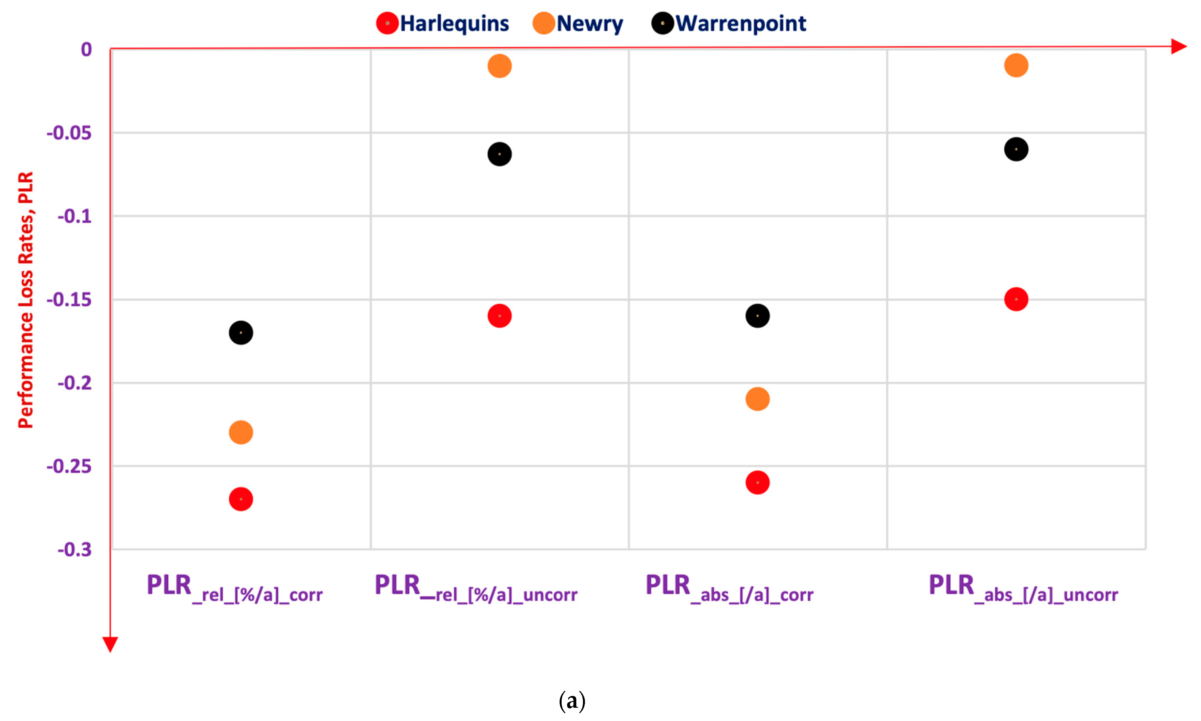
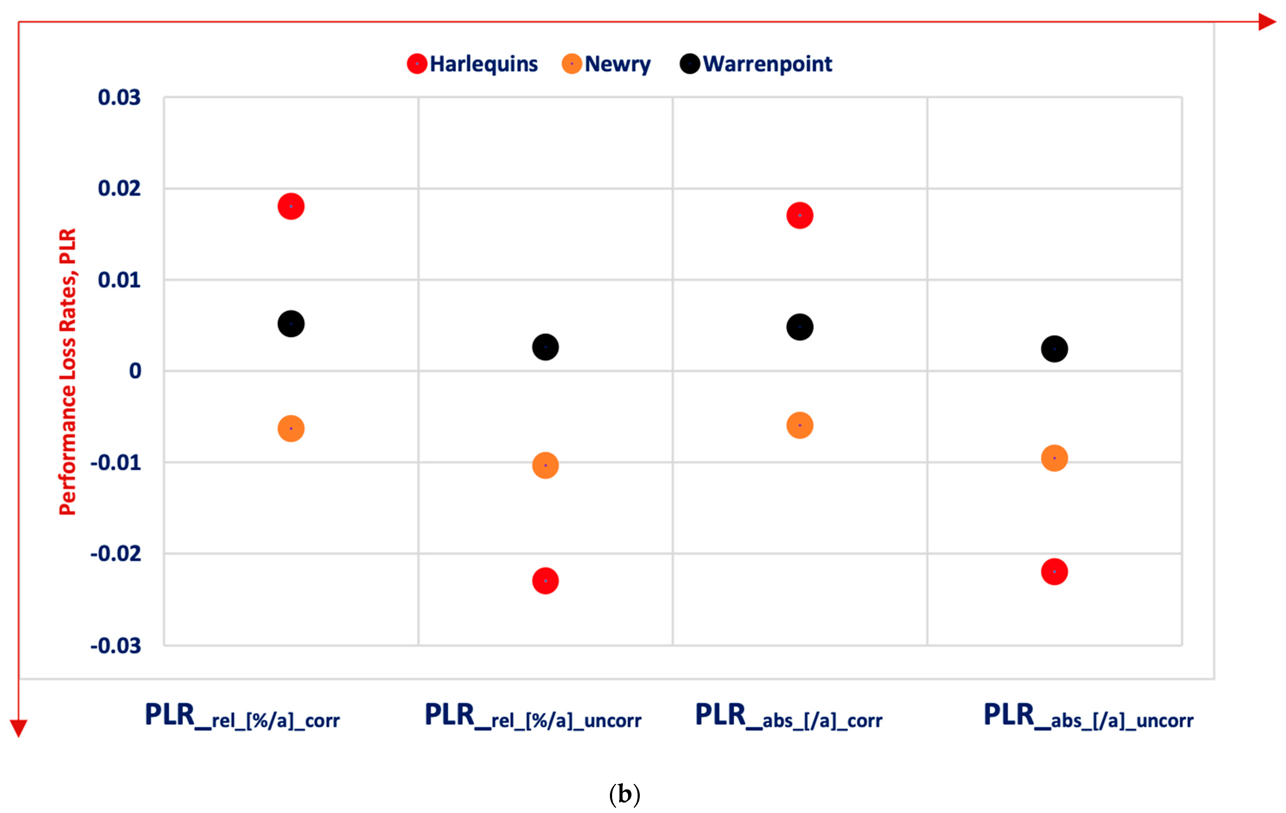
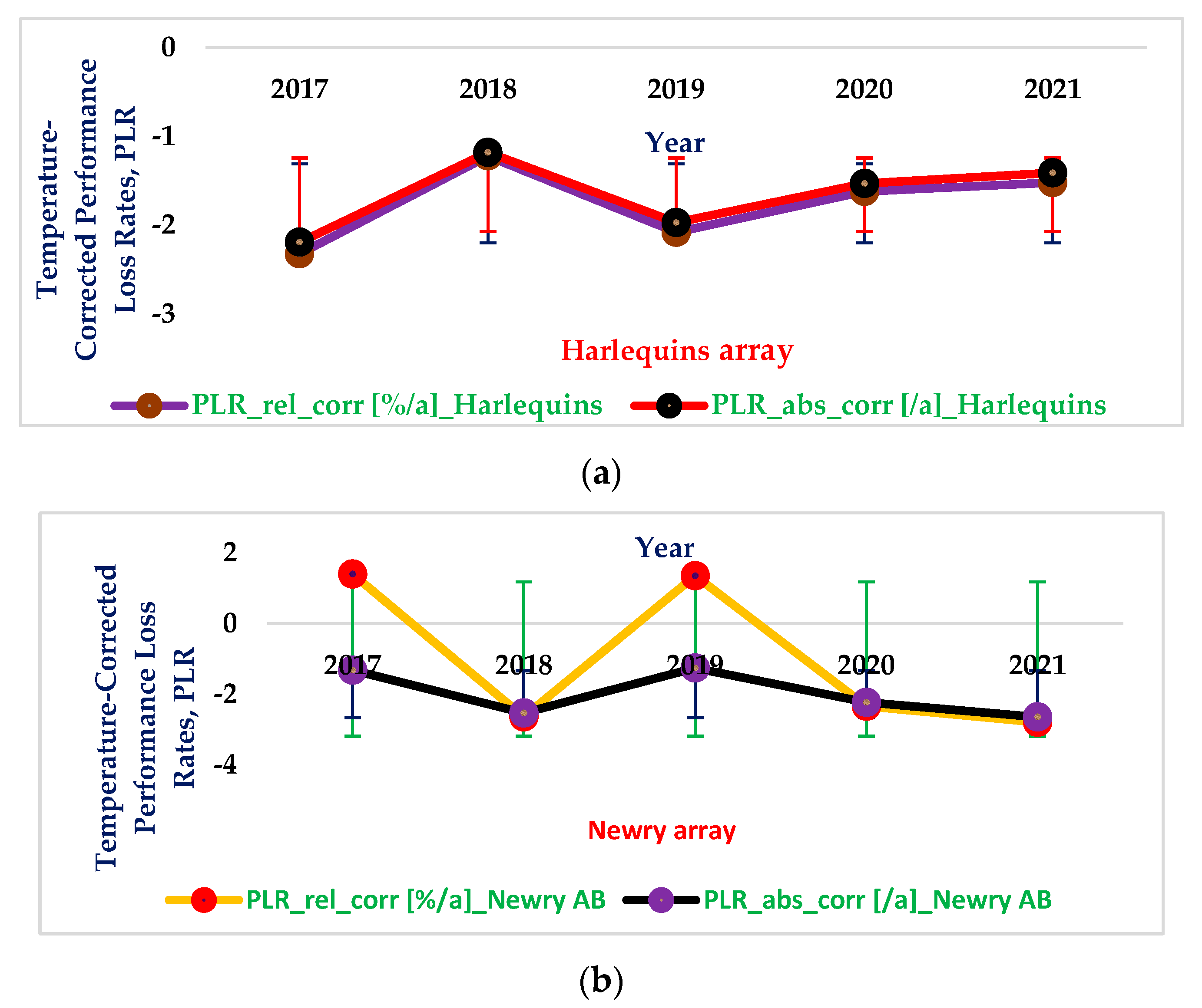
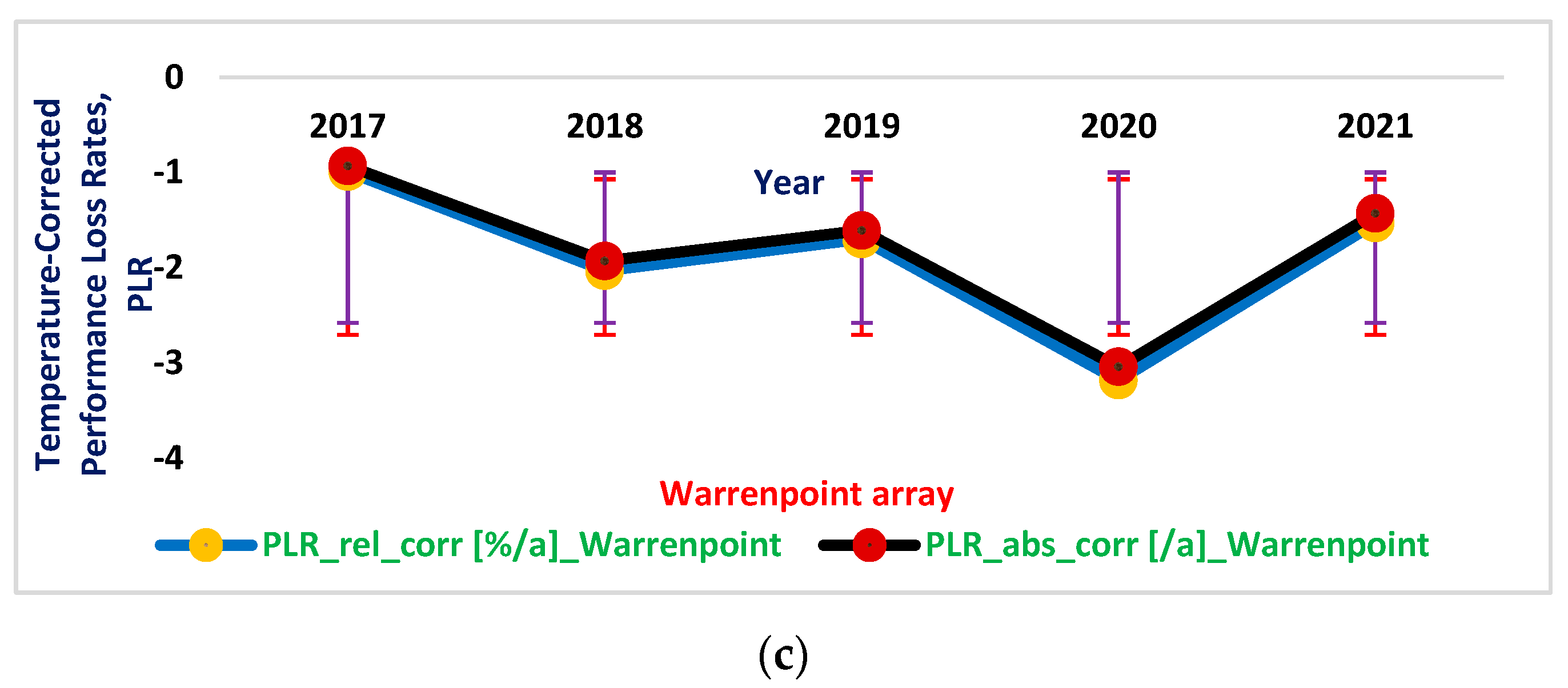
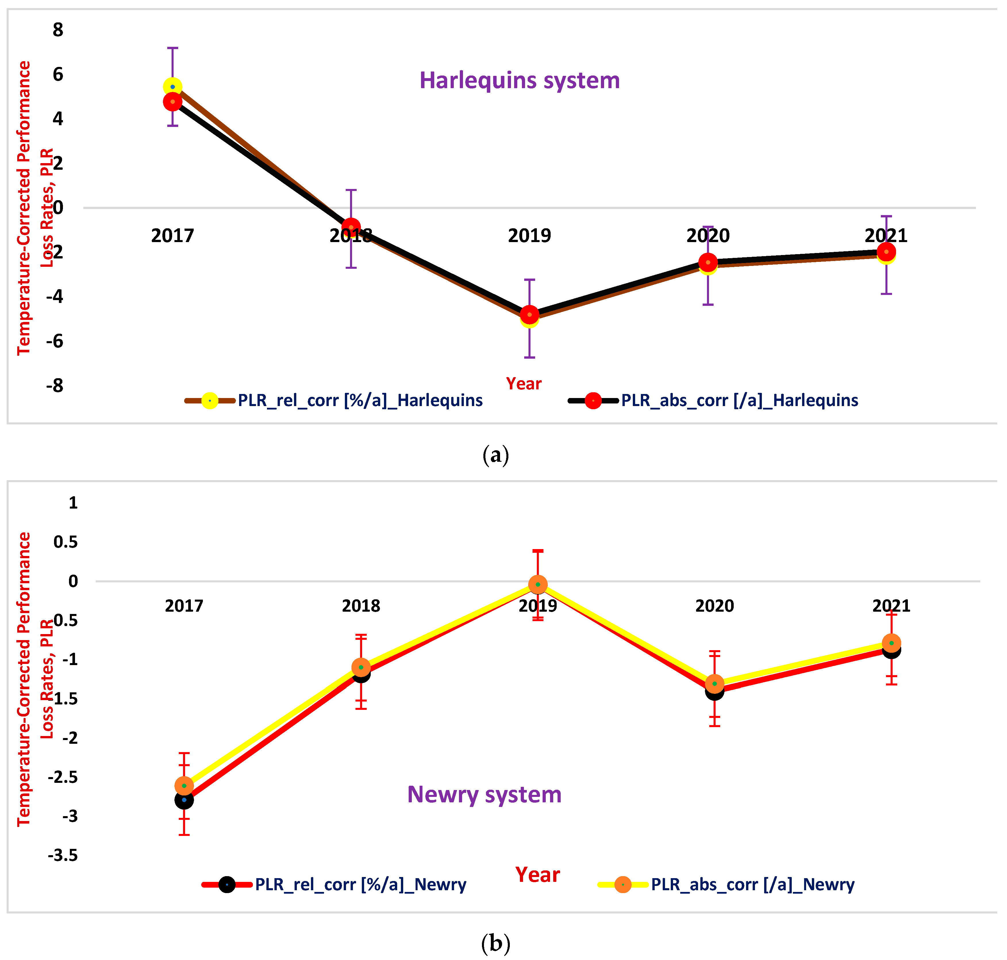
Arr. PLRrel (%/a)	Sys. PLRrel (%/a)	This means that PLRrel of the Harlequins array shows that solar panel generation will increase at the annual rate by −0.27%/a, which shows an improvement, while PLRrel of the Harlequins system shows that PV system generation will decrease at the annual rate of 0.018%/a.	Array PLRrel (%/a)	Sys. PLRrel (%/a)	There are improvements in both the Newry array and system. For this reason, both the PLRrel for the Newry array and system show that they will both increase at the annual rates by −0.23%/a and −0.00635%/a, respectively.	Arr. PLRrel (%/a)	Sys. PLRrel (%/a)	The PLRrel in Warrenpoint array shows that there is an improvement in the array. This means that solar panel generation will increase at an annual rate of −0.17%/a, while the PLRrel in the Warrenpoint system shows that PV system generation will decrease at the annual rate of 0.00514%/a.
−0.27	0.018		−0.23	−0.00635		−0.17	0.00514

,

Table A2. Temperature-correction for absolute performance loss rates (PLR_abs) for Harlequins, Newry, and Warrenpoint arrays and systems.

Harlequins		Observation	Newry		Observation	Warrenpoint		Observation
Arr. PLRabs (/a)	Sys. PLRabs (/a)	The PLRabs of the Harlequins array show that solar panel generation will increase at the annual rate of −0.26/a, which shows an improvement, while the PLRabs of the Harlequins system shows that PV system generation will decrease at the annual rate of 0.017/a.	Arr. PLRabs (/a)	Sys. PLRabs (/a)	Both the Newry array and system show improvements. This means that their PLRabs will increase at the annual rates by −0.21/a and −0.006/a, respectively.	Arr. PLRabs (/a)	Sys. PLRabs (/a)	Warrenpoint array shows a PLRabs improvement while the Warrenpoint system shows a decrease in PLR abs. This shows that solar panel generation will increase at an annual rate of −0.16/a, while the Warrenpoint system shows that PV system generation will decrease at an annual rate of 0.0048/a.
−0.26	0.017		−0.21	−0.006		−0.16	0.0048

,

Table A3. Weather-uncorrected relative performance loss rates (PLR_rel) for Harlequins, Newry, and Warrenpoint arrays and systems.

Harlequins		Observation	Newry		Observation	Warrenpoint		Observation
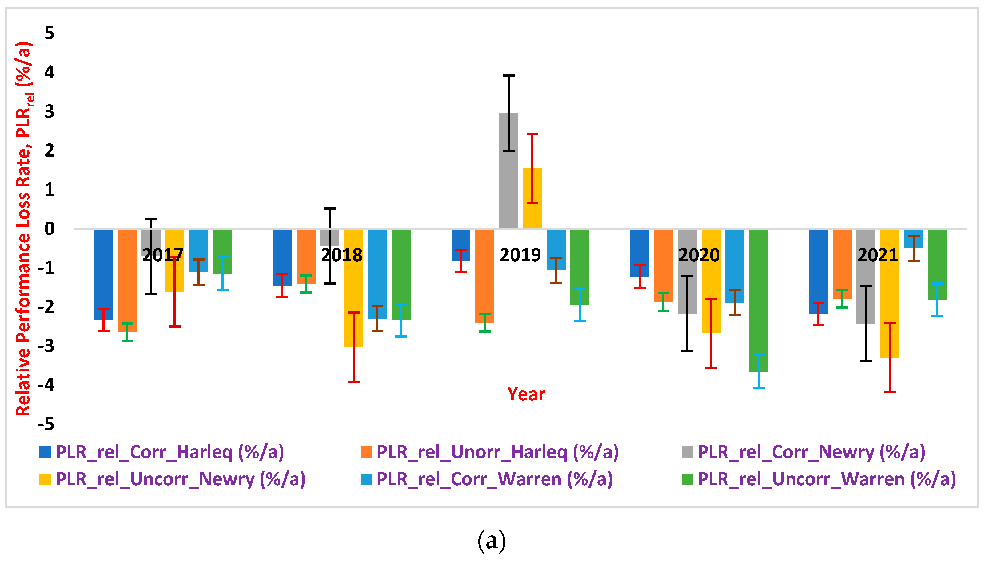
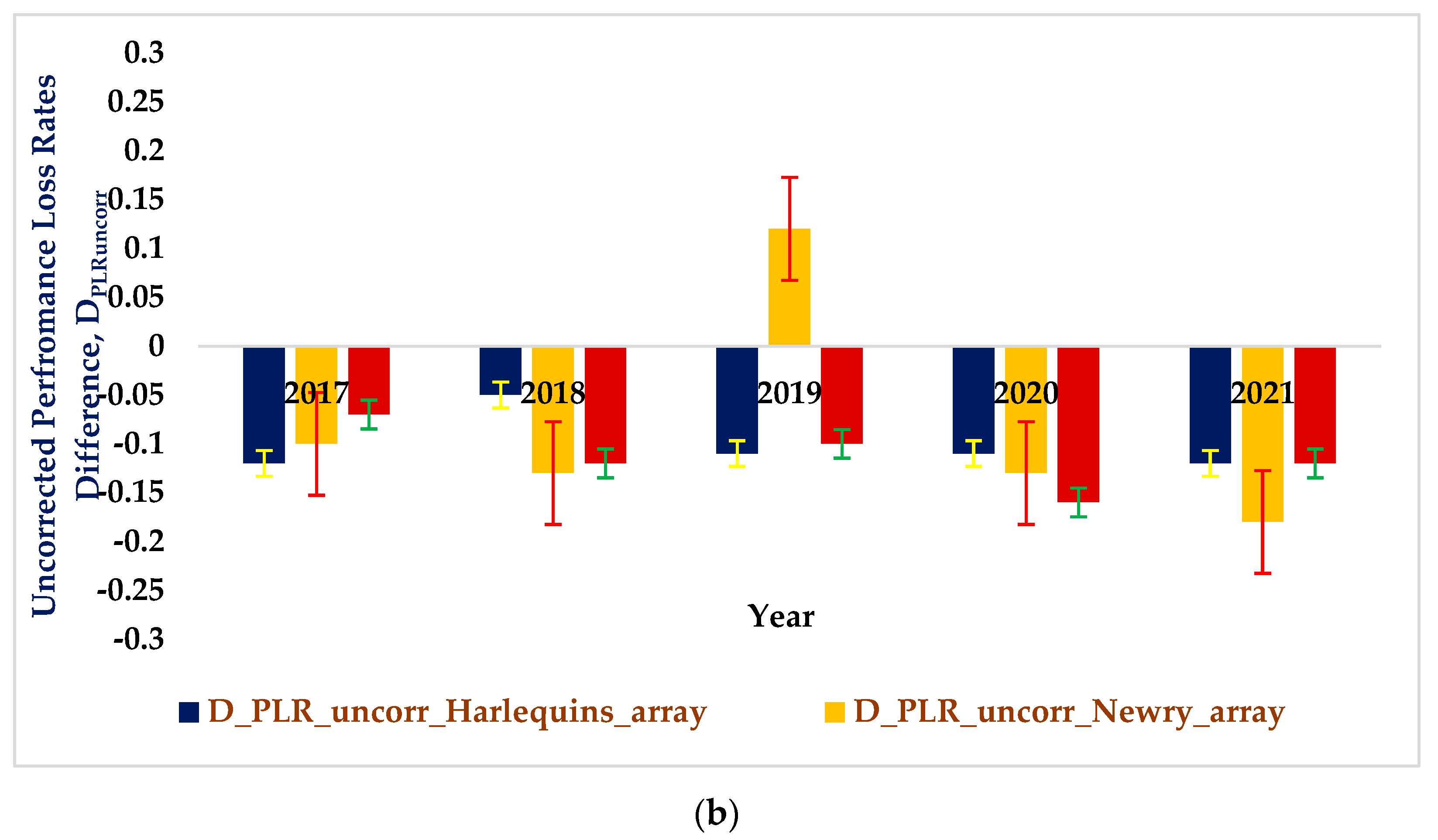
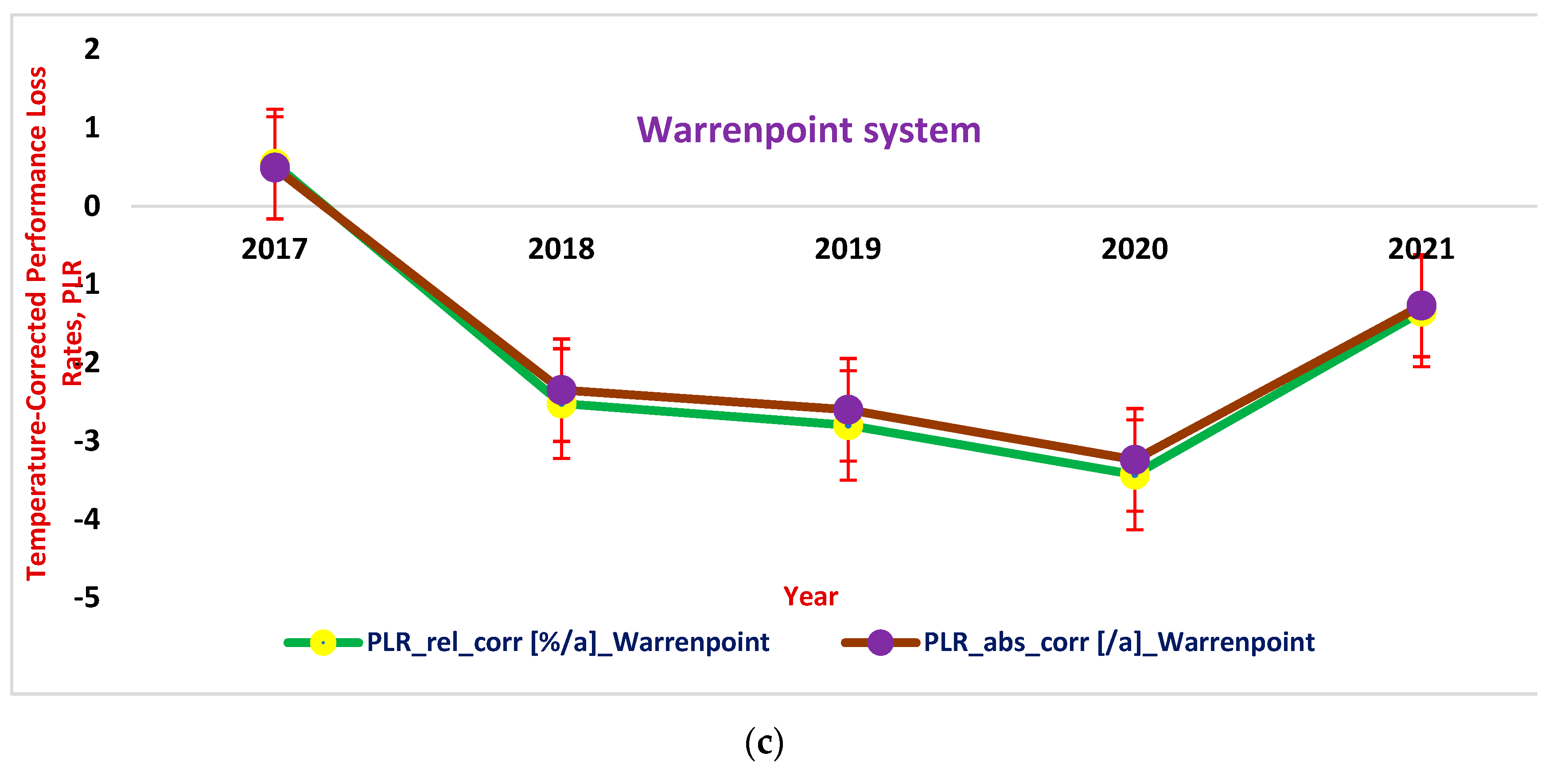
Arr. PLRrel (%/a)	Sys. PLRrel (%/a)	Both the Harlequins array and system showed an improvement at their PLRrel. This shows that solar panel and PV generations will increase at annual rates of −0.16%/a and −0.023%/a, respectively. It will be difficult to predict any PLRrel in the PV array and system due to the seasonal variation effect noticed in weather-uncorrected relative performance loss rates. To resolve this, the weather-uncorrected PLRrel are normalised with the average cell temperature.	Array PLRrel (%/a)	Sys. PLRrel (%/a)	There are improvements in the Newry array and system. For this reason, their PLRrel shows that both the Newry array and system will increase at the annual rates by −0.01%/a and −0.00104%/a, respectively. Just like the Harlequins array and system, it will be difficult to predict any PLRrel in the PV array and system due to the seasonal variation effect noticed in weather-uncorrected relative performance loss rates. To resolve this, the weather-uncorrected PLRrel are normalised with the average cell temperature.	Arr. PLRrel (%/a)	Sys. PLRrel (%/a)	There is an improvement in the Warrenpoint array and a decrease in the Warrenpoint system. This shows that solar panel generation will increase at an annual rate by −0.063%/a, while the Warrenpoint system shows that PV system generation will decrease at the annual rate of 0.00259%/a.
−0.16	−0.023		−0.01	−0.00104		−0.063	0.00259

and

Table A4. Weather-uncorrected absolute performance loss rates (PLR_abs) for Harlequins, Newry, and Warrenpoint arrays and systems.

Harlequins		Observation	Newry		Observation	Warrenpoint		Observation
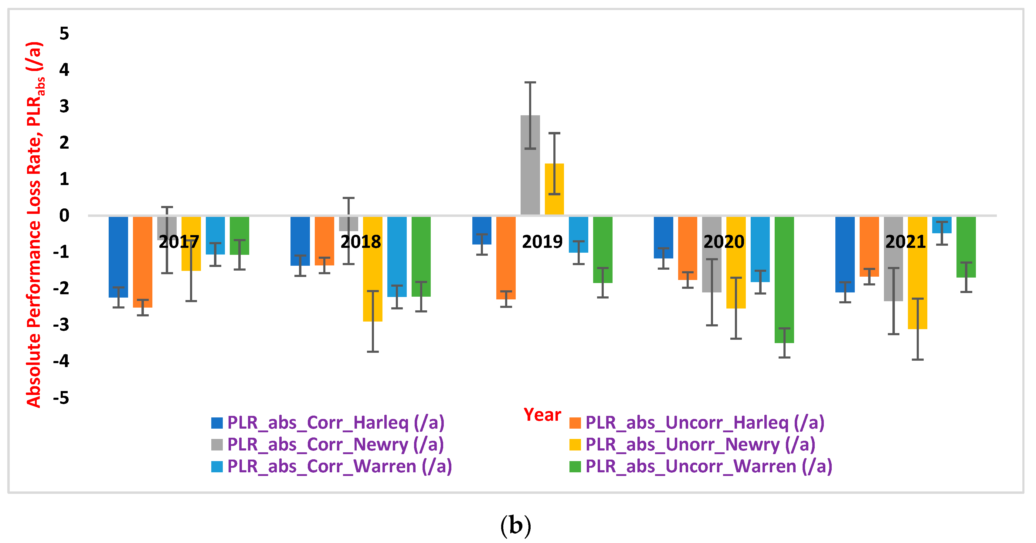
Arr. PLRabs (/a)	Sys. PLRabs (/a)	Both the Harlequins array and system show improvements in PLRabs. This show that solar panel and PV generations will increase at annual rates of −0.15/a and −0.022/a. Just like PLRrel in the Harlequins array and system, it will be difficult to predict any PLRrel in the PV array and system due to the seasonal variation effect noticed in weather-uncorrected relative performance loss rates. To resolve this, the weather-uncorrected PLRrel are normalised with the average cell temperature.	Arr. PLRabs (/a)	Sys. PLRabs (/a)	There are improvements in both the Newry array and system. This means that their PLRabs show that both the Newry array and system will increase at the annual rates by −0.0096/a and −0.0096/a, respectively. Just like the Newry array and system, it will be difficult to predict any PLRrel in the PV array and system due to the seasonal variation effect noticed in weather-uncorrected relative performance loss rates. To resolve this, the weather-uncorrected PLRrel are normalised with the average cell temperature.	Arr. PLRabs (/a)	Sys. PLRabs (/a)	Performance improvement is noticed in the Warrenpoint array and there is a decrease in performance in the Warrenpoint system. This means that solar panel generation will increase at an annual rate of −0.06/a, while the Warrenpoint system shows that PV system generation will decrease at the annual rate of 0.0024/a.
−0.15	−0.022		−0.0096	−0.0096		−0.06	0.0024

. The losses in a system are caused by various factors, including solar cell temperature losses, DC/AC inverter conversion losses, and solar radiation reflection losses. These losses can be further broken down into specific types of losses, such as shading losses, spectral losses, and inverter losses [44]. The following are some of the factors that contribute to system losses [44]: (i) Solar cell temperature losses: for every 1 °C above 25 °C, the output from a solar cell drops by 0.5%. (ii) DC/AC inverter conversion losses: PV inverter efficiency decreases from 0.3 to 1% per 150 V DC input voltage amplitude and the efficiency decreases down to 5% due to the power consumption of the control unit and switching losses. (iii) Solar radiation reflection losses: there is some loss of output around 2.5% when sunlight reflects off panel surfaces rather than being absorbed to generate electric current.

Figure 6a,b show the difference between the module temperature-corrected and uncorrected relative and absolute performance losses which are computed using (13) and (14):

D_PLRcorr = PLR_rel.corr − PLR_abs.module

(13)

D_PLRuncorr = PLR_rel.uncorr − PLR_abs.uncorr,

(14)

where D_{PLRcorr {}XE “D_PLRcorr:Differences in temperature-corrected performance loss rates in arrays and systems”_} and D_PLRuncorr{XE “D_PLRuncorr:Differences in uncorrected performance loss rates in arrays and systems.”_} are differences in temperature-corrected and uncorrected performance loss rates in arrays and systems. PLR_rel.corr{XE “PLR_rel.corr:Relative temperature-corrected performance loss rates in arrays and systems.”_} and PLR_rel.uncorr{XE “PLR_rel.uncorr:Relative uncorrected performance loss rates in arrays and systems.”_} are relative temperature-corrected and uncorrected performance loss rates in arrays and systems.

PLR_abs.corr{XE “PLR_abs.corr:Absolute temperature-corrected performance loss rates in arrays and systems”_} and PLR_abs.uncorr{XE “PLR_abs.uncorr:Absolute uncorrected performance loss rates in arrays and systems”_} are absolute temperature-corrected and uncorrected performance loss rates in arrays and systems.

To normalise relative and absolute temperature-corrected performance loss rate, the PLR_corr{XE “PLR_corr:Relative weather-corrected performance loss rate”_} from weather-uncorrected performance loss rate (PLR_uncorr{XE “PLR_Uncorr:Relative weather-corrected performance loss rate”_}) and the average cell temperatures, as shown in Table 2, for each PV array installed at Harlequins, Newry and Warrenpoint are used. Hence, the PLR_corr for PLR_rel and PLR_abs are normalised using Equations (15) and (16).

$${\mathrm{P}\mathrm{L}\mathrm{R}}_{\mathrm{c}\mathrm{o}\mathrm{r}\mathrm{r}\_\mathrm{r}\mathrm{e}\mathrm{l}}=\frac{{\mathrm{P}\mathrm{L}\mathrm{R}}_{\mathrm{u}\mathrm{n}\mathrm{c}\mathrm{o}\mathrm{r}\mathrm{r}\_\mathrm{r}\mathrm{e}\mathrm{l}}}{1-\frac{\mathsf{\delta }}{100}\left({\mathrm{T}\mathrm{c}\mathrm{e}\mathrm{l}\mathrm{l}}_{\mathrm{a}\mathrm{v}\mathrm{g}}\right)}$$

(15)

$${\mathrm{P}\mathrm{L}\mathrm{R}}_{\mathrm{c}\mathrm{o}\mathrm{r}\mathrm{r}\{}\mathrm{X}\mathrm{E}\mathrm{“}{\mathrm{P}\mathrm{L}\mathrm{R}}_{\mathrm{c}\mathrm{o}\mathrm{r}\mathrm{r}\_\mathrm{a}\mathrm{b}\mathrm{s}}:\mathrm{A}\mathrm{b}\mathrm{s}\mathrm{o}\mathrm{l}\mathrm{u}\mathrm{t}\mathrm{e} \mathrm{w}\mathrm{e}\mathrm{a}\mathrm{t}\mathrm{h}\mathrm{e}\mathrm{r}-\mathrm{c}\mathrm{o}\mathrm{r}\mathrm{r}\mathrm{e}\mathrm{c}\mathrm{t}\mathrm{e}\mathrm{d} \mathrm{p}\mathrm{e}\mathrm{r}\mathrm{f}\mathrm{o}\mathrm{r}\mathrm{m}\mathrm{a}\mathrm{n}\mathrm{c}\mathrm{e} \mathrm{l}\mathrm{o}\mathrm{s}\mathrm{s} \mathrm{r}\mathrm{a}\mathrm{t}\mathrm{e}\mathrm{s}{\mathrm{”}}_{\}}\_\mathrm{a}\mathrm{b}\mathrm{s}=\frac{{\mathrm{P}\mathrm{L}\mathrm{R}}_{\mathrm{u}\mathrm{n}\mathrm{c}\mathrm{o}\mathrm{r}\mathrm{r}\_\mathrm{a}\mathrm{b}\mathrm{s}}}{1-\frac{\mathsf{\delta }}{100}({\mathrm{T}\mathrm{c}\mathrm{e}\mathrm{l}\mathrm{l}}_{\mathrm{a}\mathrm{v}\mathrm{g}})}$$

(16)

4.5. Statistical Analyses Using t-Distribution and Confidence Intervals

Figure 7a–c and Figure 8a–c show graphs of module temperature-corrected relative performance loss rates, PLR_corr__rel, and module temperature-corrected absolute performance loss rates, PLR_corr__abs, across the three arrays and systems. The standard deviation error bars in these figures are overlapped because of the closeness of their standard deviation values, as shown in

Table 3. Comparative analysis of relative and absolute average and standard deviation of module temperature-corrected performance loss rates in arrays.

Harlequins				Newry				Warrenpoint
${\mathsf{\mu }}_{\mathrm{r}\mathrm{e}\mathrm{l}}$	${\mathsf{\sigma }}_{\mathrm{r}\mathrm{e}\mathrm{l}}$	${\mathsf{\mu }}_{\mathrm{a}\mathrm{b}\mathrm{s}}$	${\mathsf{\sigma }}_{\mathrm{a}\mathrm{b}\mathrm{s}}$	${\mathsf{\mu }}_{\mathrm{r}\mathrm{e}\mathrm{l}}$	${\mathsf{\sigma }}_{\mathrm{r}\mathrm{e}\mathrm{l}}$	${\mathsf{\mu }}_{\mathrm{a}\mathrm{b}\mathrm{s}}$	${\mathsf{\sigma }}_{\mathrm{a}\mathrm{b}\mathrm{s}}$	${\mathsf{\mu }}_{\mathrm{r}\mathrm{e}\mathrm{l}}$	${\mathsf{\sigma }}_{\mathrm{r}\mathrm{e}\mathrm{l}}$	${\mathsf{\mu }}_{\mathrm{a}\mathrm{b}\mathrm{s}}$	${\mathsf{\sigma }}_{\mathrm{a}\mathrm{b}\mathrm{s}}$
−1.75	0.44	−1.66	0.41	−1.00	2.17	−1.99	0.66	−1.89	0.81	−1.79	0.79

and

Table 4. Relative and absolute average and standard deviation values of module temperature corrected performance loss rates in systems.

Harlequins				Newry				Warrenpoint
${\mathsf{\mu }}_{\mathrm{r}\mathrm{e}\mathrm{l}}$	${\mathsf{\sigma }}_{\mathrm{r}\mathrm{e}\mathrm{l}}$	${\mathsf{\mu }}_{\mathrm{a}\mathrm{b}\mathrm{s}}$	${\mathsf{\sigma }}_{\mathrm{a}\mathrm{b}\mathrm{s}}$	${\mathsf{\mu }}_{\mathrm{r}\mathrm{e}\mathrm{l}}$	${\mathsf{\sigma }}_{\mathrm{r}\mathrm{e}\mathrm{l}}$	${\mathsf{\mu }}_{\mathrm{a}\mathrm{b}\mathrm{s}}$	${\mathsf{\sigma }}_{\mathrm{a}\mathrm{b}\mathrm{s}}$	${\mathsf{\mu }}_{\mathrm{r}\mathrm{e}\mathrm{l}}$	${\mathsf{\sigma }}_{\mathrm{r}\mathrm{e}\mathrm{l}}$	${\mathsf{\mu }}_{\mathrm{a}\mathrm{b}\mathrm{s}}$	${\mathsf{\sigma }}_{\mathrm{a}\mathrm{b}\mathrm{s}}$
−1.04	3.91	−1.06	3.57	−1.26	1.00	−1.17	0.94	−1.91	1.56	−1.79	1.46

.

Above, µ_rel{XE “µ_rel:Relative averages of the temperature-corrected performance loss rates”_} and µ_abs{XE “µ_abs:Absolute averages of the temperature-corrected performance loss rates”_} are relative and absolute averages of the module temperature-corrected performance loss rates, while $\mathsf{\sigma }$_rel{XE “$\mathsf{\sigma }$_rel:Relative standard deviations of the temperature-corrected performance loss rates”_} and $\mathsf{\sigma }$_abs{XE “$\mathsf{\sigma }$_abs:Absolute standard deviations of the temperature-corrected performance loss rates”_} are relative and absolute standard deviations of the module temperature-corrected performance loss rates.

The test of significance for relative and absolute temperature-corrected performance loss rates across the three sites is computed using Equation (17).

$${\mathrm{t}}_{\mathrm{c}\mathrm{a}\mathrm{l}}=\frac{\sum \mathrm{di}}{\sqrt{\frac{{\mathrm{n}(\sum \mathrm{di}}^2)-(\sum {\mathrm{di})}^2}{\mathrm{DF}}}},$$

(17)

where di{XE “di:Difference between corrected absolute and relative performance loss rates”} = PLR_{corr_abs} − PLR_{corr_rel}.

(18)

n = 5 is the number of monitored data points.

DF{XE “DF:Degree of freedom”} = n − 1 is the degree of freedom.

t_cal{XE “t_cal:Calculated t-value”_} is the calculated t-value.

PLR_abs__corr is the absolute weather-corrected performance loss rate.

PLR_rel__corr is the relative weather-corrected performance loss rate.

Calculated t-values (t_cal) for Harlequins and Warrenpoint arrays for temperature-corrected performance loss rates are greater than the critical values, t_critical (t_cal > t_critical), at 0.05, 0.10, and 0.01 levels of significance, and the Newry array t_cal value is less than the critical value, t_critical (t_cal < t_critical), at 0.05, 0.10, and 0.01 levels of significance, while t_cal for the Harlequins system for temperature-corrected performance loss rates is less than the critical values, t_critical (t_cal < t_critical), at 0.05, 0.10, and 0.01 levels of significance. This is shown in the t-distribution statistical table in

Table 5. Test of significance for the temperature-corrected performance loss rates in Harlequins, Newry, and Warrenpoint arrays and systems.

tcritical at Level of Significance, α	tcal for Harlequins		tcal for Newry		tcal for Warrenpoint
	Array	System	Array	System	Array	System
${\mathsf{\alpha }}_{0.05}=2.13$	6.24	−0.15	−1.45	3.10	7.65	2.51
${\mathsf{\alpha }}_{0.10}=1.53$	6.24	−0.15	−1.45	3.10	7.65	2.51
${\mathsf{\alpha }}_{0.01}=3.74$	6.24	−0.15	−1.45	3.10	7.65	2.51

. Warrenpoint and Newry systems are significant at 0.05 and 0.10 because t_cal > t_critical, while they are not significant at 0.01 because t_cal < t_critical. This means that the difference, d_i, between the PLR_{abs_corr} and PLR_{rel_corr} for the Harlequins array, Warrenpoint array, and Newry system are all significant at 0.05, 0.10, and 0.01 because t_cal > t_critical, while the Harlequins system and Newry array are not significant because t_cal < t_critical. The Warrenpoint system is only significant at 0.05 and 0.10 using Equation (17).

A paired t-test, utilising the t-distribution, was employed to assess the significance of temperature correction in mitigating seasonal fluctuations of the performance ratios. The assessment was conducted at various significance levels ($\alpha$ = 0.05, 0.10, and 0.01) and confidence intervals (C.I = 95%, 90% and 99%). The statistical analysis outcome indicates that for the Harlequins, Newry, and Warrenpoint PV arrays, the calculated t-values (t_cal) for $\alpha$ = 0.05, 0.10, and 0.01, as shown in

Table 6. Statistical analysis for Harlequins, Newry, and Warrenpoint systems.

			Harlequins			Newry				Warrenpoint
α	tcritical	dmean	$\mathsf{\Sigma }$	S.E(dmean)	tcal	dmean	$\mathsf{\sigma }$	S.E(dmean)	tcal	dmean	$\mathsf{\sigma }$	S.E(dmean)	tcal
0.05	2.00	1.91	4.85	0.63	3.04	1.70	4.74	0.61	2.80	1.85	4.67	0.60	3.06
0.10	1.67
0.01	2.66

, demonstrate statistical significance, leading to the rejection of the null hypothesis (H₀) and the acceptance of the alternative hypothesis (H₁). Figure 9 illustrates the confidence intervals (C.I) at 95%, 90%, and 99%, aligning with the confidence levels reported for t_cal values in Table 6 across the three PV arrays. Notably, the standard error of the mean difference (SE(d_mean)) displayed in Figure 9, along with t_cal, remains consistent. This consistency is anticipated since physically similar PV arrays should exhibit akin S.E (d_mean) and t_cal values. The congruence between S.E (d_mean) and t_cal values provides compelling evidence that the implementation of module temperature correction effectively diminishes seasonal performance ratio variations. As a result, an enhancement in PV performance is achieved.

Above, α is the level of significance; d_mean is the mean difference; $\mathsf{\sigma }$ is the standard deviation; t_cal is the calculated t-value; S.E(d_mean) is the standard error of the mean difference; DF = n − 1 is the degree of freedom; n = 60 is the number of monitored data points; and T_C.I is the t-test at a particular confidence interval (C.I).

5. Discussion

The discussion on “disaggregating longer-term trends from seasonal variations in measured PV system performance” revolves around the exploration of a method or approach that aims to separate and analyse the longer-term trends in the performance of PV systems from the shorter-term variations. This type of analysis is crucial for understanding the overall performance of PV systems, identifying underlying factors that affect performance changes over time and making informed decisions for system optimisation. This study introduced a novel methodology that allows for the decomposition of measured PV system performance data into two main components: longer-term trends and seasonal variations. This separation enables a more detailed and accurate examination of the factors that influence PV system performance. In this discussion, several key points are typically addressed: (i) Overview of the Methodology: This study provides a concise summary of the method developed to disaggregate the longer-term trends and seasonal variations in PV system performance. This includes appropriate mathematical equations and statistical techniques used to achieve this separation. (ii) Significance of Longer-Term Trends: The study discusses the importance of understanding the longer-term trends in PV system performance. These trends are indicative of factors such as degradation, efficiency improvements, technological advancements, and changing environmental conditions over the years. (iii) Seasonal Variations: The study delved into the significance of seasonal variations in PV system performance. These variations are influenced by factors such as solar irradiance, temperature, shading, and maintenance practices. Hence, understanding these variations is crucial for optimising system performance.

6. Conclusions

The PV performance ratios underwent adjustments utilising the average annual cell temperature (T_{Cell_avg}), leading to the acquisition of performance ratios that have been rectified for module temperature. Through the utilisation of data gathered from a five-year examination involving three arrays, a comprehensive statistical investigation was conducted employing paired t-tests and confidence intervals. The primary goal was to ascertain the extent to which the variation in seasonal performance ratios decreased due to the module temperature correction. This investigation encompassed 95%, 90%, and 99% confidence intervals (C.I), alongside significance levels of 0.05, 0.10, and 0.01. Remarkably, the confidence values of C.I, t_cal values, and S.E(d_mean) demonstrated consistency, reflecting the similarity of the PV arrays. As a consequence of this observed similarity, the outcome of PR_corr exhibited more pronounced enhancement when compared to PR_uncorr.

References

- Okorieimoh, C. Long-Term Durability of Rooftop Grid-Connected Solar Photovoltaic Systems. Ph.D. Thesis, Technological University Dublin, Dublin, Ireland, 2022. Available online: https://arrow.tudublin.ie/engdoc/140/ (accessed on 8 April 2022).
- Lindig, S.; Theristis, M.; Moser, D. Best Practices for Photovoltaic Performance Loss Rate Calculations. Prog. Energy 2022, 4, 022003. [Google Scholar] [CrossRef]
- Dierauf, T.; Growitz, A.; Kurtz, S.; Becerra Cruz, J.L.; Riley, E.; Hansen, C. Weather-Corrected Performance Ratio; National Renewable Energy Laboratory NREL: Golden, CO, USA, 2013.
- Shravanth Vasisht, M.; Srinivasan, J.; Ramasesha, S.K. Performance of solar photovoltaic installations: Effect of seasonal variations. Sol. Energy 2016, 131, 39–46. [Google Scholar] [CrossRef]
- Sunnova. How Energy Use and Seasonal Changes Affect Your Solar Panel Output. 2022. Available online: https://www.sunnova.com/watts-up/home-solar-seasonality (accessed on 8 April 2022).
- Solar, I. Seasonal Variations in Solar Panel Performance. 2023. Available online: https://insolationenergy.in/seasonal-variations-in-solar-panel-performance/ (accessed on 14 February 2023).
- Okorieimoh, C.C.; Norton, B.; Conlon, M. The Effects of the Transient and Performance Loss Rates on PV Output Performance. In Proceedings of the International Conference on Innovations in Energy Engineering & Cleaner Production IEECP21, Silicon Valley, San Francisco, CA, USA, 29–30 July 2021. [Google Scholar]
- Aboagye, B.; Gyamfi, S.; Ofosu, E.A.; Djordjevic, S. Degradation analysis of installed solar photovoltaic (PV) modules under outdoor conditions in Ghana. Energy Rep. 2021, 7, 6921–6931. [Google Scholar] [CrossRef]
- Chandel, S.; Naik, M.N.; Sharma, V.; Chandel, R. Degradation analysis of 28-year field exposed mono-c-Si photovoltaic modules of a direct coupled solar water pumping system in western Himalayan region of India. Renew. Energy 2015, 78, 193–202. [Google Scholar] [CrossRef]
- Jordan, D.C.; Deline, C.; Kurtz, S.R.; Kimball, G.M.; Anderson, M. Robust PV Degradation Methodology and Application. IEEE J. Photovolt. 2018, 8, 525–531. [Google Scholar] [CrossRef]
- Köntges, M.; Kurtz, S.; Packard, C.E.; Jahn, U.; Berger, K.A.; Kato, K.; Friesen, T.; Liu, H.; Van Iseghem, M.; Wohlgemuth, J.; et al. Review of Failures of Photovoltaic Modules; IEA International Energy Agency: Paris, France, 2014. [Google Scholar]
- Duffie, J.A.; Beckman, W.A. Solar Engineering of Thermal Processes; John Wiley & Sons: Hoboken, NJ, USA, 2013. [Google Scholar]
- Skoplaki, E.; Palyvos, J. On the temperature dependence sof photovoltaic module electrical performance: A review of efficiency/power correlations. Sol. Energy 2009, 83, 614–624. [Google Scholar] [CrossRef]
- Lorenzo, E.; Zarza, E. Performance assessment of parabolic trough solar power plants. Sol. Energy 2003, 74, 217–232. [Google Scholar]
- King, D.L.; Boyson, W.E.; Kratochvil, J.A. Photovoltaic Array Performance Model. Sandia National Laboratories Report 2004 (SAND2004-3535). Available online: http://www.osti.gov/servlets/purl/919131-sca5ep/ (accessed on 1 August 2004).
- Kara, E.C.; Roberts, C.M.; Tabone, M.; Alvarez, L.; Callaway, D.S.; Stewart, E.M. Disaggregating solar generation from feeder-level measurements. Sustain. Energy Grids Netw. 2018, 13, 112–121. [Google Scholar] [CrossRef]
- Ayob, A. Solar PV Monitoring. Scholarly Community Encyclopedia. 2021. Available online: https://encyclopedia.pub/entry/13058 (accessed on 12 August 2021).
- Woyte, A.; Richter, M.; Moser, D.; Reich, N.; Green, M.; Mau, S.; Georg Beyer, H. Analytical Monitoring of Grid-Connected Photovoltaic Systems, Good Practices for Monitoring and Performance Analysis; International Energy Agency Photovoltaic Power Systems Programme (IEA PVPS): Bundestag, Germany, 2014. [Google Scholar]
- Mau, S.; Jahn, U. Performance Analysis of Grid-Connected PV Systems; IEA PVPS: Vienna, Austria, 2006. [Google Scholar]
- Tahri, F.; Tahri, A.; Oozeki, T. Performance evaluation of grid-connected photovoltaic systems based on two photovoltaic module technologies under tropical climate conditions. Energy Convers. Manag. 2018, 165, 244–252. [Google Scholar] [CrossRef]
- Hioki, A.T.; da Silva, V.R.G.R.; Junior, J.A.V.; Loures, E.d.F.R. Performance Analysis of Small Grid Connected Photovoltaic Systems. Braz. Arch. Biol. Technol. 2019, 62, 19190018. [Google Scholar] [CrossRef]
- Jahn, U.; Nasse, W. Operational performance of grid-connected PV systems on buildings in Germany. Prog. Photovolt. Res. Appl. 2004, 12, 441–448. [Google Scholar] [CrossRef]
- Stettler, S.; Toggweiler, P.; Wiemken, E.; Heydenreich, W.; de Keizer, A.C.; van Sark, W.; Feige, S.; Schneider, M.; Heilscher, G.; Lorenz, E. Failure detection routine for grid-connected PV systems as part of the PVSAT-2 project. In Proceedings of the 20th European Photovoltaic Solar Energy Conference, Barcelona, Spain, 6–10 June 2005. [Google Scholar]
- Drews, A.; De Keizer, A.C.; Beyer, H.G.; Lorenz, E.; Betcke, J.; Van Sark, W.; Heydenreich, W.; Wiemken, E.; Stettler, S.; Toggweiler, P. Monitoring and remote failure detection of grid-connected PV systems based on satellite observations. Sol. Energy 2007, 81, 548–564. [Google Scholar] [CrossRef]
- de Keizer, A.C.; van Sark, W.; Stettler, S.; Toggweiler, P.; Lorenz, E.; Drews, A.; Heinemann, D.; Heilscher, G.; Schneider, M.; Wiemken, E. PVSAT-2: Results of field test of the satellite-based PV system performance check. In Proceedings of the 21st European Photovoltaic Solar Energy Conference, Dresden, Germany, 4–8 September 2006. [Google Scholar]
- Carl Von Ossietzky Universitat Oldenburg. “PVSAT-2,” PVSAT-2: Weather Satellites Help Improving PV System Performance. 2009. Available online: https://studylib.net/doc/12028791/analytical-monitoring-of-grid-connected-photovoltaic-systems (accessed on 10 July 2009).
- Jiaying, Y.; Thomas, R.; Joachim, L. Seasonal variation of PV module performance in tropical regions. In Proceedings of the 38th IEEE Photovoltaic Specialists Conference, Austin, TX, USA, 3–8 June 2012. [Google Scholar]
- Carr, A.J.; Pryor, T.L. A comparison of the performance of different PV module types in temperate climates. Sol. Energy 2004, 76, 285–294. [Google Scholar] [CrossRef]
- Nakajima, A.; Ichikawa, M.; Kondo, M.; Yamamoto, K.; Yamagishi, H.; Tawada, Y. Spectral Effects of a Single-Junction Amorphous Silicon Solar Cell on Outdoor Performance. Jpn. J. Appl. Phys. 2004, 43, 2425. [Google Scholar] [CrossRef]
- Osterwald, C.; Anderberg, A.; Rummel, S.; Ottoson, L. Degradation analysis of weathered crystalline-silicon PV modules. In Proceedings of the Conference Record of the Twenty-Ninth IEEE Photovoltaic Specialists Conference, New Orleans, LA, USA, 19–24 May 2002. [Google Scholar]
- Tiwari, G.; Mishra, R.; Solanki, S. Photovoltaic modules and their applications: A review on thermal modelling. Appl. Energy 2011, 88, 2287–2304. [Google Scholar] [CrossRef]
- Magare, D.B.; Sastry, O.S.; Gupta, R.; Betts, T.R.; Gottschalg, R.; Kumar, A.; Bora, B.; Singh, Y.K. Effect of seasonal spectral variations on performance of three different photovoltaic technologies in India. Int. J. Energy Environ. Eng. 2016, 7, 93–103. [Google Scholar] [CrossRef]
- Quansah, D.A.; Adaramola, M.S. Assessment of early degradation and performance loss in five co-located solar photovoltaic module technologies installed in Ghana using performance ratio time-series regression. Renew. Energy 2019, 131, 900–910. [Google Scholar] [CrossRef]
- Theristis, M.; Livera, A.; Jones, C.B.; Makrides, G.; Georghiou, G.E.; Stein, J.S. Nonlinear Photovoltaic Degradation Rates: Modeling and Comparison Against Conventional Methods. IEEE J. Photovolt. 2020, 10, 1112–1118. [Google Scholar] [CrossRef]
- Chegaar, M.; Hamzaoui, A.; Namoda, A.; Petit, P.; Aillerie, M.; Herguth, A. Effect of Illumination Intensity on Solar Cells Parameters. Energy Procedia 2013, 36, 722–729. [Google Scholar] [CrossRef]
- Razak, A.; Irwan, Y.; Leow, W.; Irwanto, M.; Safwati, I.; Zhafarina, M. Investigation of the Effect Temperature on Photovoltaic (PV) Panel Output Performance. Int. J. Adv. Sci. Eng. Inf. Technol. 2016, 6, 682. [Google Scholar] [CrossRef]
- Stowell, D.; Kelly, J.; Tanner, D.; Taylor, J.; Jones, E.; Geddes, J.; Chalstrey, E. A harmonised, high-coverage, open dataset of solar photovoltaic installations in the UK. Sci. Data 2020, 7, 394. [Google Scholar] [CrossRef] [PubMed]
- Kani, S.A.P.; Wild, P.; Saha, T.K. Improving Predictability of Renewable Generation Through Optimal Battery Sizing. IEEE Trans. Sustain. Energy 2018, 11, 37–47. [Google Scholar] [CrossRef]
- Chiang, P.-H.; Chiluvuri, S.P.V.; Dey, S.; Nguyen, T.Q. Forecasting of Solar Photovoltaic System Power Generation Using Wavelet Decomposition and Bias-Compensated Random Forest. In Proceedings of the 9th IEEE Green Technology Conference, Denver, CO, USA, 29–31 March 2017; pp. 260–266. [Google Scholar]
- French, R.; Bruckman, L.; Moser, D.; Lindig, S.; Van Iseghem, M.; Müller, B.; Stein, J.; Richter, M.; Herz, M.; Sark, W.; et al. Assessment of Performance Loss Rate of PV Systems; International Energy Agency, Fraunhofer ISE: Freiburg, Germany, 2021. [Google Scholar]
- Okello, D.; Vorster, F.; van Dyk, E.E. Analysis of measured and simulated performance data of a 3.2 kWp grid-connected PV system in Port Elizabeth, South Africa. Energy Convers. Manag. 2015, 100, 10–15. [Google Scholar] [CrossRef]
- Ingenhoven, P.; Belluardo, G.; Moser, D. Comparison of Statistical and Deterministic Smoothing Methods to Reduce the Uncertainty of Performance Loss Rate Estimates. IEEE J. Photovolt. 2017, 8, 224–232. [Google Scholar] [CrossRef]
- Dhimish, M.; Alrashidi, A. Photovoltaic Degradation Rate Affected by Different Weather Conditions: A Case Study Based on PV Systems in the UK and Australia. Electronics 2020, 9, 650. [Google Scholar] [CrossRef]
- Veiga, A. Ultimate Guide to Utility-Scale PV System Losses; Rated Power: Madrid, Spain, 2022. [Google Scholar]