Article

Energy-Loss Straggling and Delta-Ray Escape in Solid-State Microdosimeters Used in Ion-Beam Therapy

1
MedAustron Ion Therapy Center, 2700 Wiener Neustadt, Austria
2
Department of Radiation Oncology, Medical University of Vienna, 1090 Vienna, Austria
3
Radiation Physics, Technische Universität Wien, 1040 Vienna, Austria
4
Centre for Medical Radiation Physics, University of Wollongong, Wollongong, NSW 2522, Australia
5
National Physical Laboratory, Teddington TW11 0LW, UK
*
Author to whom correspondence should be addressed.
J. Nucl. Eng. 2022, 3(2), 128-151; https://doi.org/10.3390/jne3020008
Submission received: 7 March 2022 / Revised: 26 April 2022 / Accepted: 30 April 2022 / Published: 6 May 2022
(This article belongs to the Special Issue Recent Advances in Applied Nuclear and Radiation Physics)

Abstract

:
Microdosimetry is increasingly adopted in the characterization of proton and carbon ion beams used in cancer therapy. Spectra and mean values of lineal energy calculated in frequency and dose are seen by many as the tools which, by complementing dosimetric measurements, allow for the most complete characterization of the therapeutic radiation fields. The urgency is now to consolidate the experience and converge to commonly accepted methodologies. In this context, the purpose of this work is to study the effects of the energy-loss straggling and the delta-ray escape, considering slab-sensitive volumes; these are, in fact, the typical shapes of solid-state microdosimeters, which are widely used in investigating light ion therapy beams. The method considers the energy distribution of delta rays resulting from the collision of the impinging ion and, taking into account the escape, convolutes it with itself as many times as the expected number of collisions in the sensitive volume thickness. The resulting distribution is compared to the experimental microdosimetric spectrum showing a substantially good agreement. The extension of the methodology to a wider range of ion energy and detector characteristics is instrumental for a detector-independent microdosimetric assessment of the radiation fields.

1. Introduction

In the wake of the rising interest to use proton and carbon ion beams for cancer therapy, numerous microdosimetric investigations for the characterization of these beam types have been reported. The reason for these experimental studies is the correlation of lineal energy spectra with the characteristic increase in biological effectiveness that light ions show at the end of their path. After several major studies conducted around the world, investigations are now more mature, collections of lineal energy spectra directly in clinical beams are more systematic, and the goal has become more ambitious: to provide detector-independent characterizations of the radiation. This is not an easy task as the microdosimeters used are different in size, material, shape, and radiation detection processes. Furthermore, there is no common methodological standard. In this transition phase, it is important to reconsider the basics and try to give interpretations of the microdosimetric outcomes by referring to the fundamental quantities and processes of physics.
In this framework, this work studies the influence of energy-loss straggling and delta-ray escape on microdosimetric spectra collected with slab solid-state detectors under the radiation of carbon ions. The impact that energy-loss straggling and delta-ray escape have on microdosimetric spectra was already the subject of Rossi’s pioneering studies [1], and a quantitative analysis was proposed more than fifty years ago by Kellerer [2]. However, no specific references were provided in these investigations to therapeutic ion beams of energies of hundreds of MeV per nucleon and solid-state microdosimeters, since such treatment modalities and detectors were, at the time, in their infancy.
In this work, the energy-loss straggling is investigated using recursive auto-convolutions of the distribution of the energy transferred in the individual collision of an ion and an electron. This method, originally adopted for spherical gas detectors by Kellerer, is revisited by considering slab microdosimeters. The procedure is applied to two specific cases of carbon ion irradiation, with beams of 279.8 MeV·u−1 and 207.8 MeV·u−1 and a silicon microdosimeter with slab sensitive volume (SV), with a circular cross-section of 30 µm in diameter and 10 µm in thickness. The computational results are compared with experimental data collected at those carbon ion energies in the MedAustron ion therapy center using the so-called “3D mushroom” silicon microdosimeter of the University of Wollongong with the geometric characteristics mentioned. The electronic collision distribution provided by Rutherford [3] is modified and simplified to take into account the limit to the maximum energy of the delta ray, the binding energy of the electrons, and the effects of delta-ray escape. Two distributions result from this process: the first is used to estimate the distribution of the energy loss and the second to estimate the distribution of the energy imparted in microdosimeters.

2. Materials and Methods

2.1. Method: Manipulation of the Collision Distributions

The energy loss straggling is the result of two contributions, one represented by the probability that the primary particle collides with the electrons of the medium and the other by the distribution of the energy lost in the single collision. Neglecting nuclear reactions and Bremsstrahlung and assuming that the binding energy of the electrons is small, the energy lost by the primary particle crossing the SV equals the sum of the kinetic energy of the delta electrons created in the collision. Energy loss straggling was studied in microdosimeters since the 1960s, when only gas detectors (tissue-equivalent proportional counters, abbreviated as TEPCs) were available. The thickness of the SV affects the distribution of energy lost and this creates a problem for all those applications where a univocal specification of the radiation quality is required. Ion-beam therapy is one of those.
The increasingly widespread use of solid-state microdosimeters for clinical ion beams requires reconsidering the straggling of energy loss based on the significant differences in detector characteristics. First of all, solid-state microdosimeters have thicknesses that can exceed 10 µm as opposed to the 1-micrometer dimension typically simulated by TEPCs. Secondly, the average energy required to create free charges is of the order of a few electron volts in solid-state microdosimeters, while in gas detectors, it is about ten times higher. Moreover, the process of creating a free charge is different in semiconductors and gas. Finally, the SV of the typical solid-state microdosimeter has the shape of a slab, which generally has different longitudinal and transversal dimensions, while the TEPCs have cylindrical or spherical shapes.
Energy loss and energy loss straggling have been extensively studied in the field of high-energy physics [4,5,6,7,8,9,10] and, in microdosimetry, by Kellerer [11,12]. In these two disciplines, the beam energies and the detector characteristics are quite different. In general, high-energy physics deals with particles near or above the energy of 1 GeV·u−1 and refers to detectors whose thickness is of the order of a few millimeters. In microdosimetry, the detector thickness is of the order of a few micrometers and the energies do not exceed 400 MeV·u−1. The common requirement is that the energy loss in the detectors is negligible compared to the total energy of the particle passing through them. A parameter that plays a fundamental role in the evaluation of the energy loss straggling is the number of electronic collisions per energy deposition event.

2.1.1. Vavilov’s Distribution

The central element of the studies is the non-relativistic Rutherford cross-section, which describes the energy transferred in a single collision by the ion and the free electron. Vavilov’s theoretical approach [6] considers that the energy distribution in a single electron collision is zero above the energy value єmax and, in the interval 0 < є ≤ єmax, it is defined as:
ω V ( ϵ ) = k 0 ϵ 2 .
The constant k0 has the dimension of an energy and, if Equation (1) were not divergent, would serve as a normalizing factor. Starting from Equation (1), Vavilov provides the analytical solution for the total energy lost in thin detectors when multiple collisions occur.
For a generic collision distribution, ω(є), (representing ωV(є) or any modified collision distribution discussed below) the condition є = 0 takes into account collisions without energy losses. The i-th moments of a non-divergent collision distribution ω(є) are given by the integral:
δ i =   ϵ i · ω ( ϵ )   d ϵ .
The first moment,
δ 1 =   ϵ · ω ( ϵ )   d ϵ .
corresponds to the average energy lost in a single collision. In the non-relativistic approximation, єmax used in Equation (1) is proportional to the kinetic energy of the incident particle, Ek,i (so єmax = Ek,i·4·me/Mi ≈ Ek,i/459A, where A is the mass number and me and Mi are the masses of the electron and the incident particle, respectively). The relativistic approach provides the most accurate solutions, which are used in this work:
є max = 2 m e β 2 γ 2 1 + 2 γ m e / M i + ( m e / M i ) 2   ,
where β is the ratio of the speed of the incident particle to the speed of light c, and γ = (1 − β2)−1/2.
No further corrections of Equation (4) for high and low ion energies are considered in this investigation. The assumption is to limit the validity of the equation to energies between 10 MeV·u−1 and 400 MeV·u−1, the latter being the maximum energy of carbon ions used in clinics.

2.1.2. Kellerer’s Modified Distribution

Kellerer proposed a distribution, ωa(є), to correct the distribution described by Equation (1) at the lowest energy values according to quantum mechanical calculations [12], taking into account the binding energy of the electrons. Unlike ωV (є), ωa(є) is not divergent for є approaching zero. It is important to remember that the distribution ωa(є) describes the energies of the free electron generated in collisions and not the distribution of energy lost by the ion in the collision; in particular, the excitation energy is not directly accounted for. The collision distribution modifications discussed later in Section 2.1.4 and Section 2.1.5 use data extracted from electronic stopping power tables and, therefore, energy loss in excitations is indirectly considered.
To help visualize the effect of changes on collision distributions, a new representation is adopted here, which is the energy-weighted collision distribution d(є), obtained from the general collision distributions ω(є) as follows:
d ( ϵ ) = k 1 · ϵ · ω ( ϵ ) ,
where k1 is the new normalization factor such that:
  d ( ϵ ) d ϵ = k 1   ϵ · ω ( ϵ ) d ϵ = 1 ,
and therefore k1 = 1/δ1.
The energy є can be represented on a logarithmic scale using the ordinate axis, instead of d(є), the product є·d(є) to ensure that the area below the curve in a certain interval is proportional to the collision energy in that interval. Figure 1 is just an example based on the Kellerer investigation [12], which refers to a 10 MeV proton beam on a 1 µm spherical site of water (see Section 2.1.5 for further discussion) and shows the effect of Kellerer’s correction in comparison with Vavilov’s distribution.

2.1.3. Energy Loss and Compound Poisson Process

The numerical procedure for estimating energy loss straggling in the context of microdosimetry was studied by Kellerer [2,11]. It is assumed that the energy lost by the primary particle coincides with the energy of all the delta electrons generated in the crossing. The straggling in the energy loss depends on the stochastic processes that regulate the creation of delta rays, which can be described in terms of Poisson compound distributions.

Distribution of Energy Loss

Let us consider the interaction of the primary ion with the electrons of the target and focus on two distinguished stochastic processes. First, the probability of undergoing exactly ν collisions when crossing the volume is described by the Poisson distribution:
p ( ν , μ ) =   e μ · μ ν / ν ! ,
where μ indicates the mean number of primary collisions. Second is the stochastic behavior of the energy lost in ν electronic collisions. This is obtained starting from the individual electronic collision distribution, here generally represented as the non-divergent ω(є); the distribution of the energy lost exactly in ν collisions corresponds to the convolution repeated ν times of the distribution of the single collisions and indicated using the superscript ‘ν’: ω(є)ν. The Poisson compound process, which provides the distribution of the energy lost in a medium due to different electronic collisions, f(є), is therefore described by the equation:
f ( ϵ ) = ν = 0 e μ μ ν ν ! · ω ( ϵ ) ν .
In f(є), unlike ω(є), the quantity є represents the sum of the kinetic energy of all the delta electrons resulting from the collision of the particle. In Equation (8), the term ω(є)1 corresponds to the condition of a single collision (ν = 1) which is represented by ω(є) itself. The term ω(є)0 refers to the case in which the particle crosses without collisions (є = 0); the term at the right-hand side of Equation (8) for the case ν = 0 is simply the probability of no collisions p(0,µ) = e−μ.
For clinical ion beams and SV’s thickness of a few micrometers, a large number of electron collisions is expected and hundreds of terms in the Poisson part of Equation (8) are non-negligible; computing the solution f(є) is tedious and unpractical.
A simplification comes from considering the probability of having exactly one collision in a specific thickness. Let us consider a small thickness in which the probability of electronic collision is low. In that case, calculating f(є) from Equation (8) is simple as most values in the Poisson term are close to zero and can be neglected. For instance, at a thickness d1 corresponding to one collision on average, for ν > 8, all Poisson terms are lower than 10−7 and can be ignored. Explicitly indicating in the notation the reference thickness d1, f(є,d1), of Equation (8), is reduced to a sum of only nine terms. For a detector whose thickness is a multiple, h, of the original thickness d1, the energy loss distribution is obtained simply by auto-convoluting h times f(є,d1). For an even thinner SV, for instance, a slab with a thickness, d0, 1024 times smaller than d1, only the Poisson terms corresponding to ν = 0 and ν = 1 are non-negligible, all others being smaller than one millionth. For the condition ν = 0 of no collision, p(0,1/1024) = e−1⁄1024. The probability of one collision (e−1/1024/1024) and can be approximated with [1-p(0,1/1024)]. For this very thin detector, Equation (8) becomes:
f ( ϵ , d 0 ) {                       e 1 / 1024 ,                                   ϵ = 0 [ 1 e 1 / 1024 ] · ω ( ϵ ) ,     ϵ min < ϵ ϵ max                                                                   0 ,                               elsewhere .
The term єmin corresponds to the minimum energy for which the collision distribution is defined, and it is discussed in more detail in Section 2.1.4. below. For any detector whose thickness dm corresponds to the thickness d0 multiplied by an integer number of times m, the distribution of the energy loss is calculated auto-convoluting m times f (є,d0) of Equation (9). The use of the auto-convolution is justified if the following assumptions are fulfilled:
  • the probability of having a collision at a certain point is statistically independent of the probability of prior collisions;
  • the energy lost in a single collision is negligible compared to the total energy of the ion;
  • the mean energy lost in the thickness dm is the sum of the mean energy lost in each single sub-element of thickness d0.
The energy lost in the thickness dm is therefore:
f ( ϵ , d m ) = f ( ϵ , m · d 0 ) = f ( ϵ , d 0 ) m .

Mean Energy of a Primary Collision

The number of times that the auto-convolution must be repeated in the target of thickness dx corresponds to the average number of primary collisions, dμ. This value can be approximated by the product of the electron density in the material and the volume of interaction around the primary trajectory:
d μ = N A · ρ · Z A · π ( b max 2 b min 2 ) · dx   ,
where NA is the Avogadro’s number, Z and A are the material atomic number and atomic weight, ρ is the density, and where b max 2   and b min 2 are defined in the framework of Bohr’s theory [13] as the maximum and minimum distance from the trajectory of the particle for which the interaction causes energy losses:
b min = 1 4 π ε 0 ze 2 γ m e c 2 β 2 b max = 1 4 π ε 0 ze 2 c β 2 m e I   ,
where z is the charge of the ion, ε0 is the dielectric permittivity in a vacuum, and I is the mean excitation energy. In the case of semiconductors, the mean excitation energy in the term of bmax is approximated by the amplitude of the bandgap. Dedicated studies should be carried out to assess the degree of this approximation. The average energy in a primary collision δ1, is the ratio between the average energy loss in electronic collisions per unit of length, S = dE/dx, and the average number of primary collisions per unit of length. Using Equation (11), it results as follows:
δ 1 = dE dx · dx d μ ,
Figure 2 shows the mean value δ1 obtained in a silicon SV as a function of the energy per nucleon up to the maximum energy of the carbon ions used for therapeutic purposes (400 MeV·u−1). At energies of a few MeV/u the ion can capture electrons from the medium it is traversing, thus decreasing its effective charge; in this case, the values provided by Equation (13) do not correctly represent δ1. At the energy of 400 MeV·u−1, δ1 is 2.5 times greater than the of W value, indicating that most of the free electrons are not generated directly by the primary ion but by the delta rays themselves. Consequently, the energy transferred is also derived, in a considerable way, from non-primary collisions.

2.1.4. Kellerer’s Simplification

The modified distribution ωa(є), discussed in Section 2.1.2, takes into account the binding energy of the electrons. Kellerer [12] proposed an alternative and simplified distribution, ωb(є), which, although significantly different from ωa(є) at lower values, has little or no impact on the representation of f(є) if the thickness d is sufficiently high. The distribution ωb(є) can be expressed similarly to Equation (1), restricting the definition interval to єmin < є < єmax and forcing it to be zero in the interval 0 < є < єmin.
The value of єmin is experimentally estimated to ensure that δ1 is compatible with the electronic stopping power. This condition is satisfied if the ratio between the energy δ1, estimated from Equation (3) using ωb(є), and the thickness d1, corresponding, on average, to a single primary collision, coincides with the electronic stopping power, S:
S = δ 1 d 1 = 1 d 1 ϵ min ϵ max ϵ · ω ( ϵ ) d ϵ = k 0 d 1 ϵ min ϵ max 1 ϵ d ϵ = k 0 d 1 ( ln ϵ max ln ϵ min )
and therefore:
ϵ m i n = ϵ max e ( d 1 · S / k 0 )
An example from Kellerer [12] justifies this simplification in the case of 10 MeV protons in water. He compared the effects of choosing ωa(є) or ωb(є) on Equation (8) for the estimate of f(є) for various site thicknesses. He showed that the difference is negligible for thicknesses corresponding, on average, to at least 256 times the average thickness d1. This phenomenological result can be generalized to other ions and targets since it depends, almost exclusively, on the number of electronic collisions of the primary ion. The topic is further discussed and illustrated in Section 2.1.5.

Generalization for Solid-State Detectors

Solid-state detectors have an inherent operating limit of sensitivity. For both silicon and diamond-based types of microdosimeters currently used [14,15] the equivalent noise charge exceeds one thousand electrons. From the considerations made in Figure 2, it is reasonable to hypothesize that, for signals collected above the noise, at least 400 primary collisions occur. Therefore, due to the low sensitivity of solid-state detectors, f(є,d1) can always be calculated for ion beams using the simplified distribution ωb(є) instead of ωa(є) and this does not introduce significant distortions.

Useful Parameters

Although the approach adopted in this work to evaluate f(є) is based on numerical convolutions, it is useful to refer to two parameters described by Vavilov’s analytical solution. The first is ξ, which is the energy averaged over all impact parameters and can be considered as an approximation of the average energy lost by the incident particle through electronic collisions in the thin detector thickness d. According to Hancock et al. [10], it is expressed as:
ξ = 2 π   z 2 e 4 N Av   Z   ρ   d m e   β 2   c 2   A = k 2 · z 2 β 2 Z A ρ   d
The second parameter of Vavilov’s theory is the ratio κ = ξ/єmax which can be used as an indication of the shape of the f(є) distribution. For thin detectors and high particle energies, few collisions take place, and ξ is much smaller than єmax; κ is reasonably smaller than 0.01 and the energy loss distribution is well represented by the probability density function of the Landau distribution, i.e., a peak with an asymmetric tail extended indefinitely towards higher energy values (an example of the typical profile of the Landau distribution is given in Section 2.2.2). As the thickness of the detector increases, the value of ξ increases proportionally, and so does κ. Progressively, the peak of the distribution shifts towards higher energy values approaching єmax. When κ is greater than 0.01, f(є) appears as the Landau distribution truncated to approximately the value of єmax. For κ ≈ 1, the peak exceeds the position of the tail at єmax; the asymmetry, typical of the Landau distribution, has almost completely vanished and f(є) results in a quasi-Gaussian distribution. For κ > 10 the distribution f(є) is indistinguishable from a Gaussian.
For typical microdosimetric dimensions and clinical beams, κ ranges from 10−2 to 10+4 for carbon ions and from 10−3 to 10+3 for protons. When the particles enter the patient’s body, the energies are high (κ << 1), and the energy density function maintains the (truncated) form of Landau; for the particles forming the Bragg peak, the energies are low (κ > 1) and the Gaussian shape of the distribution is expected, as shown in Figure 3.
Finally, a useful quantity is the range rmax of the delta rays with maximum energy єmax; its value can be calculated as a function of the energy of the carbon ions using the lookup tables in the continuous slowing down approximation (CSDA); ESTAR tables [16] are used in this work, and the results are shown in Figure 4.

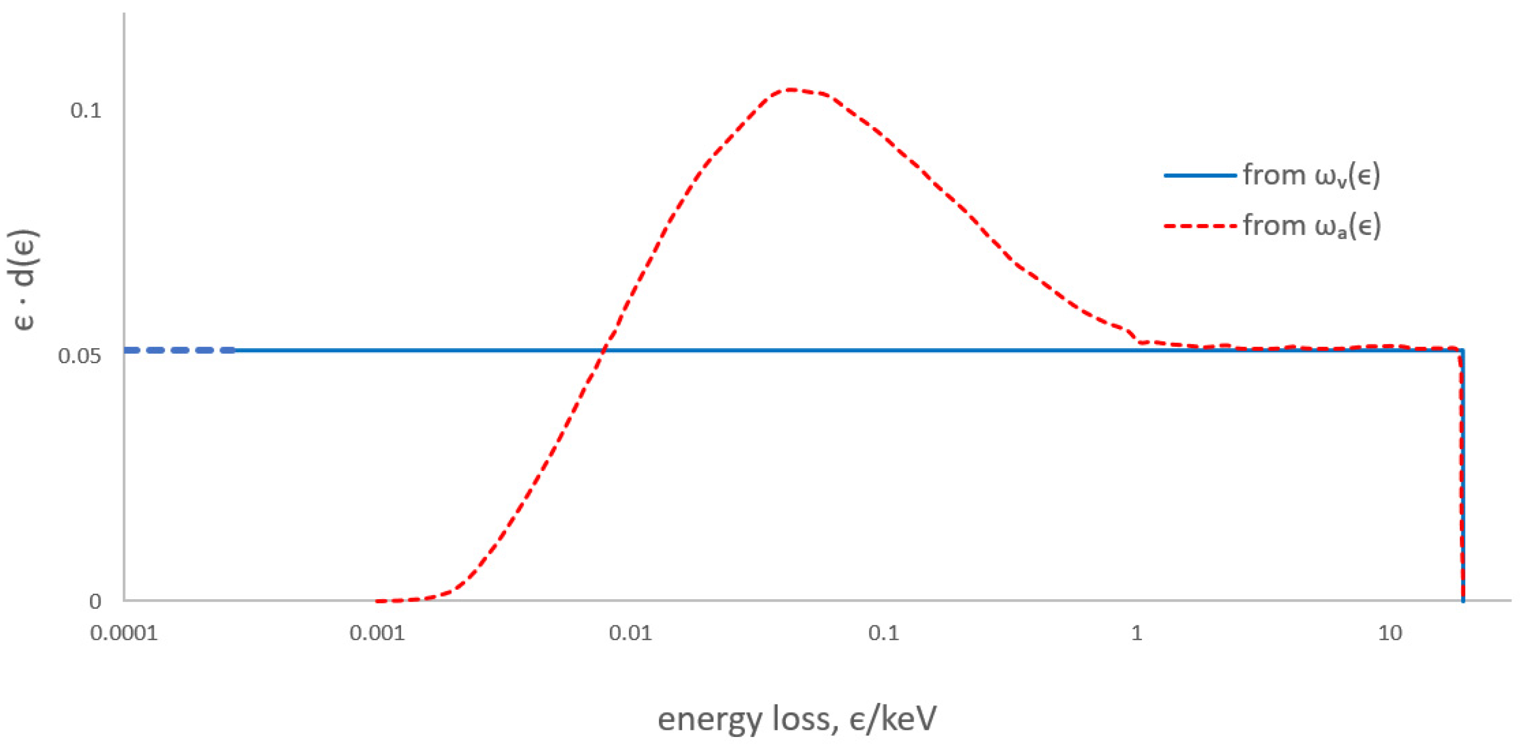
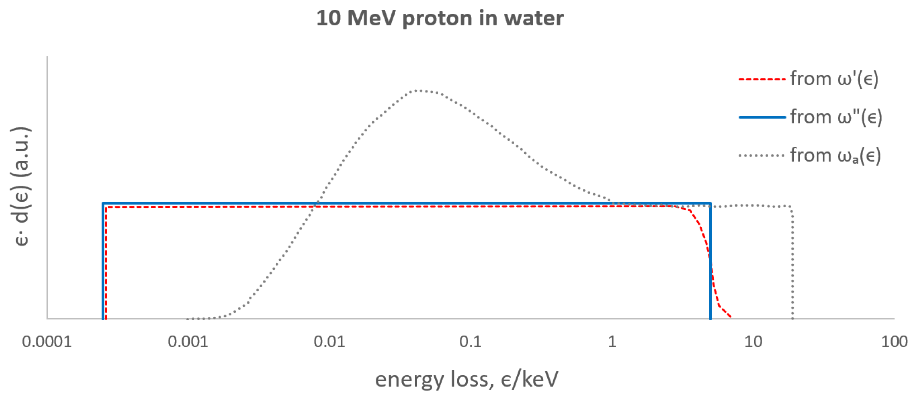
2.1.5. From Energy Loss to Energy Imparted

Delta rays have large ranges and some of their energy is delivered outside the SV. Therefore, for high-energy beams, the imparted energy distribution, here referred to as f′(є), is significantly different from the energy loss distribution f(є). This section discusses the modifications of the collision distributions, ω′(є), necessary to take into account the delta-ray escape; the distribution of the imparted energy, f′(є), is obtained by repeating the auto-convolution of ω′(є) analogously to the process described in Section 2.1.3. The distribution f′(є) refers only to events with energy deposits due to primary particles. Events due exclusively to delta rays generated outside the SV are currently ignored; however, these are experimentally significant, especially for high beam energies and can alter the distribution, as discussed in Section 3.3.
In theoretical microdosimetry, the angular distribution of the delta rays is usually not taken into account because the trajectories are expected to be isotropic. The same assumption is made in this investigation. Experimental investigations confirm that the trajectories of the delta rays are distributed over large solid angles; however, the emission is not isotropic. The direction normal to the beam axis is populated mainly by low and medium energy delta rays, while the direction parallel to the beam axis is mainly populated by high energy delta rays [17].
The probability of escape for delta rays is related to the size of the SVs in which they are generated. In detectors in the shape of a sphere, cube, or cylinder with a height equal to the base diameter, a single reference dimension is used to characterize the shape and, in turn, be related to the escape of the delta rays [18]. For slab detectors, the longitudinal and transverse dimensions can be different, sometimes drastically different, and this should be taken into account in relation to the delta ray escape. Solid-state microdosimeters used in ion beam therapy belong to this category; they are generally used by orienting the largest face perpendicular to the direction of the beam.

Escape-Modified Energy Distributions of Electronic Collisions

To account for the escape of the delta rays, the distribution ωb(є) should be changed to a new collision distribution ω′(є). Let us focus on the escape of delta rays and their effect at higher energies of the collision distribution. For high-energy beams, some delta rays have a much larger range than the size of the SV and escape is certain. For instance, the range in silicon of a 400 keV delta ray is 1 mm, as shown in Figure 4; the energy imparted by those delta rays into the SV of a few micrometers is only a small fraction of the total energy. On the other hand, delta rays with energies of the order of 1 keV have ranges less than 1 µm and a negligible probability of escaping the SV. It is realistic to think that the new distribution ω′(є) has a gradual decrease to zero with respect to the original distributions ωv(є) or ωa(є) in the region, where the range is comparable with the detector size. The dashed red line in Figure 5 illustrates the behavior of the energy-weighted escaped-modified distribution obtained from ω′(є).
In a more rigorous approach, Monte Carlo simulations should be used to take into account the emission angles of the delta rays, ranges, and collision position.

Simplification of the Escape-Modified Distributions

An approximate solution can be used to take into account the escape of the delta rays. Instead of the smooth transition of ω′(є) shown in Figure 5, the simplified collision distribution, ω″(є), is truncated to a chosen value of the energy єt, which is significant in terms of delta ray escape. Figure 5 shows the drastic simplification provided by choosing ω″(є) instead of ω′(є). For energies lower than 4 keV, ω″(є) coincides with the distribution ωb(є) discussed in Section 2.1.4. This approximation of a sharp cut is very similar to standard practice in cavity integrals for ion chambers using restricted stopping powers with an electron production cut. With a natural (and approximate) choice, it is assumed that єt corresponds to the energy having a range coinciding with half of the transversal dimension of the SV. The result is a rectangular distribution; the graphical comparison between the two distributions ω′(є) and ω″(є) (represented in terms of energy-weighted distributions) is shown in Figure 5 using a dashed red line and a solid blue line, respectively.
The distribution of the imparted energy f″(є) is evaluated by repeating the auto-convolution process that is described before in Section 2.1.3 for ω″(є).

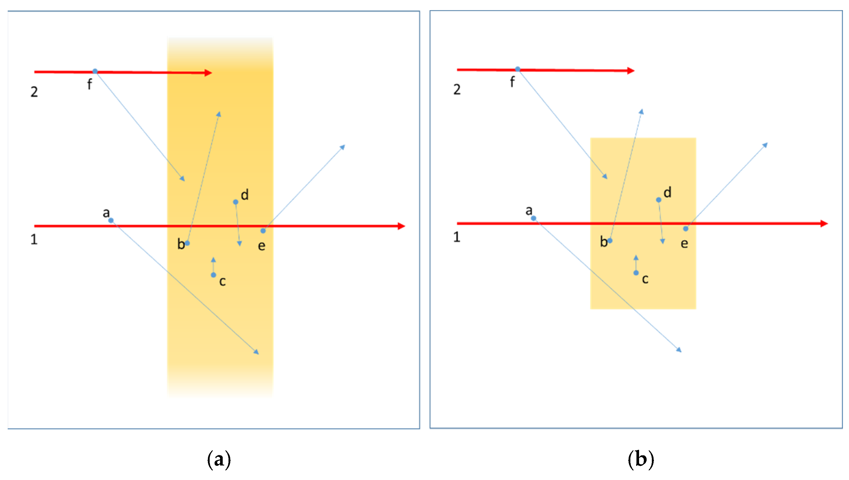
Further Considerations on the Energy Imparted and on the Escape of the Delta Rays

The energy imparted to the detector due to multiple collisions also depends on the transit of the delta rays inside and outside the walls of the SV. Two geometries are discussed, assuming that, in the region where the detector is positioned, the irradiation of the primary particles is uniform and unidirectional and the lineal energy transfer (LET) is constant.
Let us first focus on an ideal slab infinitely extended laterally so that the delta rays exit and re-enter only through the front and rear faces, see Figure 6a. Those delta rays that enter the SV are generated by the same primary particle that passes through the SV and are almost simultaneous. The energy subtracted from the escape of the delta rays is compensated, stochastically, by the inflow of energy due to the external delta rays. Perfect equilibrium occurs only when the radiation field is uniform and the wall effects in the microdosimeter are negligible. The latter condition is satisfied only if the material and the density of the SV are the same surrounding material. For solid-state microdosimeters, this condition is only approximate; while the back wall and the side walls are of the same material, often the front face of the microdosimeter is free or sealed with a layer of plastic materials. Since the number of primary events has not changed, the average energy per event of primary particles, ϵ ¯ 1 , is also unchanged. However, the profile of the imparted energy distribution is actually influenced by the transit of delta rays. What is expected is the decrease of events at highest energies compensated by the increase of events at lowest energies.
In the second case, a plate with limited lateral extension is considered in which the conditions of equilibrium of particles and energy are satisfied, see Figure 6b.
In this case, part of the energy is imparted by the delta rays which are generated by primary particles which do not cross the SV. Moreover, in this case, the equilibrium between the energy ejected and injected into the volume by the delta rays is also stochastically maintained. However, delta rays that are not synchronized with any primary event in the detector generate new events (represented by the delta ray “f” in Figure 6b). The total number of events is then increased. This corresponds to a decrease in the average energy deposited per event ϵ ¯ 1 . Events due solely to delta rays populate the lowest energy part of the spectrum. In the scanned ion beams, local irradiation inhomogeneity is likely to occur particularly at the boundary of the irradiated volume. If this happens, there is no equilibrium of particles or energy, and the number of primary and secondary particles may be non-uniform in space.

2.2. Method: Numerical Evaluations

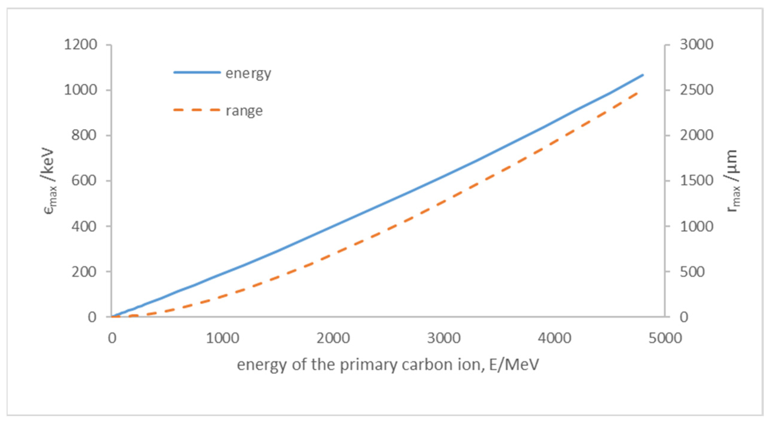
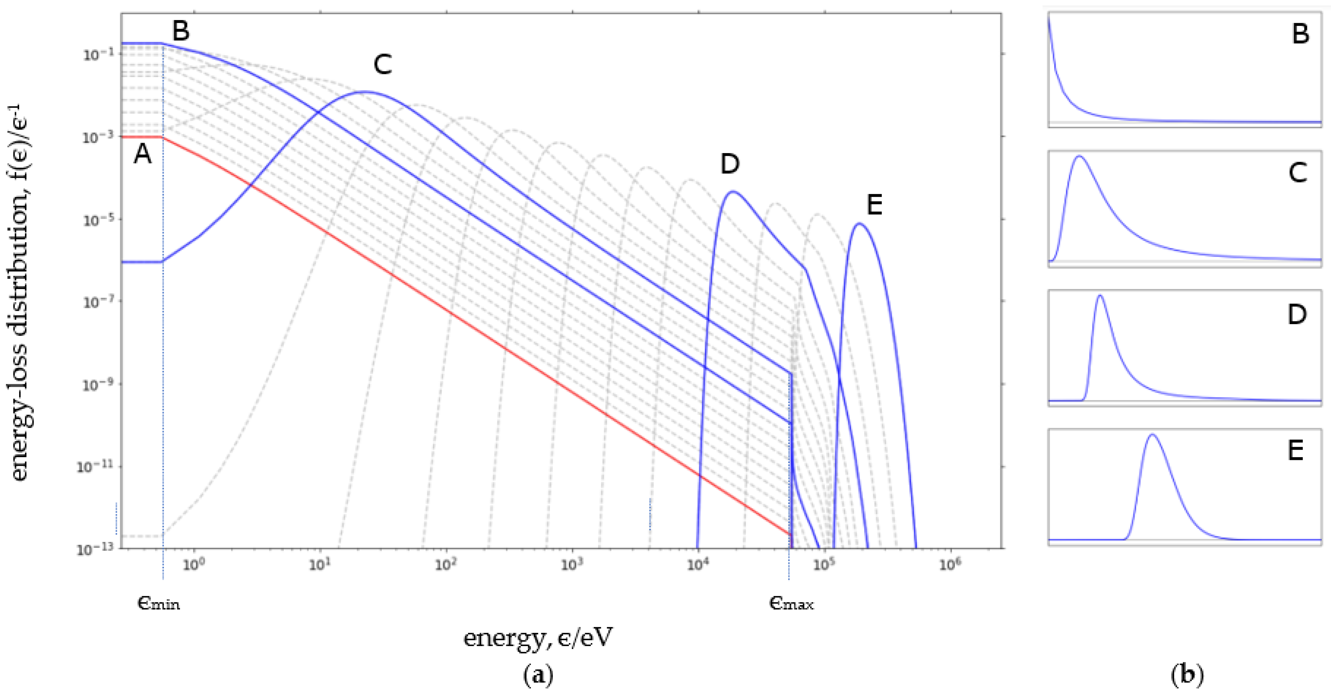
2.2.1. Electronic Collision Distribution

For the numerical evaluation, the exact representation of the probability density function of energy losses in the individual collisions must be replaced by a discrete distribution. The distribution ωb(є), corrected and simplified to take into account the binding energy of the electrons as discussed above, is replaced by its representation in discrete values ωb,i. This process is based on the following considerations:
  • The maximum value єmax is obtained as a result of the formula for the relativistic solution in Equation (4), considering the energy of the primary ion;
  • The value of єmin used in the discrete distribution is obtained using the approximate process according to Equation (14). This ensures that the calculated energy transferred per unit length matches the values provided by the selected electronic stopping power tables. The probability of collision in the interval 0 < є < єmin is given by the value P(0);
  • The energy increment Δi, in the discrete representation of ωb,i, is chosen to be constant and equal to єmin;
  • The value of δ1 calculated using the discrete sum:
    δ 1 = ϵ min є max ϵ i · ω b , i · i ,
  • must be equal to the exact solution calculated with Equation (3). To ensure this, the value of ωb,i for the i-th bin is not calculated at the edge of the bin (єi or єi+1) but at a point within the interval (єi, єi+1) at a distance ∂є. Therefore, the discrete values, ωb,i, approximating the analytic function, ωb(є), are obtained as:
    ω b , i = ω b ( є i   + є ) .
  • The value of ∂є is chosen as the value that equals the values of δ1 calculated numerically and exactly:
    δ 1 = ϵ min є max ϵ i · ω b ( є i + є ) · є min = ϵ min є max ϵ · ω b ( ϵ )   d ϵ ,
  • where ωbi + ∂є) = 1/(єi + ∂є)2 and, from Equation (1), ωb(є) = k02 in the interval of energies (єminmax). Therefore,
    є min · ϵ min є max ϵ i ( є i + є ) 2 = k 0 ( ln ϵ max ln ϵ min ) .
  • The discrete distribution is normalized also taking into account the value ωb,0 which refers to the condition of no collision. Therefore:
    0 є max ω b , i · i = 1 .

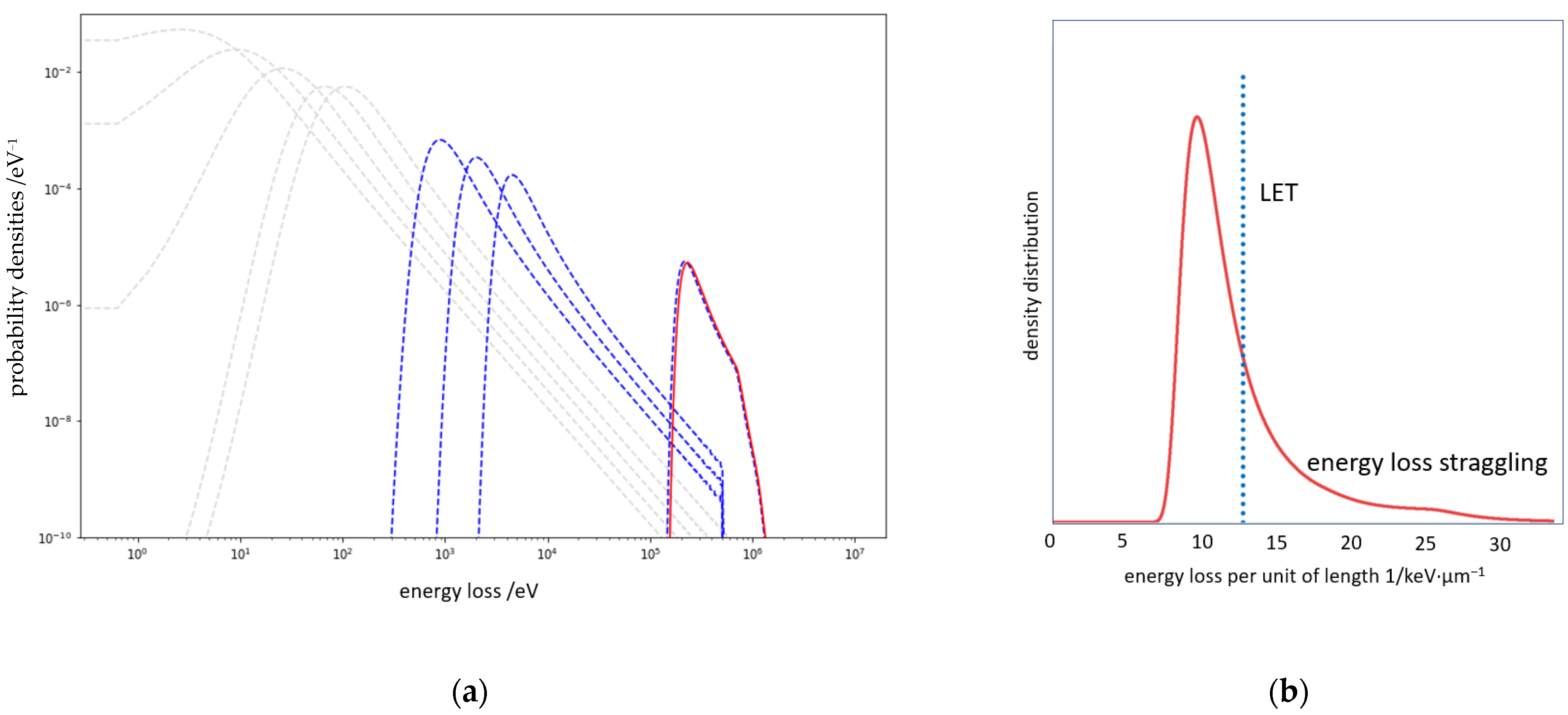
2.2.2. Energy-Loss Distribution

Once the energy limits of the discrete distribution (єmin and єmax), the values of the discrete distribution (ωb,i), the increment (Di), and the displacement (∂є) have been defined, the discrete distribution of energy loss fii) is evaluated by the numerical convolution process described in Equation (10). The mean energy lost in a thickness corresponding, on average, to µ collisions is ϵ ¯ = µ·δ1. This also corresponds to the first moment of the energy-loss distribution in Equation (3). Under typical microdosimetric conditions, the number of collisions, µ, is of the order of tens of thousands. The total number of bins in which the distribution is represented, corresponding to the ratio єmaxmin, can reach one million at the highest energies. To limit the computation time, care must be taken when setting the precision parameters for the convolutions.
Let us first take into account the energy lost in the electronic collision which is represented by a discrete distribution, (ωb,0, ωb,1, … ωb,i, …), which approximates the continuous distribution ωb(є). The energy loss straggling for thicknesses that double at each step is represented by the successive convolutions calculated using Equations (9) and (10). An example of the numerical convolutions representing energy loss straggling at various thicknesses is shown in Figure 7 for a 25 MeV·u−1 carbon ion beam in a silicon SV (єmin = 0.55 eV and єmax = 55.4 keV).
The curve f(є,d0) is indicated in the figure as (A) and all the first nine auto-convolutions show the trend of Rutherford’s cross-section, i.e., proportional to 1/є2. The distribution (B), after ten auto-convolutions, refers to the thickness corresponding, on average, to a single primary collision. By increasing the thickness of the SV, the probability of “non-collision” decreases and progressively, a peak is formed as in distribution (C). The spectra show a decline that occurs at approximately the value єmax, with a very slight dependence on the order of the auto-convolutions. For the distribution (C), κ is of the order of 10−3, and the distribution can be considered as a typical Landau distribution since the ratio between the values of the distribution at the peak and the fall is greater than 106. Continuing with the convolutions, this ratio progressively decreases. For the distribution (D), the peak amplitude is only one hundred times larger than the amplitude at the fall. The parameter κ assumes a value of the order of 0.2 and the truncation in the Landau distribution begins to be visible also in the linear representation. As the thickness further increases, the peak gradually shifts to the right side, reaching and exceeding єmax. For the distribution (E), the parameter κ is above unity and the profile approximates a Gaussian distribution.
In thicker detectors, when κ ≥ 10, the numerical solution based on convolutions can be replaced with an approximated analytical solution in the Gaussian form evaluated according to Seltzer and Berger [9] as:
f ( ϵ ) 1 ξ 2 π κ ( 1 β 2 / 2 ) e [ ( ϵ ϵ ¯ ) 2 2   κ ξ 2 ( 1 β / 2 ) ]
  • where the variance is given by σ 2 = ξ 2 κ ( 1 β 2 / 2 ) .

2.2.3. Energy-Imparted Distribution

Let us consider the case of a slab detector with limited lateral extension (a few tens of micrometers) for which the escape of delta rays must be taken into account to evaluate the distribution of energy imparted. Using the simplification described in Section 2.1.5, the effect of the delta-ray escape results in the new distribution ω″(є) obtained by estimating the appropriate threshold energy єt. The values of the elements ω″i coincide with the values of the elements ωb,i in the interval єmin ≤ є ≤ єt and are zero for є > єt. The discrete distribution of ω″i is used for the estimation of the imparted energy distribution. Obviously, the normalization is lost and sum of all ω″i is less than one. The first moment δ1″ is obtained by using the elements ω″i in Equation (19). On average, the ratio between the total energy imparted (µ·δ1″) and total energy loss (µ·δb,1) is independent of the thickness of the SV and it is simply given by (δ1″/δb,1).
Similarly to what is described in Section 2.1.5, the imparted energy distribution f″i(є) is obtained from successive convolutions of the modified collision distribution ω″i.
The effect of different threshold energies єt on the distribution f″i(є) is displayed in Figure 8. By decreasing the value of єt, the energy-imparted distributions rapidly approach a Gaussian distribution as the number of collisions increases. In the energy loss distribution, the long tail remains visible also for thicknesses corresponding, on average, to more than one thousand primary collisions.
As the energy of the primary particles decreases, єmax also decreases, and, in turn, the range of the delta rays decreases and approaches the size of the microdosimeter. At the same time, the number of primary collisions per unit of length increases. The lower the energy of the primary particle, the more the distribution profile resembles a Gaussian distribution.

2.3. Material: The Ion Beam and the Microdosimeter

Microdosimetric spectra were collected at the MedAustron ion therapy center using a silicon microdosimeter and carbon ion beams of nominal energy 213.4 MeV·u−1 and 284.7 MeV·u−1. The silicon microdosimeters used in this work are based on the concept of high-resistivity p-type silicon on insulator (p-SOI) and were developed at the Center for Medical Radiation Physics (CMRP) of the University of Wollongong, Australia [19,20]. The SV of the microdosimeter used in this investigation has a thickness of 10 µm and a circular cross-section with a diameter of 30 µm. A fixed (non-scanned) pencil beam with a quasi-Gaussian profile in both transversal directions and full width at half maximum of 6 mm is directed toward the center of the detector. Before reaching the microdosimeter, the beam passes through a layer of RW3 polystyrene with a water-equivalent thickness of 4.5 mm. The effect is a degradation of the nominal ion energies which results, according to the ICRU reference tables [21], in 207.8 MeV·u−1 and 279.8 MeV·u−1, respectively. According to SRIM reference tables [22], the resulting energies are 207.7 MeV·u−1 and 279.9 MeV·u−1, respectively. The relative energy uncertainty of the beam is assumed to be 1% of the energy. It is important to note that, in the context of ion beam therapy, the study of monoenergetic beams is not a limit when passive systems are also used to spread out the energy. Indeed, more recent systems are characterized by beams that are actively scanned in three dimensions and the complex irradiation of tumors can be broken down into individual contributions from monoenergetic beams.
The signal from the detector is first processed with the charge-preamplifier and a shaping amplifier made at Wollongong University and incorporated into the microdosimeter holder, producing a bipolar pulse with a shaping time of 3 µs. The shaped pulses are directed to the multi-channel analyzer of the company ORTEC, model 928 MCB, and processed using ORTEC’s Maestro software. Standard procedures for linearity corrections of the electronic chain are followed [23]. Calibration is performed based on the ion-edge method [24,25,26] using the ICRU tables [21] as a reference and correcting the maximum reference value of the electronic stopping power for the thickness of 10 µm of silicon [23]. The count rate is maintained between 1200 and 5700 counts per second to minimize the probability of pulse pile-up. The electronic noise spectra are collected before and after the irradiation; the noise distribution is assumed to be Gaussian and centered at zero and shows a five-standard-deviation width corresponding to 0.8 keV·µm−1.

3. Results

3.1. Energy-Loss Distribution

For the specified mono-energetic ion-beam energy, material, and thickness, the values of єmax, bmin and bmax, єmin, and dn/dx, are calculated from Equations (4), (11), (15) and (12), respectively. The value of the electronic stopping power, S is evaluated by linear interpolation of the tabulated values for carbon ions in silicon. The mean energy in the collisions between primary particle and electron of the medium δ1 and the mean number of collisions in the site μ are evaluated using Equations (11) and (12), respectively. Table 1 reports the collision parameters evaluated for a silicon microdosimeter with thickness of 10 µm.
Starting with f(є,d0), the distribution f(є,d1) is computed, according to Equation (10), as f(є,d1) = f(є,d0)⊗10. For the carbon ion energy of 207.8 MeV·u−1, a total of (1024·µ) = 35,450,880 convolutions of f(є,d0) should be performed. This number can be reduced to just 32 convolutions. In the procedure used to reduce the number of convolutions, it is useful to consider the number (1024·µ/2) and use its binary representation: 1 0000 1110 0111 1000 0000 0000. First, twenty-five auto-convolutions (corresponding to the number of binary digits) are recursively estimated. Then, the results of the 12th, 13th, 14th, 15th, 18th, 19th, 20th, and 25th convolutions (corresponding to the binary digits with value 1) are, in turn, convoluted; considering the properties of the auto-convolutions, an approximation can be made by excluding the convolutions below the 16th from this process, which would affect the final result by less than one-thousandth.
In the following, the use of the symbol y, which generally refers to lineal energy, is extended, in a somewhat arbitrary way, to the distributions of energy loss and to the distributions of energy imparted, indicating the energy loss per unit of length as yloss and the energy imparted per unit length as yimp.
Figure 9a represents on a logarithmic scale the sequence of convolutions relevant for the estimation of the density distribution of the energy loss. Figure 9b shows the result yloss of the convolution process for the 207.8 MeV·u−1 carbon ions traversing a 10-micrometer-thick silicon SV. This energy loss per unit length can be seen as the microdosimetric spectrum under the ideal circumstance that the delta-ray escape is negligible; it is given at density 1 g·cm−3 as it is done in general for lineal energy spectra [27]. As the value κ = 0.04 suggests, the distribution is represented by a truncated Landau function: the smooth truncation is visible in the figure at approximately 27 keV·µm−1.
For the primary particle energy of 279.8 MeV·u1, the required 28,765,184 convolutions are reduced to a total of 34 convolutions, 24 recursive auto-convolutions plus 10 additional convolutions (using the corresponding binary representation 1101 1011 0111 0110 0000 0000).

3.2. Energy-Imparted Distribution

To represent the imparted energy, the procedure based on recursive auto-convolutions described in Section 2.2.3 is performed starting from the modified collision distribution, ω″i.
The delta-ray escape is evaluated according to the procedure in Section 2.1.5 selecting as a threshold, єt, the energy of the electron whose range in silicon corresponds to the radius of the SV cross-section. For a silicon SV with a circular cross-section of 30 µm in diameter, the reference range is then 15 µm. Using ESTAR tables [16], this value of the range is obtained at the energy єt = 37.95 keV. The convolution process described in the previous section is repeated for the truncated collision distribution ω′i.
The result is shown in Figure 10 in terms of energy loss per unit length and energy imparted per unit length. The curves referring to the energy imparted use the normalization adopted for the energy loss. On the left side, until the peaks are reached, the two distributions are overlapping. The difference in the area under the curves represents the fraction of particles that are not accounted for because of the delta ray escape.

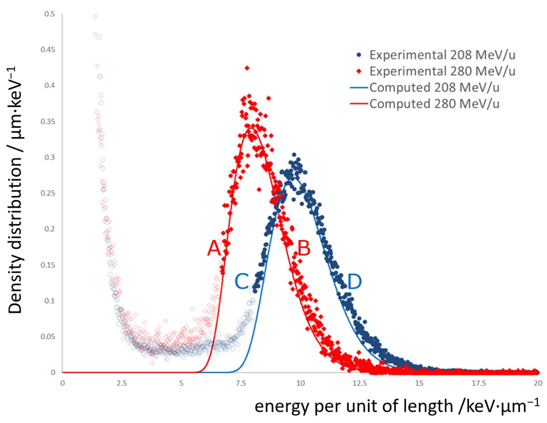
3.3. Comparison with Experimental Data

Microdosimetric spectra, collected at the energies of 207.8 MeV·u−1 and 279.8 MeV·u−1, are represented in Figure 11. The spectra are calibrated in lineal energy using the edge method described in the literature [24,25,26] and referring to the electronic stopping power tables for carbon ions in silicon from ICRU [21]. The imparted energy distribution evaluated according to Section 3.2 for the two carbon ion energies is also displayed in Figure 11. The microdosimetric spectra are reported in the less usual way, with f(y) as a function of lineal energy represented in linear scale, instead of the typical y·d(y) distributions in semi-logarithmic scale. In Figure 11, the values of the normalized spectrum are scaled by the factor b, with 0 < b < 1, to provide an overlap with the distribution of energy imparted per unit of length.
Experimental data show the dual role played by delta rays in the formation of a microdosimetric spectrum.
First, the escape of the delta rays determining the reduction of the tail at the highest energies, illustrated already in Figure 10a, is confirmed by the experimental data. In fact, there is a clear overlap between the calculated distributions with the experimental spectrum above point C for the energy of 207.8 MeV·u−1 and above the point A for the energy of 279.8 MeV·u−1.
Secondly, pulses due solely to delta rays populate the lower values of the spectrum, as shown in Figure 11 under points A and C in the two experimental curves. The ions responsible for the formation of this part of the spectrum are often referred to as “touchers” in microdosimetry.
For a monoenergetic beam and a known thickness of the detector, the rightmost part of the microdosimetric spectrum (above the point A and C in the two cases) are univocally correlated to the energy of the beam. Once the geometry of the SV and the beam energy are known, the energy loss distribution can be re-calculated numerically and, in this way, it is possible to indirectly evaluate the LET.
In the calibration of the distributions, the same electronic stopping power tables at the energies of 207.8 MeV·u−1 and 279.8 MeV·u−1 were used. The overlap of the experimental and computed peaks, shown in Figure 11, provides an indication of the correctness of the calibration and, in turn, of the consistency of the electronic stopping power values from the lookup tables with the experimental results over a broad energy span.
The profile of the imparted-energy distribution at the lowest values can be re-created starting from the experimental spectrum; for instance, for the spectrum referring to the energy of 207.8 MeV·u−1 in Figure 11, a quasi-Gaussian distribution interpolating the data in the interval A-B can be used to extrapolate the part below the point A (and similarly can be done for the 279.8 MeV·u−1 energy spectrum below the point C). This extrapolation can be used as a boundary line that divides those events where only delta ray energy is deposited, from the events in which the primary particles cross the sensitive volume. The spectra thus obtained provide an estimate of the relative fluency and relative dose contributions for the two different types of events.

3.4. Mean Values

The characterization in terms of radiation quality of the radiation fields is done often using the mean values either of lineal energy or of LET. The mean values of LET in track and dose are indicated as   L ¯ T and   L ¯ D , respectively. In the following discussion, the symbol y is used in relation to all the distributions discussed above; in particular, the energy loss per unit length is indicated as yloss and the energy imparted per unit length is indicated as yimp. The additional subscripts, ‘F’ and ‘D’, indicate the mean values calculated in frequency and dose, respectively. The beam is considered to be mono-energetic.

3.4.1. Mean Values of Energy Loss per Unit Length

In the distribution of the energy loss, the delta ray escape is not taken into account. As discussed in Section 2.1.4 and Section 2.2.1, the value of єmin is chosen precisely to ensure that the energy lost, per unit length, by the primary ions in electronic collisions coincides with the stopping power (see Equation (14)). Therefore, ȳloss,F, by construction, is equal to   L ¯ T . However, ȳloss,D is not a correct estimator of   L ¯ D , as can be deducted directly considering that, in the example, ȳloss,F < ȳloss,D while, being a monoenergetic beam,   L ¯ T =   L ¯ D . In the specific condition of no delta-ray escape, the difference between ȳloss,D and   L ¯ D can be quantified by expressing the relative variance of lineal energy, Vy,loss, as a function of all other relative variances as discussed by Kliauga et al. [28]:
V y , loss = V L + V + V · V L + V S + V exp
where VL refers to LET, V to the chord length, vs. to the energy-loss straggling, and Vexp to the experimental factors. No further discussion is provided here as to the source of these variances and how they relate to the radiation and detector characteristics; these can be found in the references cited. Considering an ideal mono-energetic beam, the variance of VL is zero. In the approximation that all ion tracks crossing a slab detector have the same length, the variance V is also negligible. Furthermore, since the energy loss distribution is purely computational, experimental uncertainty contributions should not be considered. Therefore, the only relative variance terms remaining in Equation (23) are Vy,loss and VS. The first can be represented as Vy,loss = (ȳloss,Dloss,F − 1) as can be deducted from the definition of the variance of the distribution. The second, as described by Kellerer [12], can be indicated as V S = δ 2 / ϵ ¯ where δ2 is the second moment of the collision distribution from Equation (3) and ϵ ¯ = δ1·μ is the mean energy lost in the SV. The correlation of variances in Equation (23) is then reduced to the equation:
V y , loss V S     y ¯ loss , D   y ¯ loss , F 1 δ 2 ϵ ¯ .
Therefore:
  y ¯ loss , D   y ¯ loss , F + δ 2 ϵ ¯ ϵ ¯ ¯ =   L ¯ D + δ 2 ¯ .
showing that, for a monoenergetic beam, ȳloss,D exceeds   L ¯ D by a non-negative factor.

3.4.2. Mean Values of Energy Imparted per Unit Length

Since the imparted-energy distribution is less populated by events in the high energy part and more populated in the low energy part, the value of ȳimp,F is less than the value ȳloss,F, and   L ¯ T . This result is general and can be extended to non-monoenergetic radiation. However, the result of this example ȳimp,D <   L ¯ D is not general.

3.4.3. Mean Values of Lineal Energy

As shown in Figure 11, the experimental microdosimetric spectrum overlaps the imparted-energy distributions per unit of length except for the presence of the low-energy tail. For this reason, the experimental mean values of lineal energy, ȳF and ȳD are lower than the corresponding values ȳimp,F and ȳimp,D.
Combining the above results, the correlations between the average frequency quantities are as follows:
  y ¯ F     y ¯ imp , F     y ¯ loss , F =   L ¯ T .
The validity is general, including non-monoenergetic radiation fields. For the dose-mean quantities, the condition ȳD ≤ ȳimp,D   L ¯ D   ≤ ȳloss,D shown in the example cannot be generalized. The correlations that are valid also for non-monoenergetic radiation fields are:
  y ¯ D     y ¯ imp , D     y ¯ loss , D   L ¯ D     y ¯ loss , D .
The experimental lineal energy spectrum cannot be represented below the noise cutoff level, c. The partial frequency and dose mean values are defined and normalized in the interval c ≤ y ≤ ∞. They are represented, respectively, by the integrals:
y ¯ F , c = c y · f ( y ) d y   , y ¯ D , c = c y · d ( y ) d y .
These values inevitably overestimate the noise-free mean values of the lineal energy which would extend over the full interval 0 ≤ y ≤ ∞.

3.4.4. Comparison of Mean Values

The mean values calculated for the distributions and the spectra discussed before are summarized, in the case of the 207.8 MeV·u−1 carbon-ion beam, in Table 2 and, in the case of the 279.8 MeV·u−1 carbon ion beam, in Table 3.
In these examples and from the consideration in Section 3.4.1Section 3.4.3, it is clear that, for a monoenergetic beam, the only numerical value which equals   L ¯ T and   L ¯ D is yloss,F.
The cutoff value c has a high relevance on the evaluation of the mean lineal energies. For example, for the spectrum of 207.8 MeV·u−1, assuming a value c = 8 keV·µm−1, the ȳc,F and ȳc,D result in 10.30 keV·µm−1 and 10.48 keV·µm−1 respectively, rather close to the homologous values of the imparted energy. Similarly, assuming for the spectrum of 279.8 MeV·u−1 the cutoff c = 6 keV·µm−1, the values of ȳc,F and ȳc,D become 8.44 keV·µm−1 and 8.65 keV·µm−1, respectively.

4. Discussion

This work studies energy straggling and delta ray escape for carbon ion beams and their correlations with the SV geometry of microdosimetric detectors. For two energies, 279.8 MeV·u−1 and 207.8 MeV·u−1, the distributions of energy loss per unit of length and energy imparted per unit length are computed numerically considering the effects of the energy loss straggling and the delta-ray escape. Excluding the lowest part of the spectrum, which is related to the energy imparted from the delta rays generated outside the SV, the comparison of the evaluated and the experimental spectra shows a satisfactory agreement.
At the highest values of the spectrum, the profile of the distribution of the energy imparted per unit of length is obtained excluding the contribution of those delta rays whose range exceeds the transverse radius of the SV. Although simplistic, this is a satisfactory choice as confirmed by the agreement between the computed and experimental data. This choice, being based on the geometry of the SV, does not require any free parameters in the computations and this is an added advantage. However, more sophisticated evaluations of delta-ray escape can be performed which may provide a better agreement between the distributions.
At the lowest values of the spectrum, the tail due to the delta rays generated outside the SV is a source of distortions. The problem arises from the impossibility of determining, below the threshold due to the electronic noise, the profiles of the experimental spectrum which is largely populated of events deriving from the delta rays. To overcome this problem partially, a mitigation strategy is proposed in the outlook section below.
It is important to consider two uses of microdosimetry that are proposed in the context of ion beam therapy.
First, the microdosimeters as seen as tools that provide the experimental base for the determination of   L ¯ F and   Ly ¯ D . This investigation provides, for that aspect, somewhat conclusive results for middle and high energies monoenergetic beams. In fact, as shown comparing Figure 10 and Figure 11, the interval of the experimental spectrum between the point A and the peak for the beam energy of 279.8 keV·µm−1 (and analogously the experimental spectrum between the point C and the peak for the beam energy of 207.8 keV·µm−1) can be used to univocally identify the ion-beam energy; as long as the irradiation penetrating the target can be considered as monoenergetic, the value of the energy identifies univocally the mean LET values. However, these results cannot be extended to the case of non- monoenergetic beams or for microdosimetric spectra collected in the Bragg peak.
The second use considers microdosimeters as the tools that provide the most complete characterization of the different radiation qualities of the therapeutic ion beams. This study provides a computational method to distinguish two components of the spectrum of a mixed radiation field, the partial spectrum due exclusively to delta rays and the partial spectrum due to primary ions.

4.1. LET Estimation

The lineal energy spectra and mean values, collected using microdosimeters with SVs of the order of the cell’s nucleus size, are representative of the energy interaction of the ionizing particles with a biological target.
The fact that the values of ȳF and ȳD are different from the respective values   L ¯ T and   L ¯ D is well known and reported in literature. Empirical multiplication factors, which depend on the shape of the SV but not on the energy of the primary ions, were used to compensate for the discrepancies between the values of ȳF and ȳD and the values of   L ¯ T and   L ¯ D , respectively. This study showed how the microdosimetric spectra are the complex result of events due to delta rays and primary ions and how these contributions vary with the energy of the beam; the use of the simple empirical multiplication factor therefore seems to be an oversimplification.
The evaluation of the lineal energy mean values is highly dependent on the cutoff limit imposed by the electromagnetic noise on the microdosimetric spectra. An example illustrates how the evaluation of ȳF and ȳD, moving the noise cutoff value from 0.8 keV·µm−1 to 6 keV·µm−1, results to an increase of ȳF by 85% and of ȳD by 16%. This is a critical point since different solid-state detectors have very different noise cutoff values and this inevitably leads to large discrepancies. Additionally, the study shows how the role played by the energy carried out by the escaping delta ray and by the energy injected from external delta rays is rather complex and evolves with the ion energy and the size of the SV.
It is expected that, by progressively decreasing the energy of the beam, the fraction of the escaping delta rays is reduced and, consequently, the distribution of the energy imparted is more similar to the distribution of energy losses. In the experimental spectrum, the tail at low lineal energies becomes less pronounced. Gradually, the number of primary collisions per unit of length increases and the spectrum approaches a Gaussian distribution whose full width at half maximum becomes, in relative terms, narrower and narrower. Under these conditions, the average frequency value of the lineal energy ȳF approximates   L ¯ T (and ȳD approximates   L ¯ D ).
The discrepancies between microdosimetric-based and LET-based parameters are less important if the overall radiation of the clinical target is considered. In fact, in typical treatment sessions, the mitigation effects due to the use of multiple portals and the variety of particle energies that contribute to the planned dose of the tumor target must be taken into account. Virtually all the target subvolumes are irradiated, at least partially, with the low-energy radiation of the Bragg peak region where LET and lineal energy are comparable.

4.2. Outlook

This investigation is part of a more extensive study on the characterization of therapeutic ion beams in terms of lineal energy [23] and these topics will be the subject of future analysis. Computational evaluation of energy loss straggling and the delta-ray escape is an important element for the quantitative re-consideration of several topics discussed since microdosimetry began investigating therapeutic ion beams with solid-state detectors.
Some methods have been proposed to reconstruct the part of the spectrum below the noise cutoff using extrapolations. For the beam energies comparable with those considered in this investigation, a computational procedure can be used instead to integrate the missing information of the dose distribution d(y). Under the assumption of energy equilibrium, the area under the two energy-weighted distributions of the energy loss and the experimental energy imparted, d(є), is the same. Therefore, the excess area of the energy loss distribution at the highest values of the spectra must be compensated by an equal area in the lower part where the energy-weighted experimental spectrum exceeds the energy-weighted energy-loss distribution. A rigorous analysis is needed that takes into account the impact of all the terms including the effects of the simplification in the delta-ray escape, the limits of the assumption of energy equilibrium, and the impact of the increase of the number of events in frequency spectra due to the influx of delta rays. Furthermore, an analytical approach could be envisaged for calculating the spectrum of the injected electron slowing down. All these investigations go beyond the scope of this work and are the subject of subsequent systematic studies.

Author Contributions

Conceptualization, G.M. and H.P.; methodology, G.M.; software, G.M.; validation, G.M.; formal analysis, G.M.; investigation, C.M., S.B. and G.M.; resources, A.R.; data curation, G.M.; writing—original draft preparation, G.M. and H.P.; writing—review and editing, G.M., H.P., S.B., A.R. and C.M. All authors have read and agreed to the published version of the manuscript.

Funding

The work of S.B. in this research was funded by the Austrian Science Fund through project number P32103-B.

Institutional Review Board Statement

Not applicable.

Informed Consent Statement

Not applicable.

Data Availability Statement

Data presented in this article is available on request from the corresponding author.

Conflicts of Interest

The authors declare no conflict of interest.

References

  1. Rossi, H.H. Specification of Radiation Quality. Radiat. Res. 1959, 10, 522–531. [Google Scholar] [CrossRef] [PubMed]
  2. Kellerer, A.M. Microdosimetry and the theory of straggling. In Biophysical Aspects of Radiation Quality, Second Panel Report; International Atomic Energy Agency: Vienna, Austria, 1968; pp. 89–104. ISBN 92-0-011068-1. [Google Scholar]
  3. Rutherford, E. The scattering of α and β particles by matter and the structure of the atom. Lond. Edinb. Dublin Philos. Mag. J. Sci. 1911, 21, 669–688. [Google Scholar] [CrossRef]
  4. Landau, L. On the energy loss of fast particles by ionization. J. Phys. (USSR) 1944, 8, 201–205. [Google Scholar]
  5. Bohr, N. The Penetration of Atomic Particles through Matter; Matematisk-fysiske Meddelelser; Royal Danish Academy of Sciences and Letters: Copenhagen, Denmark, 1948; Volume 18, No. 8, pp. 63–73. [Google Scholar]
  6. Vavilov, P.V. Ionization losses of high-energy heavy particles. Soviet Phys. JETP 1957, 5, 749–751. [Google Scholar]
  7. Bichsel, H. Straggling and particle identification in silicon detectors. Nucl. Instrum. Meth. A 1970, 78, 277–284. [Google Scholar] [CrossRef] [Green Version]
  8. Bichsel, H. Energy loss and ionization of fast charged particles in a 20 μm silicon detector. Nucl. Instrum. Meth. A 1985, 235, 174. [Google Scholar] [CrossRef]
  9. Seltzer, M.; Berger, M.J. Energy loss straggling of protons and mesons. In Studies in Penetration of Charged Particles in Matter; Nuclear Science Series 39; National Academy of Sciences: Washington, DC, USA, 1964. [Google Scholar]
  10. Hancock, S.; James, F.; Movchet, J.; Rancoita, P.G.; VanRossum, L. Energy loss and energy straggling of protons and pions in the momentum range 0.7 to 115 GeV/c. Phys. Rev. A 1983, 28, 615–620. [Google Scholar] [CrossRef] [Green Version]
  11. Kellerer, A.M. Calculation of Energy Deposition Spectra. In Report of Panel on Biophysical Aspects of Radiation Quality; International Atomic Energy Agency: Vienna, Austria, 1968; pp. 57–74. [Google Scholar]
  12. Kellerer, A.M. Fundamentals of Microdosimetry. In The Dosimetry of Ionizing Radiation; Kase, K.R., Bjärngard, B.E., Attix, F.H., Eds.; Academic Press, Inc.: Cambridge, MA, USA, 1985; Volume I. [Google Scholar]
  13. Bohr, N., II. On the theory of the decrease of velocity of moving electrified particles on passing through matter. Lond. Edinb. Dublin Philos. Mag. J. Sci. 1913, 25, 10–31. [Google Scholar] [CrossRef]
  14. Bolst, D.; Guatelli, S.; Tran, L.T.; Rosenfeld, A.B. The impact of sensitive volume thickness for silicon on insulator microdosimeters in hadron therapy. Phys. Med. Biol. 2020, 65, 035004. [Google Scholar] [CrossRef] [PubMed]
  15. Verona, C.; Cirrone, G.A.P.; Magrin, G.; Marinelli, M.; Palomba, S.; Petringa, G.; Verona Rinati, G. Microdosimetric measurements of a monoenergetic and modulated Bragg Peaks of 62 MeV therapeutic proton beam with a synthetic single crystal diamond microdosimeter. Med. Phys. 2020, 47, 5791–5801. [Google Scholar] [CrossRef] [PubMed]
  16. Berger, M.J.; Coursey, J.S.; Zucker, M.A.; Chang, J. NIST Standard Reference Database 124: Stopping-Power & Range Tables for Electrons, Protons, and Helium Ions. Available online: http://physics.nist.gov/Star (accessed on 2 March 2022).
  17. Booz, J.; Braby, L.; Coyne, J.; Kliauga, P.; Lindborg, L.; Menzel, H.-G.; Parmentier, N. ICRU Report 36, Microdosimetry. J. Int. Comm. Radiat. Units Meas. 1983, os19, r1983. [Google Scholar] [CrossRef]
  18. Kellerer, A.M. Criteria for the Equivalence of Spherical and Cylindrical Proportional Counters in Microdosimetry. Radiat. Res. 1981, 86, 277–286. [Google Scholar] [CrossRef] [Green Version]
  19. Tran, L.T.; Prokopovich, D.A.; Petasecca, M.; Lerch, M.L.; Kok, A.; Summanwar, A.; Hansen, T.E.; Da Via, C.; Reinhard, M.I.; Rosenfeld, A.B. 3D radiation detectors: Charge collection characterisation and applicability of technology for microdosimetry. IEEE Trans. Nucl. Sci. 2014, 61, 1537–1543. [Google Scholar] [CrossRef] [Green Version]
  20. Tran, L.T.; Chartier, L.; Prokopovich, D.A.; Bolst, D.; Povoli, M.; Summanwar, A.; Kok, A.; Pogossov, A.; Petasecca, M.; Guatelli, S.; et al. Thin Silicon Microdosimeter Utilizing 3-D MEMS Fabrication Technology: Charge Collection Study and Its Application in Mixed Radiation Fields. IEEE Trans. Nucl. Sci. 2018, 65, 467–472. [Google Scholar] [CrossRef] [Green Version]
  21. Bimbot, R.; Geissel, H.; Paul, H.; Schinner, A.; Sigmund, P.; Wambersie, A.; Deluca, P.; Seltzer, S.M. ICRU Report 73, Stopping of Ions Heavier Than Helium. J. Int. Comm. Radiat. Units Meas. 2005, 5, i-253. [Google Scholar] [CrossRef]
  22. Ziegler, J.F.; Ziegler, M.D.; Biersack, J.P. SRIM—The stopping and range of ions in matter. Nucl. Inst. Methods Phys. Res. B 2010, 268, 1818–1823. [Google Scholar] [CrossRef] [Green Version]
  23. Meouchi, C.; Barna, S.; Puchalska, M.; Tran, L.; Rosenfeld, A.; Verona, C.; Verona-Rinati, G.; Palmans, H.; Magrin, G. On the measurement uncertainty of microdosimetric quantities using diamond and silicon microdosimeters in carbon-ion beams. Med. Phys. 2022; in press. [Google Scholar]
  24. Conte, V.; Moro, D.; Grosswendt, B.; Colautti, P. Lineal energy calibration of mini tissue-equivalent gas-proportional counters (TEPC). In Proceedings of the AIP Conference Proceedings, Timisoara, Romania, 21–24 November 2013; Volume 1530, pp. 171–178. [Google Scholar]
  25. Parisi, A.; Boogers, E.; Struelens, L.; Vanhavere, F. Uncertainty budget assessment for the calibration of a silicon microdosimeter using the proton edge technique. Nucl. Inst. Methods Phys. Res. A 2020, 978, 164449. [Google Scholar] [CrossRef]
  26. Bianchi, A.; Mazzucconi, D.; Selva, A.; Colautti, P.; Parisi, A.; Vanhavere, F.; Reniers, B.; Conte, V. Lineal energy calibration of a mini-TEPC via the proton-edge technique. Radiat. Meas. 2021, 141, 106526. [Google Scholar] [CrossRef]
  27. Goodhead, D.T. Relationship of Microdosimetric Techniques to Applications in Biological Systems. In The Dosimetry of Ionizing Radiation; Kase, K.R., Bjärngard, B.E., Attix, F.H., Eds.; Academic Press: Cambridge, MA, USA, 1987; pp. 1–89. ISBN 9780124004023. [Google Scholar] [CrossRef]
  28. Kliauga, P.; Waker, A.J.; Barthe, J. Design of tissue equivalent proportional counters. Radiat. Prot. Dosim. 1995, 61, 309–322. [Google Scholar] [CrossRef]
Figure 1. Energy-weighted density distribution of energy loss in a 10 MeV proton–electron collision in a water target. The dashed red line is based on the modified distribution according to Kellerer ωa(є) [12]; it takes into account the electron binding energy and is normalized. The solid blue line is based on the distribution of Equation (1), ωV(є); in this representation, there is no lower limit of the collision energy and the amplitude is not normalized but adapted to match the modified distribution at higher values.
Jne 03 00008 g001
Figure 2. Mean energy of the delta rays produced in a single collision of the primary particle with the electrons of the medium. The dotted line corresponds to the W-value in silicon.
Jne 03 00008 g002
Figure 3. Value of the parameter κ/d (thick blue lines) and ξ/d (thin red lines) calculated for carbon ions in a silicon slab where d indicates the thickness of the SV in micrometers. The different backgrounds refer to the different conditions for which the energy straggling is well represented by a Landau distribution (darker blue), a truncated Landau distribution (medium blue), a quasi-Gaussian distribution (lighter blue), or a Gaussian distribution (white).
Jne 03 00008 g003
Figure 4. Maximum delta ray energy (from Equation (4)) and maximum delta rays CSDA range (calculated using the ESTAR tables [16]) for primary carbon ions in a silicon target.
Jne 03 00008 g004
Figure 5. Illustrative representation of the energy-weighted single collision distribution of, є·d(є) partially using Kellerer results [12]. The dashed red line corresponds to the ω′(є) distribution; the solid blue line corresponds to the simplified distribution ω″(є) used in this work to account for the binding energy of the electrons and the escape of the delta rays. To facilitate comparison, the distribution obtained from the modified Kellerer distribution, ωa(є), is also displayed with a gray dashed line.
Jne 03 00008 g005
Figure 6. Schematic representation of the energy imparted in two slabs with different transverse extensions (orange rectangles). The trajectories of the ions are indicated with the thick red arrows 1 and 2. The path of the delta rays is represented using thin blue arrows and the letters from a to f; no secondary delta rays are represented. (a) Slab with infinite lateral extension; the missing energy deposits due to the escape of the delta rays are stochastically compensated with the energy deposits of the delta rays generated outside. (b) Slabs with limited lateral extension; the energy deposits from delta rays generated by primary particles that do not cross the SV and are counted as new events (represented by the blue arrow f).
Jne 03 00008 g006
Figure 7. (a) The recursive convolutions of the discrete energy loss distribution calculated for 25 MeV·u−1 carbon ions in silicon. The curve (A) corresponds to f(є,d0) of Equation (9). All other distributions are represented with grey dashed lines corresponding to f(є,d0) convoluted a number of times increasing to the power of two. Some distributions, emphasized with solid blue lines correspond to the following: (B) energy loss distribution f(є,d1), corresponding, on average, to one electronic collision (µ = 1); (C) Landau-shaped distribution (µ = 24); (D) energy loss distribution (µ = 212) showing a truncation at values slightly higher than єmax; (E) energy loss distribution (µ = 215) showing a quasi-Gaussian behavior. (b) Distributions (B–E) represented in linear scale with arbitrary units.
Jne 03 00008 g007
Figure 8. Energy loss straggling distribution f′(є) for 300 MeV carbon ions in 4.5-micrometer silicon target (solid red line) and effects on the energy imparted distribution when the delta ray above the energy of 16.6 keV (dashed black line), 11.7 keV (dashed dark grey line), and 5.5 keV (dashed light grey line) are excluded.
Jne 03 00008 g008
Figure 9. (a) Logarithmic representation of the most significant auto-convolutions; the curves, with peaks moving from left to right, are the 12th, 13th, 14th, 15th (dashed light grey) 18th, 19th, 20th, 25th, and (dashed blue) auto-convolutions; the solid red curve represents the energy loss distribution in a 10-µm-thick silicon SV of 207.8 MeV·u−1 carbon ions. (b) The same distribution represented in linear scale and terms of energy loss per unit of length; for comparison, the corresponding value of LET is indicated (dotted blue line).
Jne 03 00008 g009
Figure 10. (a) Distribution of the energy loss (dashed red line) and energy imparted (blue solid line) by primary particles per unit of length calculated for 207.8 MeV/u carbon ion energy in silicon target with thickness of 10 µm and diameter of 30 µm. (b) Energy imparted per unit of length for the two beam energies of 207.8 MeV/u and 279.8 MeV/u; the data referring to energy imparted are calculated using a threshold for the delta-ray energy at 37.95 keV.
Jne 03 00008 g010
Figure 11. Comparison of the distributions of imparted energy per unit of length (showed in Figure 10b) of 207.8 MeV·u−1 (blue solid line) and 279.8 MeV·u−1 (red solid line) with the experimental microdosimetric spectra obtained for the carbon-ion energies of 207.8 MeV·u−1 (blue dots) and 279.8 MeV·u−1 (red dots) in a 10-µm-thick, 30-µm-diameter silicon microdosimeter. The letters A, B, C, and D identify particular points of the distribution useful for discussing the results. The experimental values below A for the 279.8 MeV·u−1 beam (and below C for the 207.8 MeV·u−1) are dimmed to emphasize the different ionization sources hypothesized in the text.
Jne 03 00008 g011
Table 1. Collision parameters for carbon ions on a silicon microdosimeter with thickness of 10 µm.
ParameterUnitCarbon Ions
279.8/MeV·u−1207.8/MeV·u−1
κ, (relativistic estimation) 2.23 × 10−23.82 × 10−2
ξ¸ approximation of the mean total energy lost, through electronic collisions,
in the detector
keV15.6919.34
єmax,
maximum delta-ray energy
(relativistic estimation)
eV7.04 × 1055.06 × 105
єmin,
minimum delta-ray energy
eV6.41 × 10−16.34 × 10⁻¹
δ1, mean collision energy
of the ion and electron
in the medium
eV8.91 8.62
dµ/dx, mean number of primary collisions per unit of length nm−12.813.461
µ, mean number of primary
collisions in the SV
2.81 × 1043.46 × 104
d1, mean distance between
primary collisions
nm3.56 × 10−12.89 × 10⁻¹
Sel/r, mass electronic stopping power from
ICRU lookup tables [21]
keV·µm−110.7912.86
Sel/r, mass electronic stopping power from
SRIM lookup tables [22]
keV·µm−110.4312.45
Table 2. Track-average and dose-average LET, frequency-mean and dose mean lineal energy for experimental spectra, energy-imparted distributions, and energy loss distributions referring to a 207.8 MeV/u carbon-ion beam in the silicon slab microdosimeter.
y ¯ F
(keV·μm−1)
ȳ D (keV·μm−1) L ¯ T (keV·μm−1) L ¯ D (keV·μm−1) L ¯ T / ȳ F L ¯ D / ȳ D
LET 1 12.8512.85
ya, 24.938.82 2.611.46
yimp, 310.3110.46 1.251.23
yloss,12.8314.49 10.89
1 from ICRU stopping power table. 2 above the cutoff c = 0.8 keV·µm−1. 3 renormalized after excluding delta rays with energies above 35 keV.
Table 3. Track-average and dose-average LET, frequency-mean and dose-mean lineal energy for experimental spectra, energy imparted distributions, and energy loss distributions referring to a 279.8 MeV/u carbon-ion beam in the silicon slab microdosimeter.
ȳF
(keV·µm−1)
ȳD
(keV·µm−1)
L ¯ T (keV·μm−1) L ¯ D (keV·μm−1) L ¯ T / ȳ F L ¯ D / ȳ D
LET 1 10.7910.79
yc, 24.557.46 2.371.44
yimp, 38.458.60 1.281.25
yloss,10.7813.05 10.83
1 from ICRU Stopping power table. 2 above the cutoff c = 0.8 keV·µm−1. 3 renormalized after excluding delta rays with energies above 35 keV.
Publisher’s Note: MDPI stays neutral with regard to jurisdictional claims in published maps and institutional affiliations.

