Article

Similarity of Musical Timbres Using FFT-Acoustic Descriptor Analysis and Machine Learning

Center of Mathematics, Computer Science, and Cognition, Federal University of ABC, Av. Dos Estados, 5001, Santo André 09210-580, SP, Brazil
*
Author to whom correspondence should be addressed.
Eng 2023, 4(1), 555-568; https://doi.org/10.3390/eng4010033
Submission received: 25 December 2022 / Revised: 4 February 2023 / Accepted: 6 February 2023 / Published: 9 February 2023
(This article belongs to the Special Issue Feature Papers in Eng 2022)

Abstract

:
Musical timbre is a phenomenon of auditory perception that allows the recognition of musical sounds. The recognition of musical timbre is a challenging task because the timbre of a musical instrument or sound source is a complex and multifaceted phenomenon that is influenced by a variety of factors, including the physical properties of the instrument or sound source, the way it is played or produced, and the recording and processing techniques used. In this paper, we explore an abstract space with 7 dimensions formed by the fundamental frequency and FFT-Acoustic Descriptors in 240 monophonic sounds from the Tinysol and Good-Sounds databases, corresponding to the fourth octave of the transverse flute and clarinet. This approach allows us to unequivocally define a collection of points and, therefore, a timbral space (Category Theory) that allows different sounds of any type of musical instrument with its respective dynamics to be represented as a single characteristic vector. The geometric distance would allow studying the timbral similarity between audios of different sounds and instruments or between different musical dynamics and datasets. Additionally, a Machine-Learning algorithm that evaluates timbral similarities through Euclidean distances in the abstract space of 7 dimensions was proposed. We conclude that the study of timbral similarity through geometric distances allowed us to distinguish between audio categories of different sounds and musical instruments, between the same type of sound and an instrument with different relative dynamics, and between different datasets.

1. Introduction

Musical timbre is a multidimensional attribute of musical instruments and of music in general, which, as a first approximation, allows one to differentiate one sound from another when they have the same intensity, duration, and pitch. It is well known that the complexity of musical timbre is not only associated with the identification of a musical instrument. We can find musical sounds with more similar timbre characteristics between acoustically different instruments than those of instruments with the same acoustic characteristics, considering the same pitch and dynamics.
Since musical timbre is a phenomenon of auditory perception, many of the investigations were developed in line with psychoacoustics with the aim of evaluating verbal descriptors that reveal measurable attributes of musical timbre [1,2,3,4]. The attributes of color vision and the perception of musical timbre were revealed through experiments on the subjective evaluation of perception [5]. Other more recent studies focused on similarities in the perception of images and the perception of timbre in various types of musical instruments, with models that represent timbre through linguistic-cognitive variables in a two-dimensional space [6,7]. Although the psychoacoustic perception of the musical timbre cannot be ignored, it must be recognized that the main timbral characteristics must be inscribed somehow within the Fast Fourier Transform (FFT) that enables the recording and subsequent reproduction of musical sound.
For the sake of argument, suppose that there are significant timbral characteristics that are not contained in the FFT performed on a musical audio record. In this scenario, the deconvolved audio (inverse convolution) of the reproduced digital record cannot be distinguished timbrally. However, this does not occur in musical digitization, as we are able to distinguish timbral aspects from deconvolved audios. Therefore, the FFT contains all of the significant timbral characteristics. If monophonic audio recordings of constant frequency (separate musical notes), equal intensity, and duration are considered, then the FFT will account for the timbre differences. Although psychoacoustic aspects are important, under these considerations, their effect on audio records does not affect the differences and timbral similarities of comparisons between the various audio records.
The characterization of musical timbre from the analysis of the spectrum contained in the Fast Fourier Transform has been one of the research topics of recent years in the fields of Musical Information Retrieval (MIR), Automatic Music Transcription (AMT), and performances of electro-acoustic music, among others. Recent developments in Signal Processing for Music Analysis [8,9,10] have allowed important applications in audio synthesis and in the deconvolution of polyphonic musical signals using spectrograms. However, it remains to be quantified which of the minimal descriptors of musical timbre characteristics, when present in the FFT of the audio records, are responsible for the acoustic stimulus, which allows the auditory identification of the sound source.
To extract information from the frequency spectrum of musical records, one must define the magnitudes, functions, or coefficients that describe or characterize a certain spectrum, which is generically called the acoustic descriptors. These provide quantitative measures that describe the set of amplitudes and frequencies of the FFTs of the audio records. Many researchers [11,12,13,14,15,16,17,18,19,20,21,22,23] focused on the presentation of an exhaustive collection of timbre descriptors (Timbre ToolBox, Librosa, etc.) that can be computationally extracted from a statistical analysis of the spectrum (FFT). Several other spectral descriptors appear in the literature, although there is no consensus on which or how many acoustic descriptors are necessary to characterize musical timbre. However, it is recognized that many of them are derivatives or combinations of others and that, in general, they are correlated with each other [12].
The use of the FFT and its representation in the frequency domain could be a way to study the physical characteristics of the musical timbre, thus, having a collection of well-bounded, discrete, and measurable pairs of computable numbers that represent the frequencies and amplitudes of the components of the Fourier analysis. In previous work, the authors [24,25] presented a minimum set of six dimensionless descriptors, motivated by musical acoustics and using the spectra obtained by the FFT, which allows for the description of the timbre of wooden aerophones (Bassoon, Clarinet, Transverse Flute, and Oboe) using individual sound recordings of the musical tempered scale. We show that these descriptors are sufficient to describe the timbral characteristics in the aerophones studied, allowing for the recognition of the musical instrument by means of the acoustic spectral signature. Also, Gonzalez & Prati [26] studied the timbral-variation dynamics (pianissimo, mezzo-forte, and fortissimo) in wooden aerophones using this set of six timbral descriptors in the Principal Component Analysis (PCA) of the TinySol audio library [27] and considering the common tessitura.
The goal of the present communication is to use the FFT-timbral coefficients to decrypt the similarity of musical timbres of different instruments. To this end, it is necessary to establish categories and build a space that classifies certain structures by applying Machine-Learning techniques. In Section 2 we used the timbre descriptors for defining a point for each musical sound of frequency f0, each dynamic, and each instrument in an abstract timbral space of seven dimensions; then, the set of points is represented as a moduli space, and, therefore, the classification of the similarity problem of musical sound can be approached using Category Theory [28,29]. Section 3 presents an algorithm that is based on a data table corresponding to the fundamental frequencies and timbral coefficients for classifying each sound in terms of Euclidean distances. Further, in Section 4, we present the preliminary results of variations arising as a function of the musical instrument, the dynamics, and the audio database used. Finally, the conclusions are presented in the last Section.

2. Acoustic Descriptors and Timbral Representation

It should be noted that, unlike the timbral study of speech and environmental sounds, musical frequencies make up a finite, countable, and discrete set of only 12 different values in each musical octave for a total of 96 possible fundamental frequencies, and their integer multiples are in the audible range: from 20 Hz to 20 kHz. Therefore, the musical timbre can be characterized by a limited set of timbral coefficients, which are dimensionless quantities related to the frequencies and amplitudes in the Fourier spectrum of the audio records. Motivated by musical acoustics, these coefficients are tonal descriptors and, in essence, functionally describe the discrete distribution of normalized frequencies and amplitudes. As the amplitudes of the spectra of the FFTs are normalized (using the quotient of the amplitude of each partial frequency with respect to the greatest amplitude measured in each spectrum), it is possible to compare the relative amplitudes among them. They can be grouped into descriptors of the fundamental frequency (musical scale, 96 possible frequencies) and descriptors of the rest of the partial frequencies that arise when performing the FFT of the audio under analysis (descriptors of the shape of the distribution and statistical-frequency distribution). These proposed descriptors are dimensionless coefficients.
The FFT values are essentially a discrete collection of pairs of different amplitudes and frequencies; therefore, they can be summarized by the following six dimensionless parameters, see [24,26] for further details.

2.1. Fundamental Frequency Descriptors

The measurement of the fundamental frequency in relation to the average frequency (Affinity A) is as follows:
A i = 1 N a i f i f 0 i = 1 N a i
The quantification of the amplitude of the fundamental frequency with respect to the collection of amplitudes (Sharpness S) follows below, where f 0 and a 0 represent the fundamental frequency and their amplitude, and f i and a i denote the frequency and amplitude of the ith FFT peak.
S a 0 i = 1 N a i

2.2. Distribution Statistics

A descriptor of how close the secondary pulses are to being integer multiples of the fundamental frequency (Harmonicity H) is as follows:
H j = 1 N ( f j f 0 [ f j f 0 ] )
where the [ ] denotes the integer part.
The envelope descriptor through the average slope in the collection of pulses (Monotony M) follows:
M f 0 N j = 1 N ( a j + 1 a j f j + 1 f j )

2.3. Descriptors of the Frequency Distribution

The measurement of the frequency distribution with respect to the average frequency (Mean Affinity MA) is:
M A i = 1 N | f i f ¯ | N f 0
The quantification of the average amplitude of the pulse collection (Mean Contrast MC) is:
M C j = 1 N | a 0 a j | N
These dimensionless timbral coefficients, together with the fundamental frequency, form a vector (f0, A, S, H, M, MA, MC) in an abstract or seven-dimensional configurational space for each monophonic audio record, which could represent the musical timbral space. Then, given a certain musical instrument, there will be only 96 possible sounds in western music (12 semitones in 8 octaves), with each one represented by a unique septuple. The set of points is represented as a Moduli space [29] or equivalently as a vector space.
As a potential representation of the timbres, Grey [30] proposed a three-dimensional timbre space based on the dissimilarity between pairs of sounds of musical instruments. Stimulus-neighboring points are represented in evolution points by their physical representations in terms of amplitude, time, and frequency. McAdams [31] found two dimensions for the set of wind/string musical instruments that qualitatively included the spectral and temporal envelopes, those for the set of percussion instruments including the temporal envelope, and either the spectral density or pitch clarity/noisine of the sound. The combined set had all three perceptual dimensions. Peeters et al. [12] calculated several measures on various sets of sounds and found that many of the descriptors correlated quite strongly with each other. Using a hierarchical cluster analysis of correlations between timbral descriptors, they concluded that there were only about ten classes of independent descriptors.
The problem of timbral representation is very similar to that of color–space representations. In both cases, the perceptions (audio, color) need to be defined operationally in abstract spaces for their computation and operational management. Thus, there are 256 digital colors (0–255) represented in an RGB configuration. By analogy, one could think of an analogous representation of the 96 monophonic musical sounds. This assumption is formally justified through Category theory in abstract mathematics [29]. The color and audio categories form groupoids, where the colors (timbres) are objects, and the color variations (timbre variations) are morphisms. The functors between them are induced in the continuous maps [30]. Hence, if the sounds constitute groupoids, all of their morphisms or forms of representation are equivalent, and consequently, the categories of musical sounds admit a representation through a vector space where the functors are linear transformations and a Euclidean metric could be defined for the distances between points in this abstract space.

3. Timbre Similarities in Musical Instruments

Two databases, Tinysol [32] and Good-Sounds [33], were used for the study of timbral similarities. The first dataset contained 2478 samples in the WAV audio format, sampled at 44.1 kHz, with a single channel (mono), at a bit depth of 16, each containing a single musical note from 14 different instruments, played in the so-called “ordinary” style and in the absence of a mute. The second dataset (Good-Sounds) contained monophonic recordings of two kinds of exercises: single notes and scales, from 12 different instruments and four different microphones. For the instruments, the entire set of playable semitones in the instrument was recorded several times with different tonal characteristics: “good-sound”, “bad”, “scale-good”, and “scale-bad”, see [33] for details.
For this study, only monophonic sounds were analyzed using the FFT of the audio records for the two common woodwind instruments in the databases Tinysol and Good-Sounds: the Transverse Flute and the Clarinet. The analysis presented includes only the fourth octave of the equal temperament scale. These are the most typical types of musical scales in Western music culture and are also the ones used by the audio recordings of the datasets used in this work. We used the following nomenclature for each sound of that octave: C4, C#4, D4, D#4, E4, F4, F#4, G4, G#4, A4, A#4, and B4. From the Good-Sounds database, only single-note sound recordings labeled “Good-Sounds” were used, and records in the database were called “AKG” and “Neumann” in all of the dynamics differences (p, mf, f).
The general procedure is summarized in Figure 1. First, the fundamental frequencies and their corresponding timbral coefficients were obtained for each of the 240 sounds analyzed from the 2 databases, namely, List 1, in Figure 1. With this data, a general dataframe was built. After the mean value of the timbral coefficients was listed, the data was grouped by instrument, note, and dynamics for List 2. The mean of the standardized data was calculated (namely, list 2), grouping the data by instrument, note, and dynamics. Subsequently, the Euclidean distance for each sound was calculated considering the data in List 3, which was grouped by musical sound and the dynamics of the instrument, specifically, by Flute and Clarinet, 12 sounds of the fourth octave, and 3 dynamics (p, mf, f) for a total of 72 types of audio in 244 records of the data set. When the test audio was incorporated, the software obtained the timbral vector “b” of that audio and identified it using List 2. The characteristic value of the vector “a” corresponds to the said instrument, sound, and dynamics. We proceeded to calculate the Euclidean distance between both (d). If, statistically, the distance is probably significant (less than 2.4 times SD), the audio test was considered as corresponding to the sound, instrument, and dynamics of List 3, in the ith position. Finally, the new audio was incorporated into the database. Otherwise, the software indicated the Euclidean distance, such as the similarity weighting and the timbre characteristics associated with the said audio.

4. Results

4.1. Variations Due to the Musical Instrument

Following the previous procedure, for the Clarinet and Flute reference audios of the 4th octave and a dynamics of mezzo-forte for both databases, we obtained the average distances in the seven-dimensional timbral space between the positions of each sound with respect to all of the others (Figure 2). It was observed that the minimum distance occurs precisely for the correspondence between the sounds (diagonal elements), and in all cases, it is statistically discernible for a normal distribution (less than 2.4 times the standard deviation). In addition, the distance of any sound of the Clarinet with respect to those of the Flute, and reciprocally any of the sounds of the Flute with respect to those of the Clarinet (matrix sub-blocks without color), is greater than those corresponding to the distance between sounds of the same instrument (matrix sub-blocks in color green and violet).
The representation of the audio records by means of the timbral-coefficients vector allows the representation of a timbral space, where the distance between points is a measure of their timbral proximity. Then, the distances between any two audio records can be represented in a matrix (Figure 2). To facilitate its reading, a color scale is included, highlighting the distances that are statistically significant (blue) with those that are not (red), using as a criterion the value of 2.4 times the standard deviation in a normal distribution.
The Good-Sounds database contains several registers considered “spurious” (called P 1 and P 2 in Figure 3); in addition to sounds selected as standards for each instrument and dynamics (called Neu1 and AKG1 in Figure 3), they present variations of the ratio d/d_mean that are significantly higher with respect to the reference audios, in all the musical sounds of the 4th Octave: This variation of the P 1 and P 2 audios occurs randomly in both series and in both instruments. The procedure outlined in Figure 1, when going through the records of these audios, incorporates the Neu1 and AKG1 audios into the database, while the audios P 1 and P 2 are discarded because they are incompatible with the registered standard values (see Figure 3).

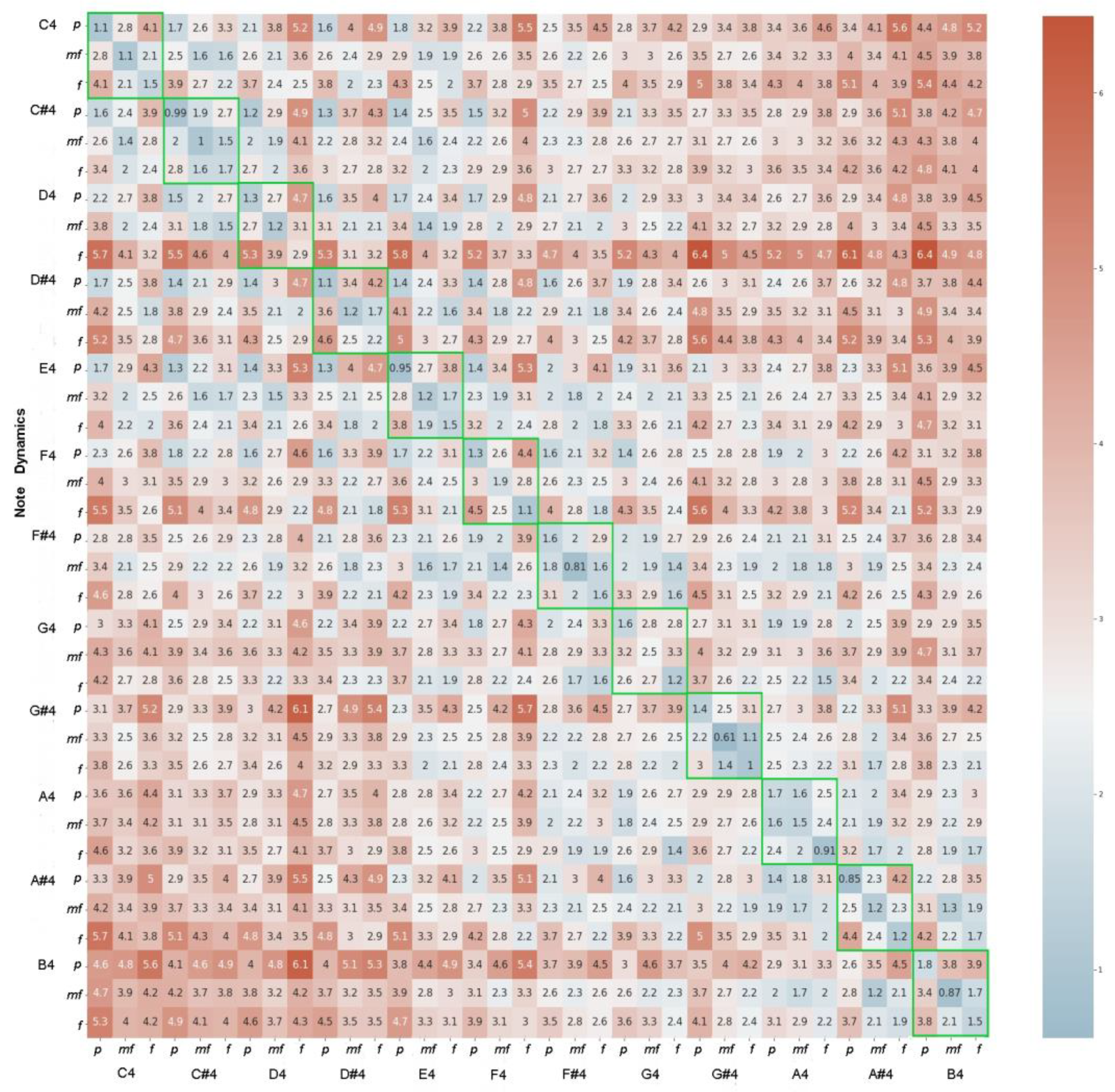
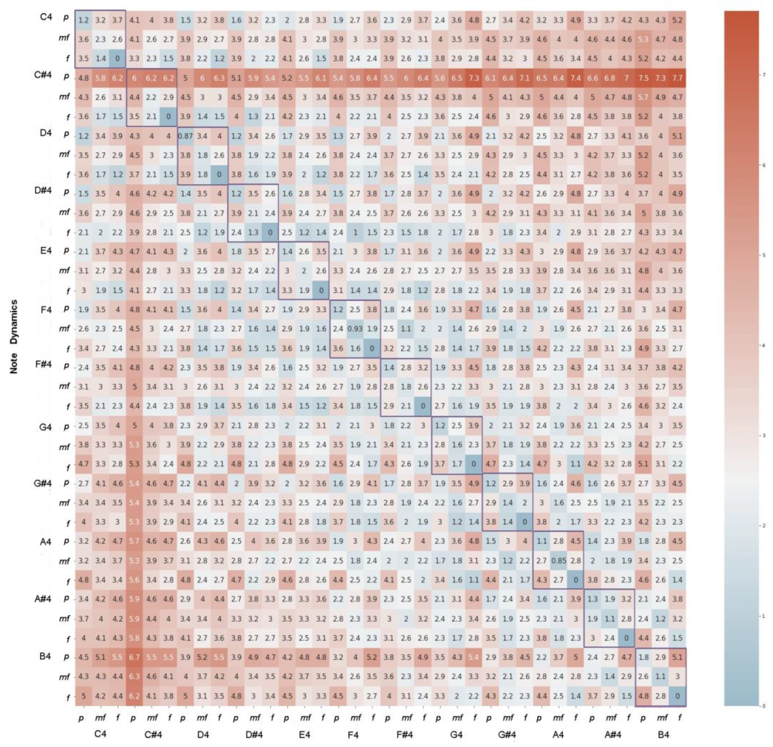
4.2. Variations Due Musical Dynamics

When variations of the dynamics are considered for the sounds of the fourth octave, we observed that the minimum distance occurs precisely for the correspondence between the sounds (diagonal elements). In Figure 4(up) Clarinet and Figure 4(down) Flute, it was observed that, in each row, the minimum distance occurs for the corresponding sound on the musical and dynamic scale. We also noted that the dynamics of mezzo-forte are always less than those of the adjacent sounds (by rows or columns) for all musical notes and in both instruments.
There does not seem to be a d/d_mean behavior for the various dynamics in the Clarinet. The dynamic of fortissimo in the Flute (Figure 4) is always close to the value of d_mean for each musical sound. This may be due to the fact that the monophonic sounds of the Flute are well-defined by the performer when the pressure of air is at its maximum within the resonant cavity and by the relative ease to play of this dynamic. So, for the sounds of the flute in fortissimo, the execution is very similar in different interpreters, and the dispersion of distance values in the registers is smaller. That is, the standard deviation of the sample is very small (d/d_mean was less than a tenth of the standard deviation).

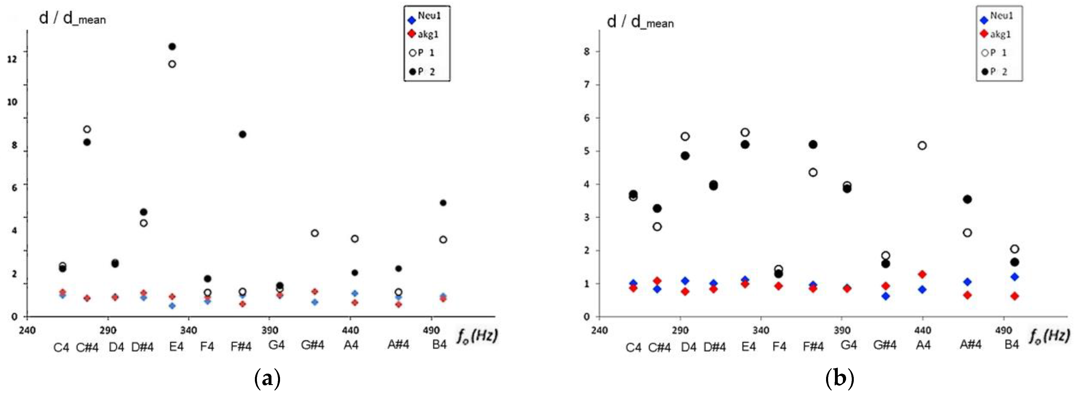
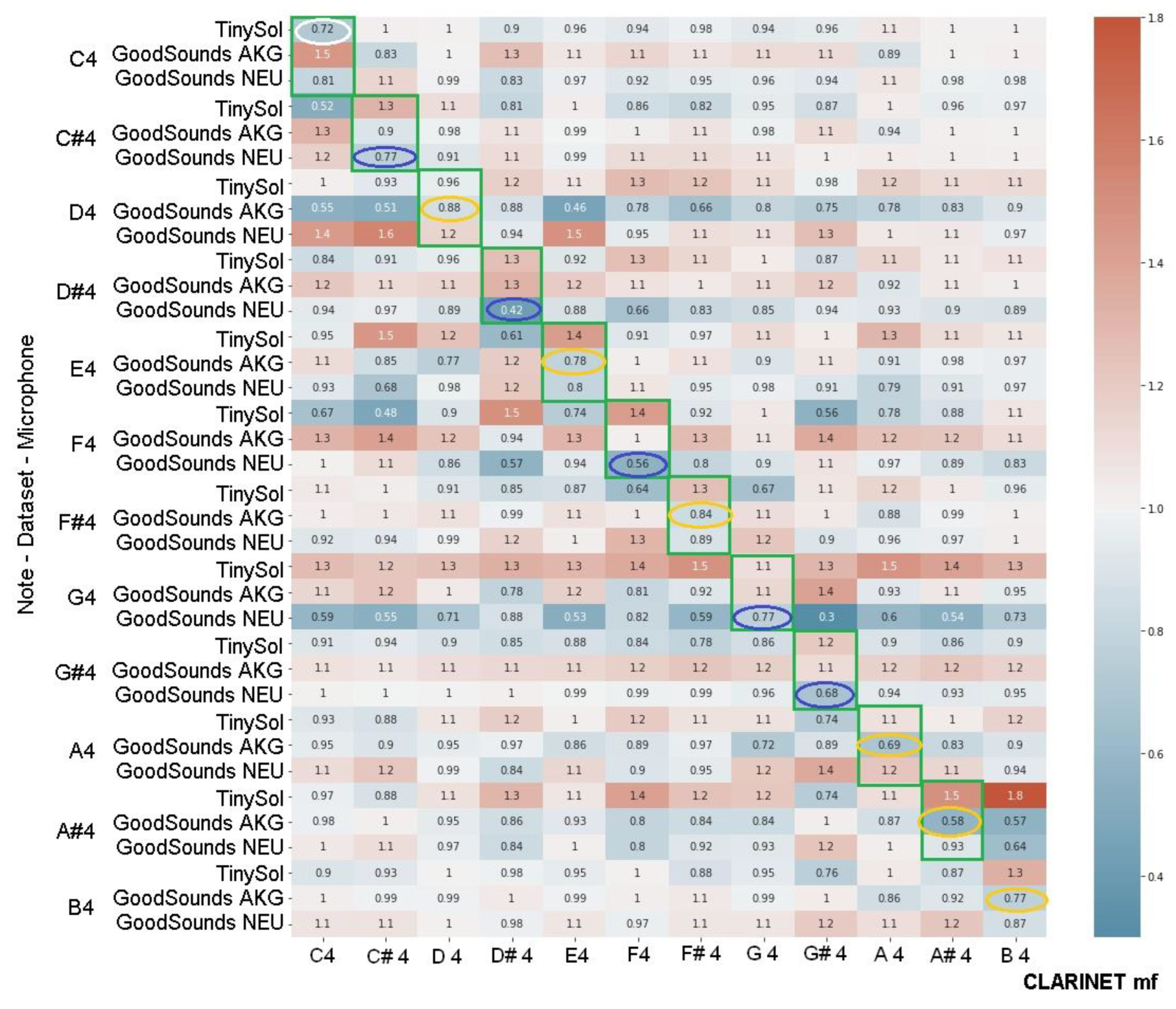
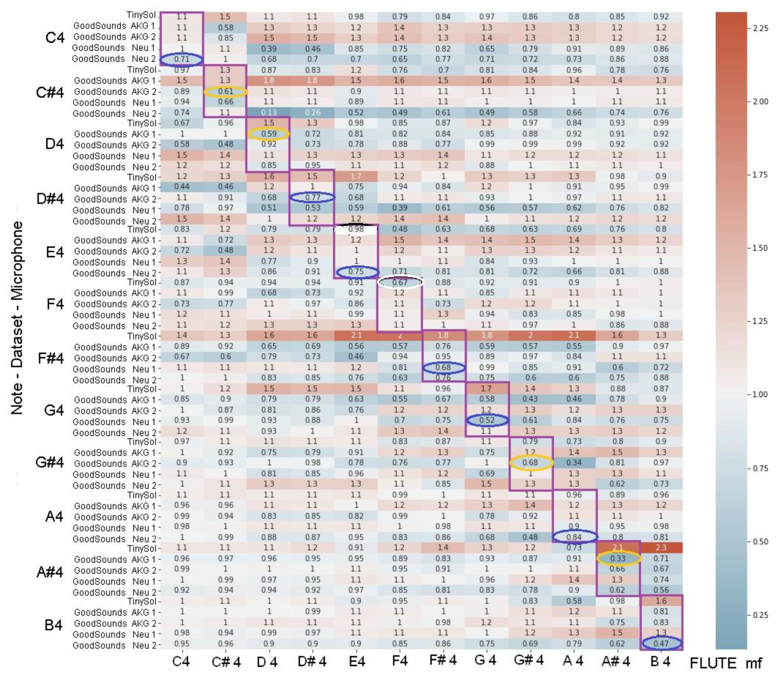
4.3. Variations Due to the Tinysol and GoodSounds Database

The classification of the timbre of musical instruments in the proposed seven-dimensional space critically depends on the standardization of the real audios taken as reference. For this reason, it is important to ensure the robustness and reliability of the reference audio records. The databases used, as already mentioned, are reliable [32,33]; the standardized distances of the records for Clarinet and Flute are shown in Figure 5 and Figure 6, respectively, and are grouped by dataset type (Tinysol, Goodsounds-Neumann, and Goodsounds-AKG). Figure 5 and Figure 6 show that the audio records are within the radius of reliability radius of the normal distribution, with the separation from the mean value less than 2.2 times the standard deviation.
The diagonal sub-blocks of the matrix indicate the correspondence with the expected values for the ratio between d/d_mean. The minimum value in each data set has been highlighted. For the Clarinet, the GoodSounds Neumann audio recordings are closer to the mean value and better discriminate the smallest distance in relation to the other distances of the other sounds (minimum value for each row, highlighted in dotted ovals). Figure 6 shows the comparison of the Transverse Flute data sets. The GoodSounds database provides two sets of Neumann-type and AKG-type records.
For some sounds, the distance closest to the mean value belongs to different recordings with no apparent systematic variation. However, the mode with which a given database provides a weighted distance (d/d_mean) closest to the mean value could be used as a quantitative evaluation criterion for various sound libraries.

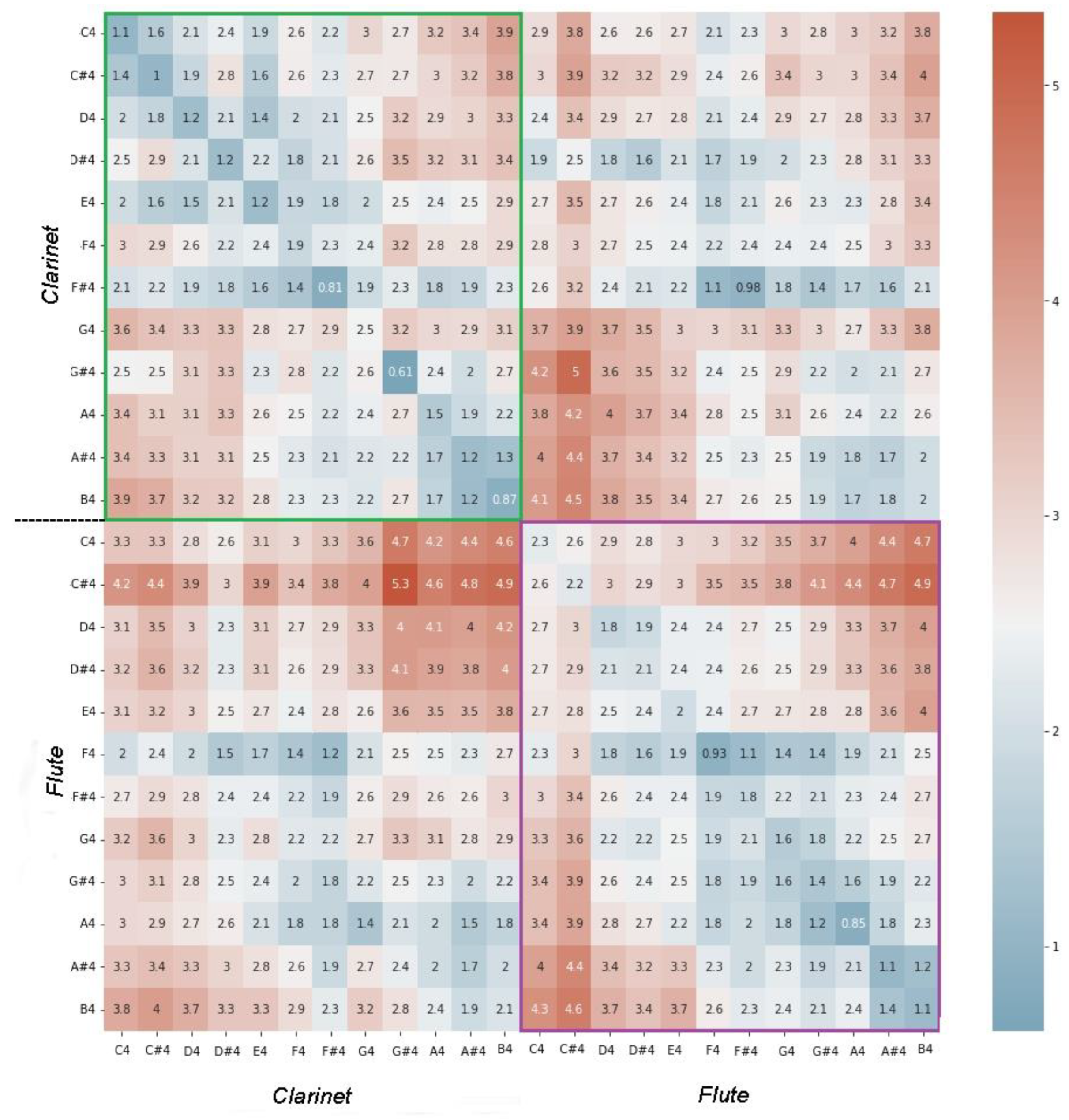
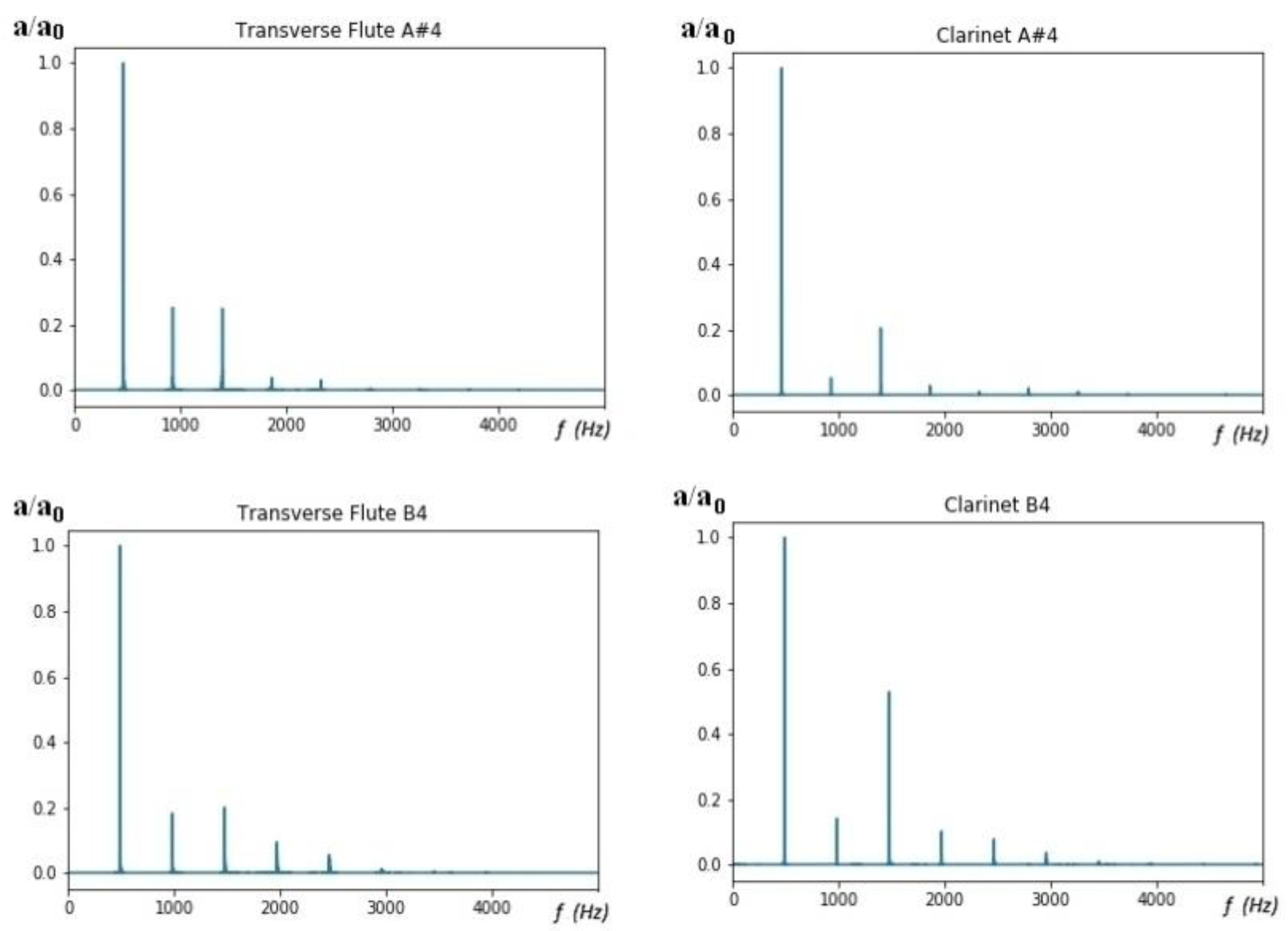
4.4. Timbral Similarity between Clarinet and Transverse Flute

For the common tessiture between Clarinet and Flute in mezzo-forte dynamics, the results of timbral distances (Figure 2) can be used to find those sounds generated by different instruments such that the separation in timbral space is statistically significant (less than 2.4 times the average of the distance), in accordance with the machine-learning algorithm presented in Figure 1. Table 1 shows the distance values between similar sounds for the fourth octave. Note that the minimum distance corresponds to the diagonal elements, as expected. However, there are sounds between different instruments that are also significant because their distance is less than 2.4 times of the average distance. This suggests that they are timbrically related, that is to say that the FFTs of these sounds should be similar in terms of the number of harmonics, envelopes, and distribution of partial frequencies. Indeed, in Figure 7 the FFTs are shown where it is possible to see their similarity.

5. Conclusions

The septuple made up of the fundamental frequency and the six timbral coefficients of each musical sound unambiguously define a collection of points and, therefore, formally (Category Theory), a timbral space can be devised to represent the sounds. In such a space, the subsets of musical sounds are groupoids and are related to each other by morphisms. This suggests that for each musical instrument, the dynamics and musical sound would be represented by a single characteristic vector (f0, A, S, H, M, AM, CM) containing significant timbral characteristics. The real audio recordings would constitute statistical variations due to randomness in the execution of the musical sound by the interpreter and to specificities of the musical instrument with which the audio was made (model and manufacturer, quality of the same, materials used, imperfections of its acoustics, etc.), or even the recording equipment. Then, the audio sets for a type of musical instrument, specific dynamics, and a specific sound, will cover a spatial region in addition to the characteristic timbral vector.
In this work, we were able to determine the timbral variations of the following audio categories:
-
Audios of different sounds and different instruments (Section 4.1).
-
Audios of the same type of sound and instrument with different relative musical dynamics (Section 4.2).
-
Audios of different databases (Section 4.3).
We find that for all the case studies, the smallest distances always occur between the elements of the diagonal. In the case of timbral variations by dynamics, we found that for most of the sounds, the dynamics of pianissimo and mezzo-forte have the smallest distances. This is related to the acoustic properties of the instrument and the difficulty of the air control for the dynamics of fortissimo by the performers. Regarding the analyzed databases, we found that the GoodSounds—Neumann database was the one with the lowest distance values. This suggests that it is a more reliable database for analysis of timbral properties of instruments.
For the study of the timbral similarities between the audio recordings, we proposed an algorithm (Figure 1) that evaluates such timbral similarities through Euclidean distances in the abstract space of 7 dimensions. This allowed us to find which FFTs are similar across different instruments (Section 4.4). For the two instruments in this study, statistically significant sounds were found because their distance is less than 2.4 times of the average distance. This suggests that these sounds (Table 1) are timbrically related, that is, that the FFTs of these sounds are similar in terms of the number of harmonics, envelope, and distribution of partial frequencies.
We plan to investigate different machine learning algorithms for future work, as well as different measures of distance.

Author Contributions

Conceptualization, Y.G. and R.C.P.; methodology, Y.G. and R.C.P.; software, Y.G. and R.C.P.; validation, Y.G. and R.C.P.; formal analysis, Y.G. and R.C.P.; investigation, Y.G. and R.C.P.; resources, Y.G. and R.C.P.; data curation, Y.G. and R.C.P.; writing—original draft preparation, Y.G.; writing—review and editing, Y.G. and R.C.P.; visualization, Y.G.; supervision, R.C.P.; project administration, Y.G. and R.C.P.; funding acquisition, Y.G. and R.C.P. All authors have read and agreed to the published version of the manuscript.

Funding

This study was financed in part by the Coordenação de Aperfeiçoamento de Pessoal deNível Superior—Brasil (CAPES)—Finance Code 001.

Institutional Review Board Statement

Not applicable.

Informed Consent Statement

Not applicable.

Data Availability Statement

The sounds used in this work are available at the following link: https://zenodo.org/record/3685367#.XnFp5i2h1IU%22, accessed on 15 May 2022.

Conflicts of Interest

The authors declare no conflict of interest.

References

  1. Jiang, W.; Liu, J.; Zhang, X.; Wang, S.; Jiang, Y. Analysis and Modeling of Timbre Perception Features in Musical Sounds. Appl. Sci. 2020, 10, 789. [Google Scholar] [CrossRef]
  2. Guven, E.; Ozbayoglu, A.M. Note and Timbre Classification by Local Features of Spectrogram. Procedia Comput. Sci. 2012, 12, 182–187. [Google Scholar] [CrossRef]
  3. Fourer, D.; Rouas, J.L.; Hanna, P.; Robine, M. Automatic timbre classification of ethnomusicological audio recordings. In Proceedings of the International Society for Music Information Retrieval Conference (ISMIR 2014), Taipei, Taiwan, 27–31 October 2013. [Google Scholar]
  4. McAdams, S. The perceptual representation of timbre. In Timbre: Acoustics, Perception, and Cognition; Springer: Cham, Switzerland, 2019; pp. 23–57. [Google Scholar]
  5. Liu, J.; Zhao, A.; Wang, S.; Li, Y.; Ren, H. Research on the Correlation Between the Timbre Attributes of Musical Sound and Visual Color. IEEE Access 2021, 9, 97855–97877. [Google Scholar]
  6. Reymore, L.; Huron, D. Using auditory imagery tasks to map the cognitive linguistic dimensions of musical instrument timbre qualia. Psychomusicol. Music. Mind Brain 2020, 30, 124–144. [Google Scholar] [CrossRef]
  7. Reymore, L. Characterizing prototypical musical instrument timbres with Timbre Trait Profiles. Musicae Sci. 2022, 26, 648–674. [Google Scholar] [CrossRef]
  8. Muller, M.; Ewert, S.; Kreuzer, S. Making chroma features more robust to timbre changes. In Proceedings of the 2009 IEEE International Conference on Acoustics, Speech and Signal Processing, Taipei, Taiwan, 19–24 April 2009; pp. 1877–1880. [Google Scholar] [CrossRef]
  9. Muller, M. Fundamentals of Music Processing; Springer: Erlangen, Germany, 2021. [Google Scholar]
  10. Muller, M.; Ewert, S. Towards Timbre-Invariant Audio Features for Harmony-Based Music. IEEE Trans. Audio Speech Lang. Process. 2010, 18, 649–662. [Google Scholar] [CrossRef]
  11. Lartillot, O.; Toiviainen, P.; Eerola, T. A Matlab Toolbox for music information retrieval. In Data Analysis, Machine Learning and Applications; Springer: Berlin/Heidelberg, Germany, 2008; pp. 261–268. [Google Scholar]
  12. Peeters, G.; Giordano, B.L.; Susini, P.; Misdariis, N.; McAdams, S. The timbre toolbox: Extracting audio descriptors from musical signals. J. Acoust. Soc. Am. 2011, 130, 2902–2916. [Google Scholar] [PubMed]
  13. Barbedo, J.G.; Tzanetakis, G. Musical instrument classification using individual partials. In IEEE Transactions on Audio, Speech, and Language Processing; IEEE: New York, NY, USA, 2010; Volume 19, pp. 111–122. [Google Scholar]
  14. Joshi, S.; Chitre, A. Identification of Indian musical instruments by feature analysis with different classifiers. In Proceedings of the Sixth International Conference on Computer and Communication Technology 2015, Allahabad, India, 25–27 September 2015; pp. 110–114. [Google Scholar] [CrossRef]
  15. Ezzaidi, H.; Bahoura, M.; Hall, G.E. Towards a characterization of musical timbre based on chroma contours. In Proceedings of the International Conference on Advanced Machine Learning Technologies and Applications, Cairo, Egypt, 8–10 December 2012; pp. 162–171. [Google Scholar]
  16. Böck, S.; Korzeniowski, F.; Schlüter, J.; Krebs, F.; Widmer, G. Madmom: A new python audio and music signal processing library. In Proceedings of the 24th ACM International Conference on Multimedia, Santa Barbara, CA, USA, 23–27 October 2016; pp. 1174–1178. [Google Scholar]
  17. McFee, B.; Raffel, C.; Liang, D.; Ellis, D.P.; McVicar, M.; Battenberg, E.; Nieto, O. Librosa: Audio and music signal analysis in python. In Proceedings of the 14th Python in Science Conference, Austin, TX, USA, 6–12 July 2015; Volume 8, pp. 18–25. [Google Scholar]
  18. Krimphoff, J.; McAdams, S.; Winsberg, S. Characterization of the timbre of complex sounds. II Acoustical analysis and psychophysical quantification. J. Phys. 1994, 4, 625–628. [Google Scholar]
  19. Johnston, J. Transform coding of audio signals using perceptual noise criteria. IEEE J. Sel. Areas Commun. 1988, 6, 314–323. [Google Scholar]
  20. Gaikwad, S.; Chitre, A.V.; Dandawate, Y.H. Classification of Indian Classical Instruments using Spectral and Principal Component Analysis based Cepstrum Features. In Proceedings of the IEEE International Conference on Electronic Systems, Signal Processing and Computing Technologies (ICESC), Nagpur, India, 9–11 January 2014. [Google Scholar]
  21. Joder, C.; Slim Essid, S. Temporal Integration for Audio Classification with Application to Musical Classification. In IEEE Transaction on Speech and Audio Processing; IEEE: New York, NY, USA, 2009; Volume 17, pp. 174–186. [Google Scholar]
  22. Pollard, H.F.; Jansson, E.V. A tristimulus method for the specification of musical timbre. Acta Acust. United Acust. 1982, 51, 162–171. [Google Scholar]
  23. Burred, J.J.; Röbel, A.; Sikora, T. Dynamic spectral envelope modeling for timbre analysis of musical instrument sounds. IEEE Trans. Audio Speech Lang. Process. 2010, 18, 663–674. [Google Scholar]
  24. Gonzalez, Y.; Prati, R.C. Acoustic Descriptors for Characterization of Musical Timbre Using the Fast Fourier Transform. Electronics 2022, 11, 1405. [Google Scholar] [CrossRef]
  25. Gonzalez, Y.; Prati, R.C. Applications of FFT for timbral characterization in woodwind instruments. In Proceedings of the Brazilian Symposia On Computer Music (SBCM), Recipe, PE, Brazil, 24–27 October 2021. [Google Scholar] [CrossRef]
  26. Gonzalez, Y.; Prati, R.C. Acoustic Analysis of Musical Timbre of Wooden Aerophones. Rom. J. Acoust. Vib. 2022; in press. [Google Scholar]
  27. Cella, C.E.; Ghisi, D.; Lostanlen, V.; Lévy, F.; Fineberg, J.; Maresz, Y. OrchideaSOL: A dataset of extended instrumental techniques for computer-aided orchestration. arXiv 2020, arXiv:2007.00763. [Google Scholar]
  28. Awodey, S. Category Theory; Oxford University Press: Oxford, UK, 2010. [Google Scholar]
  29. Mannone, M.; Arias-Valero, J.S. Some Mathematical and Computational Relations Between Timbre and Color. In Mathematics and Computation in Music. MCM 2022. Lecture Notes in Computer Science; Montiel, M., Agustín-Aquino, O.A., Gómez, F., Kastine, J., Lluis-Puebla, E., Milam, B., Eds.; Springer: Cham, Switzerland, 2022; Volume 13267, pp. 127–139. [Google Scholar]
  30. Grey, J.M. Multidimensional perceptual scaling of musical timbres. J. Acoust. Soc. Am. 1977, 61, 1270–1277. [Google Scholar] [PubMed] [Green Version]
  31. McAdams, S. Perception et Cognition de la Musique. 2015. Available online: https://www.erudit.org/en/journals/sqrm/2016-v17-n2-sqrm03970/1052743ar/ (accessed on 10 November 2022).
  32. Carmine, E.; Ghisi, D.; Lostanlen, V.; Lévy, F.; Fineberg, J.; Maresz, Y. TinySOL: An Audio Dataset of Isolated Musical Notes. Zenodo 2020. Available online: https://zenodo.org/record/3632193#.Y-QrSnbMLIU (accessed on 15 May 2022).
  33. Romaní Picas, O.; Parra-Rodriguez, H.; Dabiri, D.; Tokuda, H.; Hariya, W.; Oishi, K.; Serra, X. A real-time system for measuring sound goodness in instrumental sounds. In Proceedings of the 138th Audio Engineering Society Convention, AES 2015, Warsaw, Poland, 7–10 May 2015; Audio Engineering Society: New York, NY, USA, 2015; pp. 1106–1111. [Google Scholar]
Figure 1. Flowchart diagram of the algorithm to calculate distances and relations of timbral similarity.
Eng 04 00033 g001
Figure 2. Patterned distance between musical sounds for Clarinet and Flute in mezzo-forte for the 4 ta octave, reference sounds in the data set.
Eng 04 00033 g002
Figure 3. Patterned distance between musical sounds in mezzo—forte for the 4 ta octave, reference sounds in the dataset: (a) Clarinet (b) Flute.
Eng 04 00033 g003
Figure 4. Patterned distance between musical sounds for clarinet (up) and Transverse Flute (down) in several dynamics (p, mf, f) for the 4 ta octave, reference sounds in the dataset.
Eng 04 00033 g004aEng 04 00033 g004b
Figure 5. Patterned distance between musical sounds for Clarinet to reference sounds, according to several data sets. The circles of colors represent the shortest distance between the three dynamics.
Eng 04 00033 g005
Figure 6. Patterned distance between musical sounds for Flute to reference sounds, according to several data sets. The circles of colors represent the shortest distance between the sound libraries.
Eng 04 00033 g006
Figure 7. Comparison of the normalized FFTs of the sounds A#4 and B4 (rows) for Flute and Clarinet (columns). The intensities are normalized with respect to the amplitude (a0) of the fundamental frequency.
Eng 04 00033 g007
Table 1. Average distance in the timbral space of the sounds A#4 and B4 for Flute and Clarinet.
ClBb A#4ClBb B4Fl A#4Fl B4
ClBb A#41.1981.3141.6671.985
ClBb B41.1840.8671.8072.015
Fl A#41.6652.0261.0911.247
Fl B41.9362.1411.3621.127
Disclaimer/Publisher’s Note: The statements, opinions and data contained in all publications are solely those of the individual author(s) and contributor(s) and not of MDPI and/or the editor(s). MDPI and/or the editor(s) disclaim responsibility for any injury to people or property resulting from any ideas, methods, instructions or products referred to in the content.

