Presentation of a Rainfall–Runoff Retention Model (3RM) Based on Antecedent Effective Retention for Estimating Runoff in Seven Basins in Iran

Abstract

This study aims to correct and assess the SCS-CN model. In this research, the 3RM model (written by Shamohammadi) has been modified in such a way that the maximum primary retention (I), maximum secondary retention (F_max), and basin potential retention (S_max) can be calculated using precipitation (P_a). The purpose of this study is to evaluate the total retention model ($S_t=f(F_{max},S_{max},p_a)$) and the runoff model ($Q=f(S_t,p_a)$) using the mountain basins of Iran, including Emameh, Kasilian, Navrood, Darjazin, Kardeh, Khanmirza, and Mashin. The results showed that the primary retention, maximum secondary retention, and retention capacity are, respectively, 2.3, 30.4, and 32.7 mm in Imamah, 2.5, 48.6, and 51.1 mm in Kasilian, 2.4, 26.7, and 29.1 mm in Navrood, 3.2, 21.5, and 24.7 mm in Darjazin, 1.7, 15.0, and 16.7 mm in Kardeh, 2.5, 33.2, and 38.1 mm in Khanmirza, and 4.9, 44.5, and 50.6 mm in Mashine. Additionally, the λ (ratio of primary retention to potential retention) values for all basins are less than 0.2 (suggested by SCS) and vary between 0.05 in Kasilian and 0.1 in the Darjazin, Kardeh, and Mashine basins. The results of fitting the model to the rainfall-runoff data showed that the evaluation indices, including the coefficient of determination (R²), Nash–Sutcliffe (NS), and root mean square error (RMSE), for predicting the runoff in the basins varied between 0.78 to 0.96, 0.78 to 0.961, and 0.86 to 2.28, respectively. According to the obtained results, it can be concluded that the model has an acceptable ability to predict runoff for all the studied basins.

1. Introduction

With the progress of computer science, it is necessary to develop hydrological models along with the development of information technology, and instead of using descriptive methods and curve numbers, use data-driven models to predict floods and runoff [1]. One of the widely used methods in runoff estimation is the SCS-CN experimental method [2]. In this method, the classification of soil moisture conditions in each area is carried out only according to five-day antecedent rainfall and the growing and dormant season; this classification has a significant effect on determining the curve numbers and, finally, the runoff [3,4,5].

A lot of research has also tried to modify and optimize the SCS-CN method, especially in case of antecedent moisture conditions [6,7,8,9,10,11] indicated that, in the SCS-CN method, the use of a revised soil-moisture index instead of the use of antecedent moisture had better results. Verma et al. [12], developed a soil moisture accounting (SMA)-based SCS-CN method to avoid sudden jumps in estimated runoff. Ogarekpe et al. [13], used modified SCS models for predicting runoff in the Oraimiriukwa River Basin. They showed that the ratio of initial interception to maximum potential retention is not constant and is a function of precipitation.

Singh et al. [14], showed that one of the most important limitations of the SCS-CN method is that slope is not considered. In the modified SCS-CN method, the slope is considered to enhance the accuracy of the modeled results.

Many researchers also considered the SCS-CN model to be ineffective and showed that the SCS-CN method does not have the necessary efficiency for Karst landforms and forest areas [15,16,17]. Vaezi and Abbasi [18], investigated the efficiency of the SCS-CN curve number method for estimating the runoff in the Tehmchai Basin (in the northwest of Iran) and showed that the λ was <0.2. As a result, they suggested that the coefficient λ = 0.2 is not correct and the value of λ needs to be calibrated. These results were also repeated for the Kardeh Basin by Ebrahimian et al. [19].

Shamohammadi and Zomorodian [20], compared the performance of the SCS and Bennett Soil Moisture Accounting (SMA-B) models in estimating the flood in the Roodzard Basin in Iran. The results of this research indicated the inefficiency of the SCS model when compared to the SMA-B model. The results of the studies of Sadeghi et al. [21] also showed that the SCS-CN method is weak in estimating the runoff of the Emameh, Kasilian, Darjazin, and Khanmirza basins (in Iran). Similar research was also conducted by Asadi et al. [22], Arand and Torabi [23], Shammohammadi [24], and Orak and Farhadi [25] for the Mashin and Navrood basins, and it shows the weakness of the SCS-CN method for estimating runoff.

Shamohammadi [26], showed that the mathematical model of SCS-CN has a theoretical weakness and is basically unable to describe the conceptual model of SCS-CN. He stated that each basin has only one potential retention (S_max or S_p) and one secondary potential retention (F_max). Both of them are obtained through their variable parameters (F and S_t, respectively).

Shamohammadi wrote his mathematical model based on the function variable F (secondary retention) and used the constant coefficient K_sh [26]. The most important weakness of the Shamohammadi model is that it was necessary to use the linear regression between rainfall-runoff data to calculate the initial retention (I). In the current research and in the Shamohammadi model (modified 3RM), instead of F, the total retention function (S_t) is used, and instead of the K_sh coefficient, the secondary maximum retention (F_max) is used. 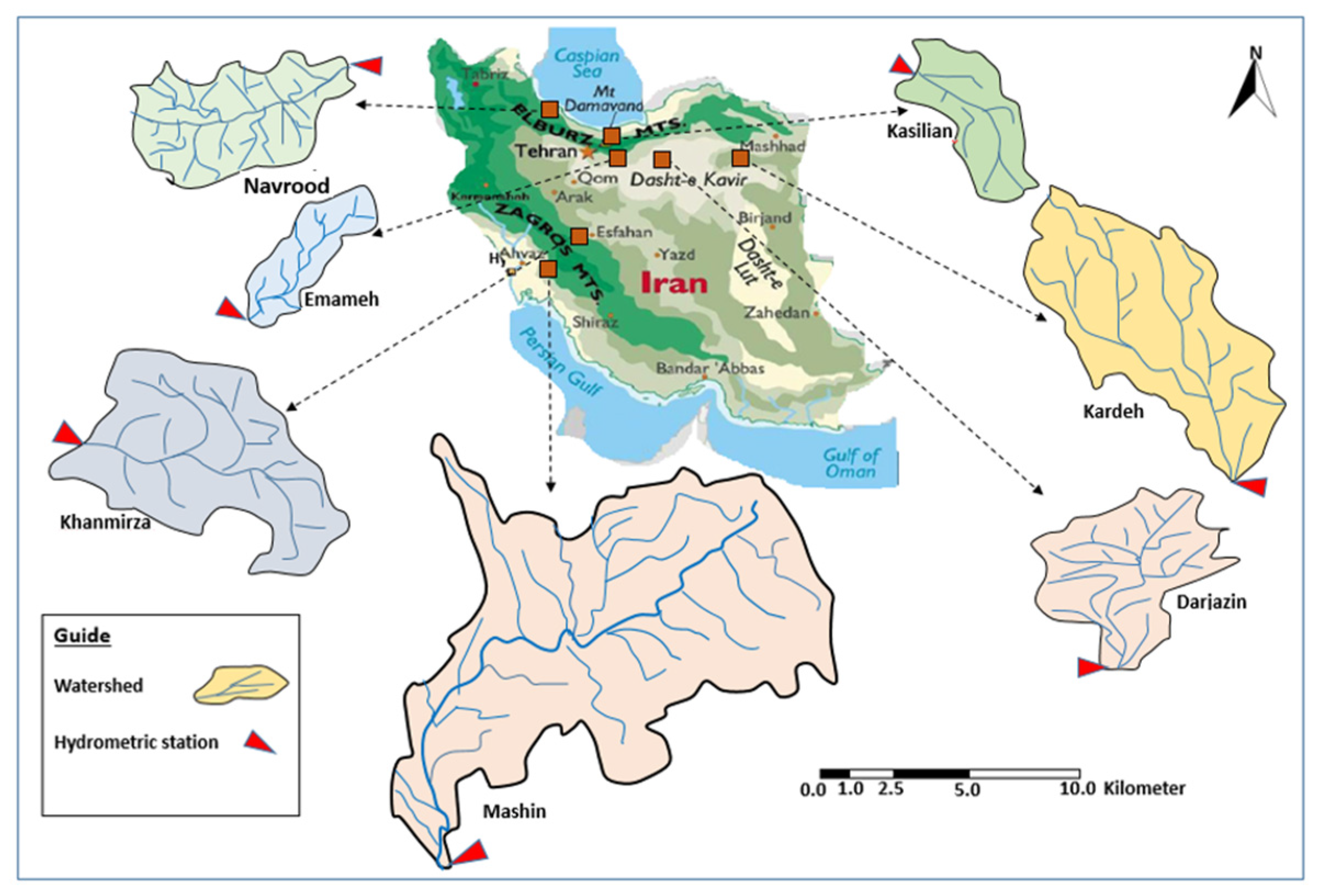As a result, while reducing the error in the calculation of initial retention (I), the values of I, F_max, and S_max are directly extracted from the model (innovation of the present research), and the model also becomes simpler. In order to evaluate the new model, data from different areas of Iran (seven basins with different areas, different climates, and different landforms in the important mountain ranges of Iran) were used.

1.1. An Introduction to the Model

1.1.1. Definitions

I: Initial retention: this includes all the factors that prevent the creation of runoff (water runoff, impoundments, infiltration, evaporation, etc.). This parameter is constant for a basin and is equal to the sum of the initial retention (I_a) and the antecedent effective retention (I_ER) (I = I_a + I_ER). It is obvious that the value of I varies from each type of rainfall to another, but it is generally a constant value for a basin.

F: Secondary retention (in this study, secondary retention is used instead of actual retention): this includes all the factors that prevent runoff. The only difference between F and I is that F occurs at the beginning of the rainfall event, while I is related to retention before runoff. The value of F is variable in basins.

S_t: Total retention: this is equal to F + I, so S_t is also variable.

S_max: The maximum retention or potential retention (S_p) is the maximum retention after which rainfall is completely converted into runoff. Theoretically, when the rainfall tends to infinity, all the impoundments are filled, the soil is saturated, and even the air humidity reaches the saturation limit. As a result, after retention is equal to S_max, all rainfall converts to runoff. In this case, the slope of the rainfall-runoff curve will be equal to 1. It is obvious that the potential retention is an ideal and hypothetical condition for the dry state of the soil and can only be calculated through the model. In the SCS-CN method, the potential retention is estimated using the curve number, which, in the correct case, is a real number (it is part of the storage potential) and cannot be storage potential. This also applies to F_max.

F_max: It is defined as S_max and is linearly constant. Its relationship with S_max is as $F_{max}=S_{max}-I$.

I_ER: Antecedent effective retention: this is a part of retention due to antecedent rainfall (P_A), which is effective in the rainfall-runoff system and is calculated as per Equation (1) [27]:

$$I_{ER}=P_A-\left[Q_A+{\left({\sum }_{n1}^{n_t}{ET}_0\right)}_A\right]$$

(1)

where P_A, Q_A, and (ET₀)_A are the antecedent rainfall depth, antecedent runoff depth, and the daily antecedent potential evapotranspiration, respectively, and n₁ and n_t are the days of the beginning of the antecedent and the target, respectively.

Additionally, it can always be written as per Equation (2):

$$Q=P_a-S_t$$

(2)

$${P_a=P+I}_{ER}$$

where Q and P_a are the runoff depth (mm) and the modified target rainfall depth (mm), respectively.

1.1.2. Assumptions of the Shamohammadi Model

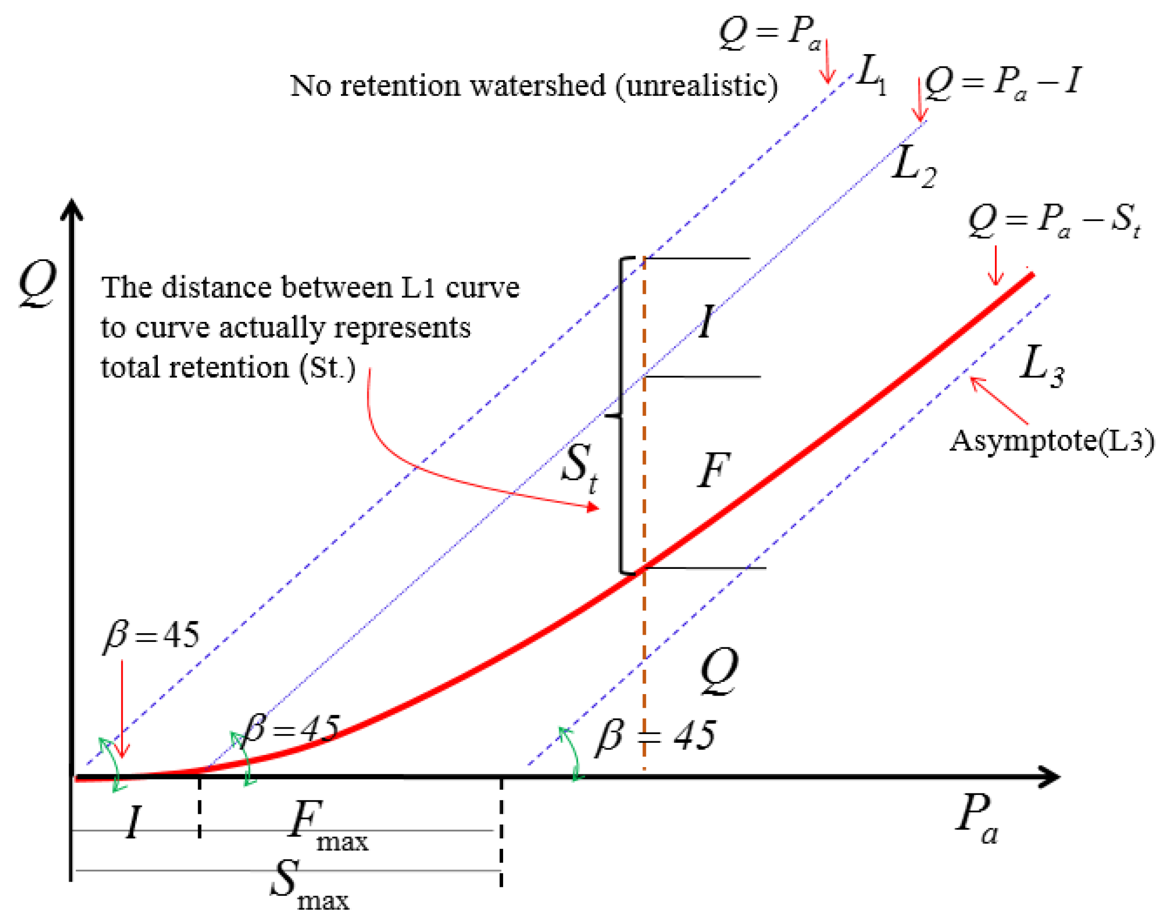
Equations (3) and (4) have been presented for the mathematical description of the conceptual curve in Figure 1.

$$\frac{dQ}{d{p}_a}=\frac{S_t}{S_{max}}$$

(3)

$$\frac{d{S}_t}{d{p}_a}=\frac{K_{sh}}{K_{sh}+p_a}$$

(4)

In Equation (4), the K_sh is the Shamohammadi constant. Additionally, $\frac{dQ}{d{p}_a}$ and $\frac{d{S}_t}{d{p}_a}$ are the differential of runoff (compared to corrected rainfall) and the differential of total retention to rainfall, respectively. The other parameters are already defined.

On the other hand, based on the law of the survival of the fittest, it follows that

$$P_a=S_t+Q$$

(5)

Equation (5) is a general equation. Obviously, when the runoff is equal to 0, P_a = S_t = I, and when the total retention is completed and when rainfall is converted to runoff, then P_a = Q.

Using differentiation on both sides of Equation (5) with respect to rainfall, we obtain the following:

$$\frac{d{P}_a}{d{P}_a}=\frac{d{S}_t}{d{P}_a}+\frac{dQ}{d{P}_a}$$

(6)

Finally, Equation (6) can be written as Equation (7):

$$1=\frac{d{S}_t}{d{P}_a}+\frac{dQ}{d{P}_a}$$

(7)

Considering Equations (3), (4), and (7), we can write the following as Equation (8):

$$1=\frac{k_{sh}}{k_{sh}+P_a}+\frac{S_t}{S_{max}}$$

(8)

and then (Equation (9)):

$${S_t=S}_{max}\frac{P_a}{k_{sh}+P_a}$$

(9)

According to Equation (9), when the rainfall tends to I (P_a→I), the value of K_sh will be equal to F_max because when the rainfall is equal to I, the value of S_t will also be equal to I (F = 0) as a result:

$$\{\begin{array}{c}I=S_{\mathit{max}}\frac{l}{k_{\mathit{sh}}+I}\to S_{\mathit{max}}=k_{\mathit{sh}}+I\hfill \\ k_{\mathit{sh}}=S_{\mathit{max}}-I\hfill \end{array}$$

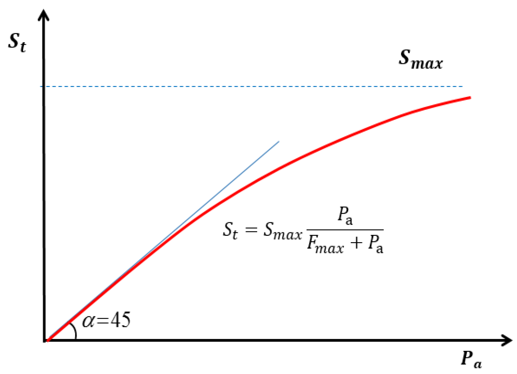
However, based on the conceptual model in Figure 1 and the definition of F_max, the value of k_sh is equal to F_max. Therefore, Equation (9) is modified as per Equation (10). Figure 2 shows the schematic of the maintenance of Equation (10).

$${S_t=S}_{max}\frac{P_a}{F_{max}+P_a}$$

(10)

According to the relationship between runoff and total retention (Equation (2)), the amount of runoff depth is equal to what follows in Equation (11):

$${Q=P_a-S}_{max}\frac{P_a}{F_{max}+P_a}$$

(11)

The first advantage of model (11) compared to Shamohammadi’s model [27] is that, in the current model, the value of I is simply obtained (S_max − F_max). In this case, in addition to the error caused by linear regression being removed, the value of F_max is also easily calculated by the model. As a result, model (11) is introduced as the modified model of Shamohammadi, and by applying boundary conditions, the correctness of the model (theoretically) is also proven because $\underset{P_a\to 0}{\mathit{lim}}\left(Q\right)=0$, $\underset{P_a\to \mathrm{\infty }}{\lim (}Q)=\mathrm{\infty }$ and $\underset{P_a\to I}{\lim (}\mathrm{Q})=0$.

Therefore, model (11) is also correct in limiting the conditions (based on the definitions and assumptions of the model) and is in harmony with the conceptual model (Figure 1) and the SCS-CN conceptual model [26].

This is despite the fact that, in the SCS-CN model, when the rainfall tends to 0 (P_a→0), the runoff depth (Q) does not become zero but becomes equal to 0.05S (Equation (12)). However, in reality, when the rainfall is zero, there is no runoff. As a result, it can be said that the SCS-CN model has a theoretical weakness in its hypotheses [26]. Even if it is claimed that the SCS-CN method is an experimental method, the influence of the theoretical weakness of the model on the experimental parameters cannot be ignored. Perhaps for this reason, the SCS-CN mathematical model is not defined for rainfall less than I (0.2S) following Equation (12):

$$Q=\frac{{(P-0.2S)}^2}{P+0.8S}P\ge 0.2S$$

(12)

Equations (10) and (11) are the basis equations for runoff estimation in this study. As mentioned before, the conceptual model of Figure 1 is the SCS-CN conceptual model. Only its hydrological parameters have been revised and redefined. Therefore, although Shamohammadi’s mathematical model is completely consistent with the SCS-CN conceptual model, it is completely different from the SCS-CN mathematical model (12) (both in terms of the relationships between the parameters and in terms of the method used for solving the problem). As a result, some of the SCS-CN limitations are also present in the current model, some of which are mentioned below:

• The basin area should be so small that the whole basin is covered by rainfall (uniformly and at a constant intensity);
• The intensity of different rainfalls should be equal to each other so that the runoff is only caused by the depth of the rainfall. Increasing the intensity of the rainfall causes runoff before the completion of primary retention; on the other hand, it causes an increase in mud in the runoff; thus, the amount of runoff at the hydrometric station is measured more than the actual runoff;
• This model (SCS-CN) was developed for natural basins. In a basin (especially large basins), if there are man-made structures such as earthen dams, pools, large dry streams, or any unnatural structures, the data are not based on the theory of the conceptual model theory and, as a result, the models will not be able to correctly analyze the situation;
• Accurate results can be expected from the model (11) when the rainfall-runoff curve follows the conceptual curve of Figure 1. Otherwise, the rainfall-runoff data must be checked carefully, and the incorrect data (for example, when the rainfall did not cover the entire basin) must be corrected or removed.

Of course, the limitations of the current model are much less than the SCS-CN model because it is based on historical data and operates as a black box model. In other words, in this model, in addition to the man-made structures, the changes in the parameters from one rainfall event to another also cause errors in the results.

2. Material and Methods

2.1. Studied Areas

In this study, the basins of Emameh, Kasilian, Navrood, Darjazin, Kardeh, Khanmirza, and Mashin, which were equipped with rain gauges and hydrometer stations, were studied. The selection of these basins was based on the quality of rainfall and runoff data, the distribution of rainfall, climate diversity, vegetation diversity, area size, and geological conditions. Figure 3 shows the location of the studied basin in Iran. The general characteristics of the basins are also shown in

Table 1. General characteristics of Emameh, Kasilian, Navrood, Darjazin, Kardeh, Khanmirza, and Mashin basins in Iran.

Basin
Basin Features	Mashin	Khanmirza	Kardeh	Darjazin	Navrood	Kasilian	Emameh
Longitude	49°39′	50°55′	41°35′	53°12′	48°34′	53°8′	51°35′
	50°10′	51°18′	47°39′	53°29′	48°54′	53°15′	57°35′
Latitude	31°21′	31°32′	31°37′	35°59′	37°36′	35°58′	51°32′
	31°41′	31°37′	35°51′	36°59′	37°47′	36°07′	51°38′
Area (km2)	882	391	547	331	260	67	37
Mean Elevation (m)	2101	231	2087	2152	1573	1620	2620
Slope (%)	7.3	45.8	7.67	14.6	7.67	15.80	7.5
Mean annual precipitation (mm)	757	814	1338	385	376	570.6	480
Mean annual temperature (°C)	9.3	9.2	11.5	9.8	11.5	12.1	25/7
Climate (De Martonne)	Arid	Arid and cold	Arid and semi-arid	Semi-arid	Semi-humid	Very humid	Humid

.

All the meteorological and rainfall-runoff data were obtained from the Iranian Meteorological Organization and Iranian Water Resources Company, covering the period of 1985–2021. Due to the fact that an earthen dam was built in the Mashin area in 2001 and caused a change in the flood conditions of the basin, the data of the Mashin station from 1978 to 2001 were studied. In this research, Landsat 8 satellite images from 2013 were used to study land use and basin features.

In the present study, to simplify model (1), all the days between the beginning of the antecedent rainfall and the beginning of the target rainfall were added together, and 315 days were obtained. Additionally, the total potential evapotranspiration for all these days (315 days) was 159 mm. As a result, the average of potential evapotranspiration was approximately equal to 0.5 mm/day (${ET}_0=\frac{{\left(\sum _{n1}^{n_t}{ET}_0\right)}_A}{315}\approx 0.5\mathrm{m}\mathrm{m}/\mathrm{d}\mathrm{a}\mathrm{y}$). Then, the average of potential evapotranspiration was used. On the other hand, no runoff has occurred in any of the antecedent rainfalls. As a result, based on [26], in this research, Equation (1) was used to simplify Equation (13).

$$I_{ER}\left(\mathrm{m}\mathrm{m}\right)=P_A\left(\mathrm{m}\mathrm{m}\right)-0.5\mathrm{D}\left(\mathrm{d}\mathrm{a}\mathrm{y}\right)$$

(13)

where D is the number of days of evapotranspiration (n_t − n₁).

The maximum number of days for calculating evapotranspiration before the target precipitation was considered to be 5 days [2,28].

2.2. Model Evaluation

The following steps were taken to run the model:

• The floods for which the associated rainfall covered the entire basin were selected. This depended on the number of rain gauge stations in the basin (between five rain gauges in the Emameh basin and 15 in the Mashin basin);
• The rainfall data for which the amount of flood was as high as the target rainfall (P, Q) were selected. Then, based on the start date of the target rainfall (P), the rainfalls that occurred (at most) 5 days before (P_A) were also determined. Because the antecedent rains did not have runoff, only the antecedent rain was recorded;
• In the case of rainfall-runoff data that did not match the conceptual curve (mostly related to large basins, especially in the Mashin Basin), the data were corrected;
• Model (11) was calibrated using half of the data. Then, using the calibrated model, the rest of the data were examined, and finally, the model was evaluated using the evaluation indices;
• Three evaluation criteria, including the coefficient of determination (R²), root mean square error (RMSE), normalized root mean square error, and the Nash–Sutcliffe coefficient (NS), were used (Equations (14)–(16)).

$$R^2={\left(\frac{{\sum }_{i=1}^N\left(Q_{obs}-\overline{Q_{obs}}\right)\left(Q_{sim}-\overline{Q_{sim}}\right)}{\sqrt{{\sum }_{i=1}^N{\left(Q_{obs}-\overline{Q_{obs}}\right)}_i^2{\left(Q_{sim}-\overline{Q_{sim}}\right)}_i^2}}\right)}^2$$

(14)

$$RMSE=\sqrt{\frac{1}{N}({\sum }_{i=1}^N{(Q_{obs}-Q_{sim})}_i^2}$$

(15)

$$NSE=1-\frac{{\sum }_{i=1}^N{\left(Q_{obs}-Q_{sim}\right)}_i^2}{{\sum }_{i=1}^N{\left(Q_{obs}-\overline{Q_{obs}}\right)}_i^2}$$

(16)

where Q_obs is the amount of observed runoff, Q_sim is the amount of simulated runoff (model), and N is the amount of data.

3. Results and Discussion

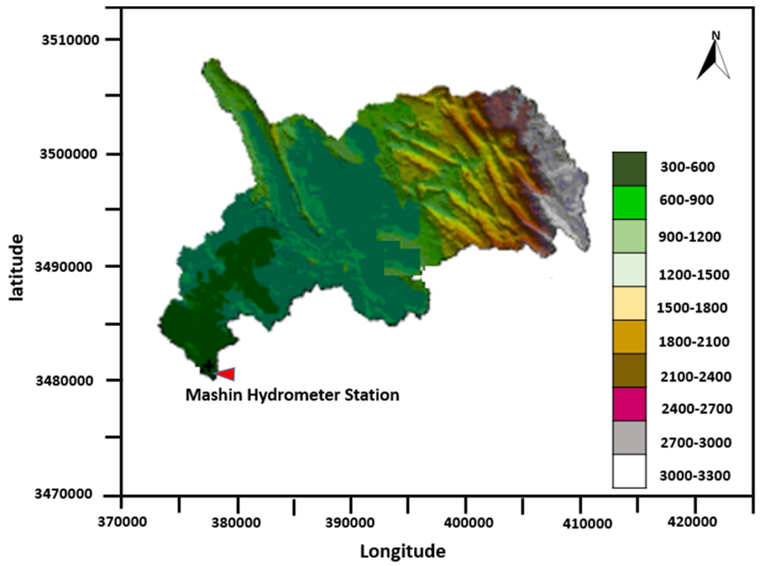
The analysis of the rainfall-runoff data of the Emameh (35 data pairs), Kasilian (73 data pairs), Navrood (24 data pairs), Darjazin (66 data pairs), Kardeh (68 data pairs), Khanmirza (28 data pairs), and Mashin (data pair 54) basins showed that 34% of all data had antecedent rainfall. The antecedent rainfall values varied between 8.7 and 1.2 mm. Maximum and minimum values were observed in the Kasilian Basin (30 October 1999) and Khanmirza Basin (25 October 2005), respectively. Additionally, the highest and lowest I_ER values occurred in the Kasilian (8.4 mm) and Darjazin (0.5 mm) basins, respectively. The ET₀ value ranged from 0.23 mm/day in the Navrood Basin (22 March 2001) to 0.65 mm/day in the Mashin Basin (28 September 1995).

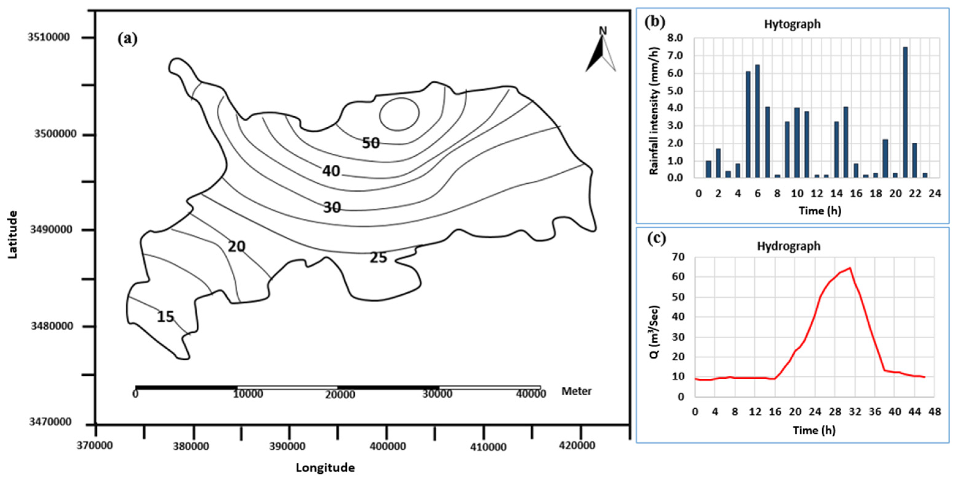
The most important challenge of this research was to select precipitations that could meet the conditions of the model. This issue is more common in large basins. One of the most challenging basins was the Mashin Basin. Figure 4 shows the isohyetal map, hyetograph, and flood hydrograph for the Mashin Basin for 1–2 April 1996. As can be seen, the depth of precipitation increases from the outlet of the basin to the north and east (Figure 4a). Additionally, the rainfall intensity (Figure 4b) has severe fluctuations during the rainfall period (23 h): two peaks of precipitation at 4 to 8 h and 20 to 23 h can be observed. Therefore, both the non-uniform intensity and depth of precipitation over 23 h are the causes of error in the model. However, due to the fact that the rainfall covers the whole basin, this error did not have much effect on the performance of the model.

One of the factors that caused the flood lag time to decrease was antecedent rainfall. The average rainfall was 71.3 mm based on the isohyetal map. On the other hand, the antecedent rainfall with a depth of 7 mm happened 5 days before. The sum of potential evapotranspiration was calculated to be 2.5 mm (0.5D = 0.5 × 5 = 2.5 mm) and the I_ER = 4.5 mm. As a result, the total amount of corrected precipitation was equal to 75.8 mm. For this reason, the runoff coefficient in this event was equal to 0.57. It is noteworthy to mention that the Mashin Basin has a Karst landform [23,25].

On the other hand, due to the low slope of the basin (7.3%) and the large area (881 km²), the obtained runoff coefficient is very large. The most important reason for this issue is probably (1) the effect of the antecedent rainfall and (2) the high-intensity rainfall. This rainfall happened in March. It was expected that the melting of snow would be involved in the volume of runoff, but the investigations showed that the height of the snow border in April in the Mashin Basin was above 2700 m [24] as a result, the effect of snow melting on the volume of the flood was very low (see Figure 5). These results are consistent with [23,25,29].

Table 2. Calibration and evaluation of the Shamohammadi model for the Emameh Basin.

IER	Calibration				Evaluation
	${\mathit{P}}_{{\mathit{a}}_{\mathit{o}\mathit{b}\mathit{s}}}$ (mm) $(\mathit{P}+{\mathit{I}}_{\mathit{E}\mathit{R}})$	${\mathit{Q}}_{\mathit{o}\mathit{b}\mathit{s}}\left(\mathbf{m}\mathbf{m}\right)$	${\mathit{S}}_{\mathit{t}}\left(\mathbf{m}\mathbf{m}\right)$ ${(\mathit{P}}_{\mathit{a}}-\mathit{Q})$	$\mathit{Q}$ (mm) $({\mathit{P}}_{\mathit{a}}-{\mathit{S}}_{\mathit{m}\mathit{a}\mathit{x}}\frac{{\mathit{P}}_{\mathit{a}}}{{\mathit{F}}_{\mathit{m}\mathit{a}\mathit{x}}+{\mathit{P}}_{\mathit{a}}})$	${\mathit{P}}_{{\mathit{a}}_{\mathit{o}\mathit{b}\mathit{s}}}$ (mm)	${\mathit{Q}}_{\mathit{o}\mathit{b}\mathit{s}}\left(\mathbf{m}\mathbf{m}\right)$	$\mathit{Q}\left(\mathbf{m}\mathbf{m}\right)$ $({\mathit{P}}_{\mathit{a}}-32.72\frac{{\mathit{P}}_{\mathit{a}}}{30.43+{\mathit{P}}_{\mathit{a}}})$
5.50	33.70 *	15.10	18.60	16.51	28.10	12.60	12.39
-	27.60	13.23	14.37	12.04	25.90 *	11.30	10.86
-	26.50	10.90	15.60	11.27	22.50 *	9.10	8.59
-	21.80	9.40	12.40	8.14	21.60	6.70	8.02
3.70	18.80 *	8.50	10.30	6.30	18.50 *	6.50	6.133
-	18.00	6.44	11.56	5.84	18.70	6.20	6.25
2.20	17.40 *	5.12	12.28	5.50	18.70	6.10	6.25
-	17.10	5.10	12.00	5.33	16.90 *	5.70	5.22
-	16.50 *	4.78	11.72	5.00	16.80	5.20	5.16
3.20	15.50 *	3.98	11.52	4.46	15.00 *	4.30	4.20
-	14.80	3.20	11.60	4.09	14.80	4.00	4.09
-	13.40	2.76	10.64	3.40	14.50 *	3.40	3.94
-	13.90	2.73	11.17	3.64	13.06 *	3.92	3.49
1.90	12.90 *	2.60	10.30	3.16	13.20	3.00	3.30
-	10.40	2.50	7.90	2.07	10.60	2.20	2.16
-	7.40	0.90	6.50	1.00	7.50	1.20	1.03
-	5.50	0.80	4.70	0.49	7.10	0.45	0.91
-	3.20	0.30	2.90	0.09	0.00	0.00	0.00

* rains that have been corrected.

shows the results of the evaluation model using the rainfall-runoff data of the Imamah Basin. The basin has the smallest area among the studied basins (Table 1).

As can be seen in Table 2, out of the 35 rainfall-runoff data, 13 antecedent rainfall events occurred 5 days before the target rainfall (the rainfall events that have antecedent rainfall are marked with *). The results show that the potential retention and maximum secondary retention are estimated as 32.72 and 30.43 mm, respectively, and from the difference of these two values, the value of initial retention (I) is equal to 2.288 mm. Additionally, the value of λ (I/S_max) is calculated to equal 0.07. The value of λ for the Kasilian, Navrood, Darjazin, Kardeh, Khanmirza, and Mashin basins was 0.050, 0.08, 0.1, 0.1, 0.07, and 0.1, respectively. All the values obtained are less than the value recommended by the SCS-CN method. Additionally, based on the previous studies, the value of λ in the Emameh, Kasilian, Darjazin, Khanmirza, and Mashin basins have been reported to be about 0.09, 0.16, 0.2, 0.3 [30], and 0.2 [20], respectively. As can be seen, in all these studies, the values for λ are different, and it is not possible to consider a fixed number for it. Further investigations showed that there is no significant correlation between the values of λ and S_max [17,30]. Therefore, it is necessary to examine the values of I and S_max separately.

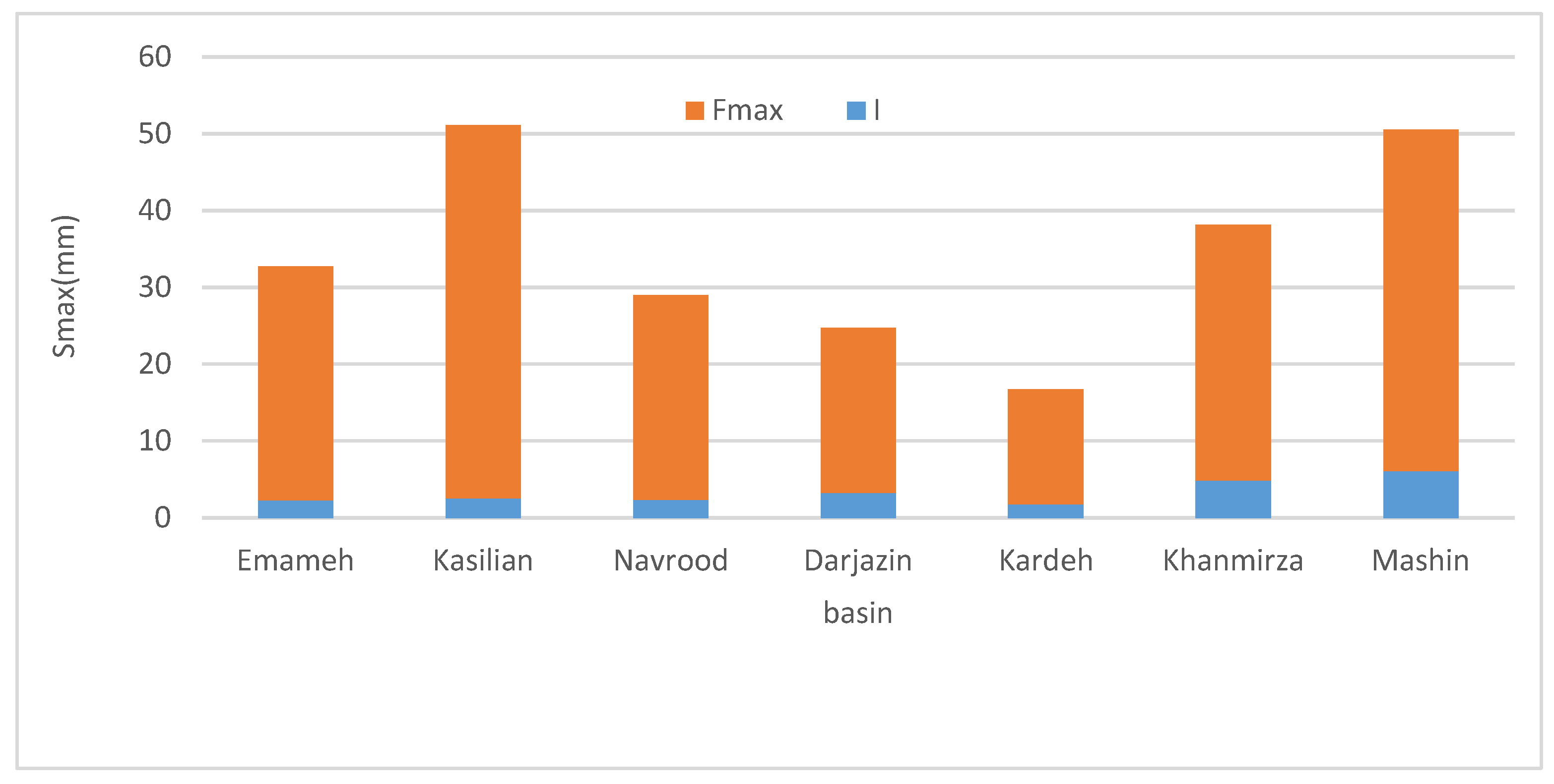
Figure 6 shows the initial storage value (I) and the potential storage, S_max (F_max + I), in the basins. The highest I is related to Mashin Basin (4.90 mm), and the lowest I is related to the Kardeh Basin (1.74 mm). Additionally, the value of I for the Kasilian Basin is equal to 2.55 mm. Although the total area of soil hydrology groups A and B (

Table 3. Soil hydrological groups for each basin (%).

Hydrological Groups	Mashin	Khanmirza	Kardeh	Darjazin	Navrood	Kasilian	Emameh
A	2.60	16.73	3.84	3.27	0.00	24.60	0.00
B	10.30	24.25	9.27	32.96	32.00	69.10	5.00
C	47.40	28.48	31.60	34.39	49.00	6.30	44.00
D	39.70	30.53	55.20	29.38	17.00	0.00	51.00

), which have more permeability, is higher in the Kasilian Basin than all the other basins (93.7%), the value of I for the Mashin Basin is higher than the I for the Kasilian Basin. This is while the Kasilian Basin does not have soil hydrology group D. Additionally, the vegetation cover of the Mashin Basin (72.8% percent) is less than that of the Kasilian (90.6%). The reason for this difference is that the value of I is mainly related to the surface absorption of soil and plants, and a part of this is used to fill the impoundments in the basin.

As a result, the deep infiltration factor does not play a big role, but the evaporation and drainage factor plays a greater role in maintaining and preventing flooding. The area of the Mashin Basin is 13 times the area of the Kasilian Basin; on the other hand, the average air temperature in the warm areas of the Mashin Basin, which plays a large role in the model results [30], is much higher than the temperature of the Kasilian Basin. Therefore, in the area of the Mashin Basin, the water flow needs more time to reach the outlet. It is noteworthy that the slope of the Mashin Basin (7.3%) is much less than the slope of the Kasilian Basin (15.8%). Therefore, there is much more time for the evaporation of surface moisture in this basin. On the other hand, in large basins, the number of surface impoundments (i.e., pools, wells, streams, etc.) is more than in small basins.

Under these conditions, it is necessary to have more rainfall in the Mashin Basin so that the flood will flow. On the contrary, in small basins with a high slope, floods occur with a small amount of precipitation. For a better understanding of this issue, we compared the S_max values of these two basins. As seen in Figure 6, the S_max value in the Mashin Basin is 50.6 mm and is about 1% less than the S_max value in the Kasilian Basin. The value for S_max in the studies of [24] is 59.2 mm for the Mashin Basin.

Therefore, although a part of S_max is related to I, deep infiltration (F_max) has a greater contribution to maximum retention (S_max). For this reason, the permeability of soil (Table 3) and vegetation cover (

Table 4. The land use in the basins (%).

Land Use	Mashin	Khanmirza	Kardeh	Darjazin	Navrood	Kasilian	Emameh
Rocky lands	16.99	0.00	68.53	47.87	0.00	8.2	0.00
Pasture	35.84	20.44	15.16	45.23	33.30	7.30	62.65
Forest	9.21	0.00	0.00	0.00	66.70	77.20	0.00
Agricultural	12.5	65.67	3.10	4.45	0.00	6.10	2.36
Residential and River	6.58	5.41	2.53	2.45	0.00	1.20	0.00
Rainfed	14.63	8.47	10.67	0.00	0.00	0.00	0.00
Wasteland	4.25	0.00	0.00	0.00	0.00	0.00	0.00

), which is higher in the Kasilian Basin than the other basins, has a greater contribution to F_max and, consequently, to the potential retention. These results clearly show that there is no significant relationship between I and S_max. This also challenges the hypothesis of SCS-CN [17] in terms of the coefficient λ (I/S_max). In other words, I is more influenced by slopes, air temperature, and impoundments, and F_max is more influenced by soil hydrological groups, vegetation cover, and impoundments. If the impoundments are very small, they will not play a role in the secondary retention value (F_max), but if the impoundments are large, they play an important role in all three retentions, I, F_max, and finally, S_max (which is the sum of all retentions).

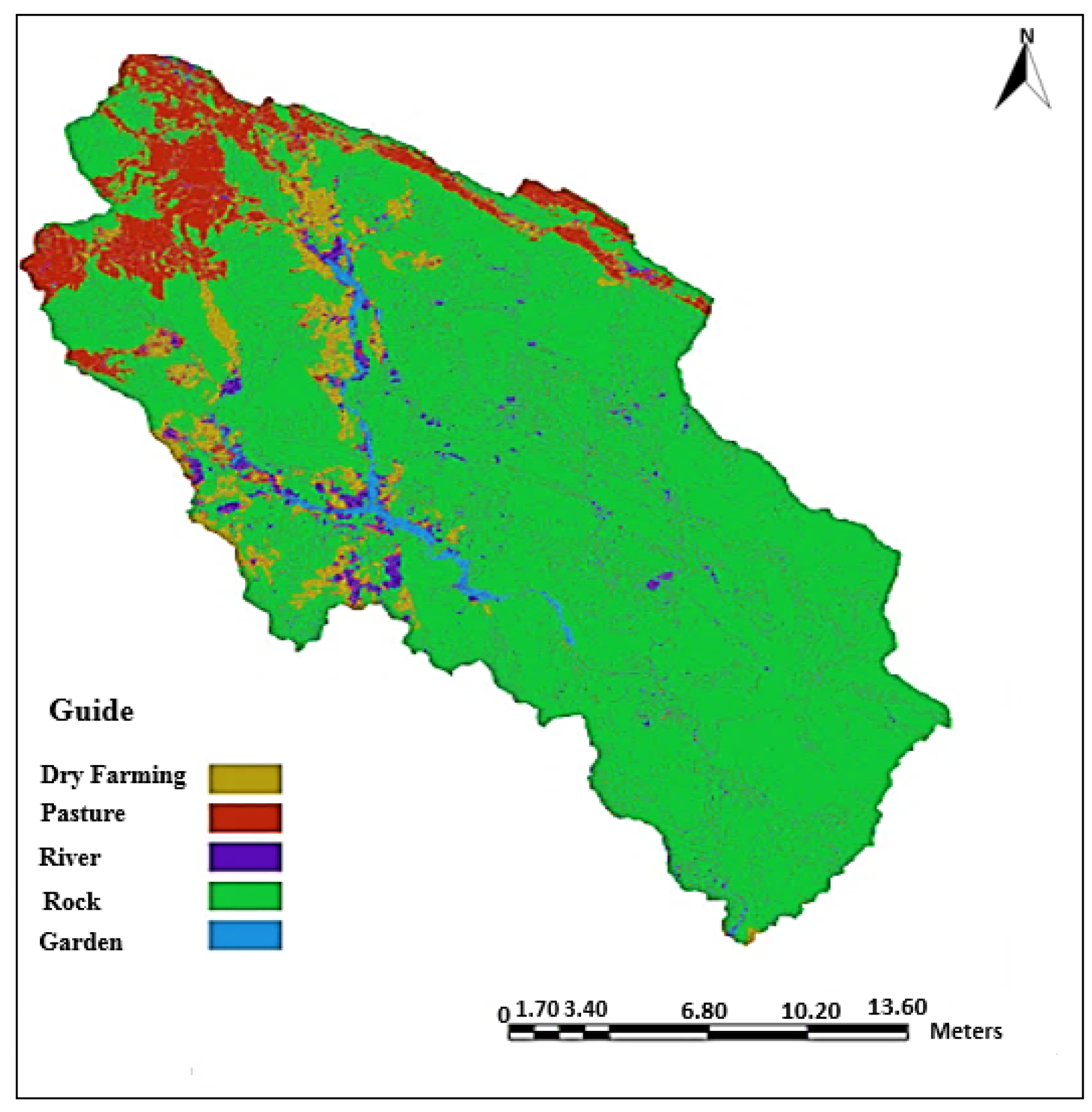
The lowest retention values (I = 1.74 mm), F_max (14.97 mm), and S_max (16.72 mm) are related to the Kardeh Basin (Figure 6); its area (547 square kilometers) is relatively large, and the slope of the basin (7.67%) is low. Therefore, it is expected that the value of I is high in the Kardeh Basin. The reason for the low retention in the Kardeh Basin is related to the soil hydrological groups and land use: when 55.2% of the basin is rocky (Group D) and the sum of groups C and D is equal to 86.8%, the impoundments are also greatly reduced, and floods will flow even with little rainfall. In other words, the value of I becomes much less than the other basins. On the other hand, the deep infiltration is also greatly reduced, and, as a result, F_max and S_max are also reduced. Figure 7 also shows the land use of the Kardeh Basin.

According to the calibration of model (10) and total retention (St),

Table 5. Results of Shamohammadi model fitting regarding the rainfall-runoff data of the Emameh, Kasilian, Navrood, Darjazin, Kardeh, Khanmirza, and Mashin basins.

Basin	$\mathit{\lambda }$	I (mm)	Model (13)
Emameh	0.07	2.3	$Q=Pa-\left(\frac{32.7Pa}{30.4+Pa}\right)$
Kasilian	0.05	2.5	$Q=Pa-\left(\frac{51.1Pa}{48.6+Pa}\right)$
Navrood	0.08	2.4	$Q=Pa-\left(\frac{29.1Pa}{26.7+Pa}\right)$
Darjazin	0.10	3.2	$Q=Pa-\left(\frac{24.7Pa}{21.5+Pa}\right)$
Kardeh	0.10	1.7	$Q=Pa-\left(\frac{16.7Pa}{14.97+Pa}\right)$
Khanmirza	0.07	2.5	$Q=Pa-\left(\frac{38.1Pa}{33.2+Pa}\right)$
Mashin	0.10	4.9	$Q=Pa-\left(\frac{50.6Pa}{44.5+Pa}\right)$

is adjusted based on the runoff-rainfall model (11).

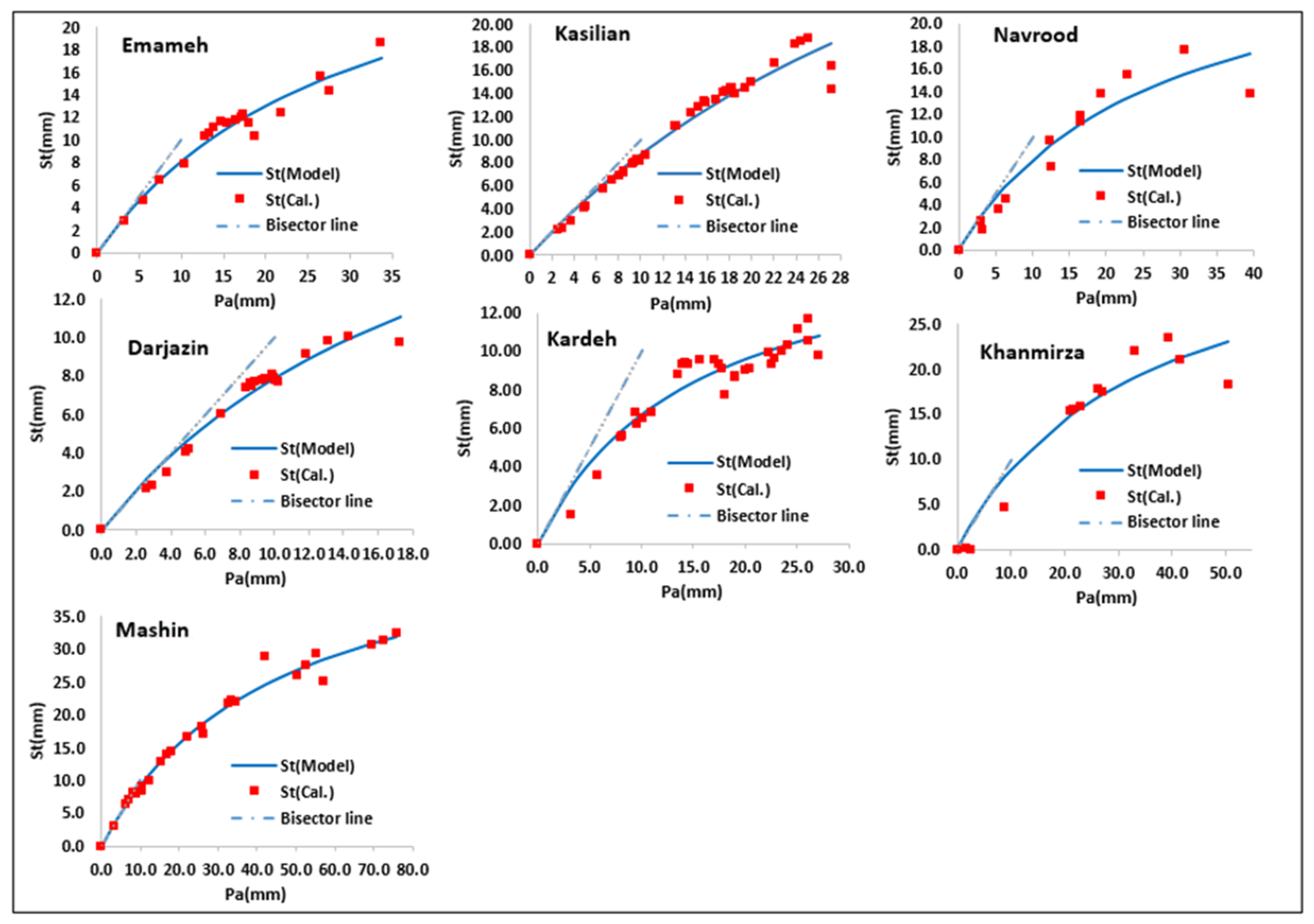
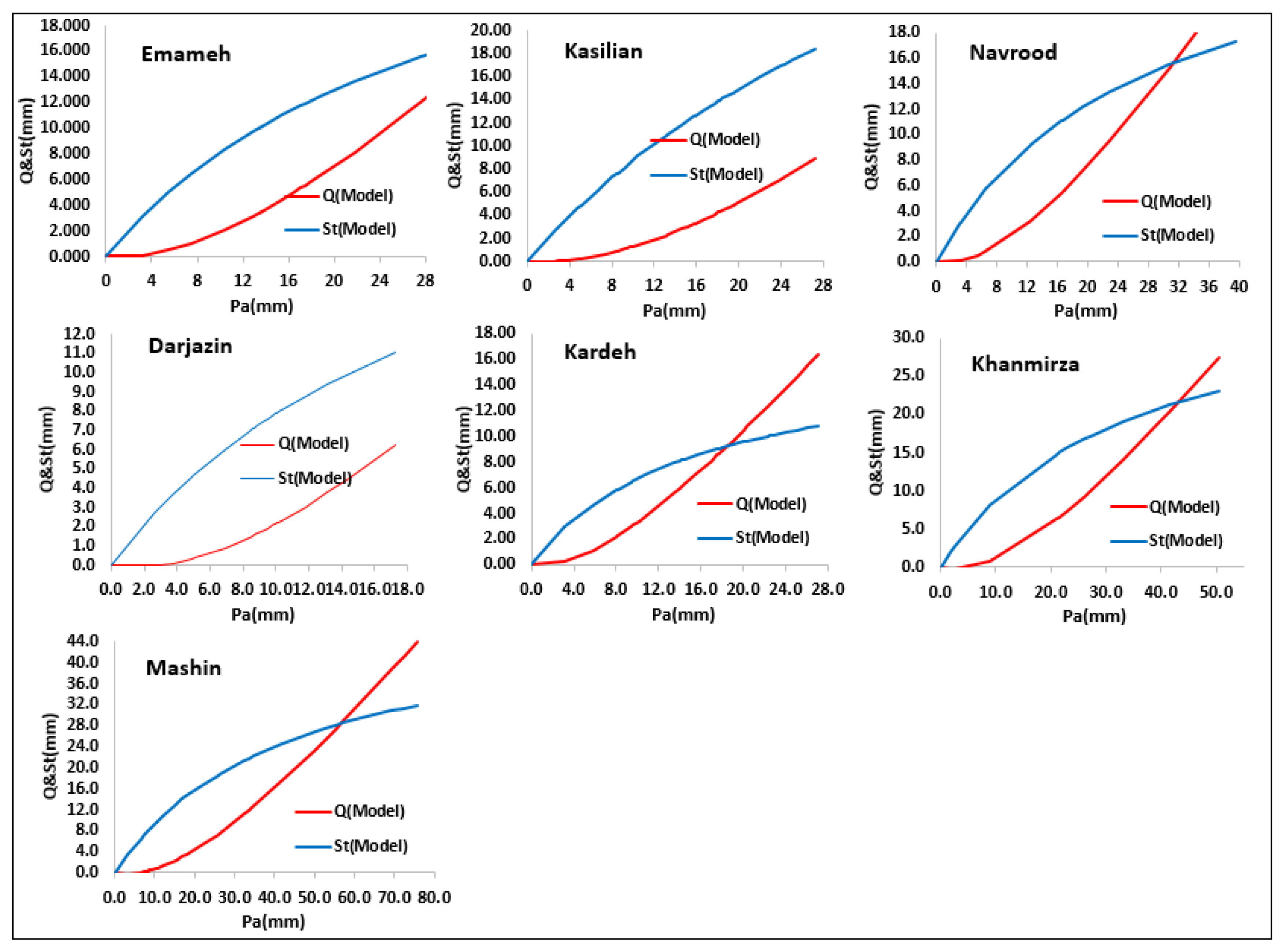
Figure 8 shows the fitting of the total retention model (S_t) to the rainfall data for the Imamah, Kasilian, Navrood, Darjazin, Kardeh, Khanmirza, and Mashin basins. As can be seen, with the increase in the amount of precipitation (P_a), the total retention slope line ($\frac{d{S}_t}{d\left(p_a\right)}$) decreases so that, at the beginning of runoff, the retention slope line from one (slope line of 45 degrees) gradually starts to decrease until P_a tends to infinity. In this case, the retention slope line also approaches zero (the retention value has reached its maximum and remains constant, Equation (10)).

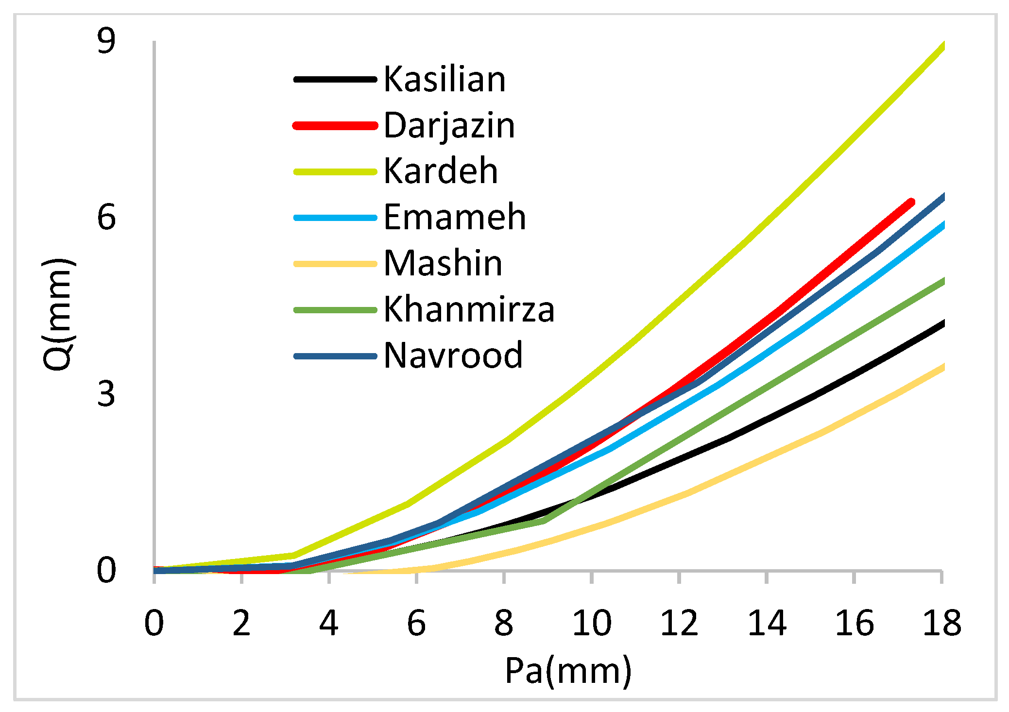
The comparison of rainfall-runoff curves in Figure 9 shows that the slope of the runoff in all basins is zero at first (P_a = I) and then gradually increases until it finally reaches 1. For a rainfall equal to P_a, the lowest value of I, the highest amount of runoff, and the highest slope line of runoff depth ($\frac{dQ}{d\left(p_a\right)}$) are related to the Kardeh Basin. As was said before, the reason for the lack of retention in the Kardeh Basin is related to the soil hydrological groups and land use [26]. Additionally, the lowest slope line is related to the Kasilian Basin. In the Kasilian Basin, due to land use (77% forest cover), secondary retention is higher than in the other basins and causes a decrease in the runoff slope line ($\frac{dQ}{d\left(p_a\right)}$).

In Figure 10, the total retention slope line ($\frac{d{S}_t}{d\left(p_a\right)}$) and runoff slope line ($\frac{dQ}{d\left(p_a\right)}$), with respect to rainfall changes, are shown. At the beginning of a rainfall event, there is no runoff (all rainfall is kept by infiltration, surface absorption, impoundments, and evaporation), and the slope line of the total retention is one ($\frac{d{S}_t}{d\left(p_a\right)}=1$). In fact, the runoff slope is equal to 0 ($\frac{dQ}{d\left(p_a\right)}=0$), while the retention slope is equal to 1. Further, with an increase in rainfall, the slope of the runoff increases, while, correspondingly, the slope of the retention decreases so that when the slope of the runoff tends to 1, the slope of the retention becomes 0. In other words, the sum of the runoff slope and retention slope is always equal to 1 (Equation (7)). These results are consistent with the results of [26].

The model evaluation results are shown in

Table 6. Evaluation results of the modified 3RM model.

Basin	NS	RMSE (mm)	R2
Emameh	0.96	0.86	0.96
Kasilian	0.94	0.93	0.86
Navrood	0.78	1.1	0.78
Darjazin	0.79	0.89	0.79
Kardeh	0.96	0.89	0.87
Khanmirza	0.90	2.28	0.84
Mashin	0.91	1.42	0.88

. As can be seen, the coefficient of determination (R²) for predicting runoff was between 0.78 and 0.96 in the Navrood and Darjazin basins, respectively, and are within an acceptable range. The root mean square errors (RMSEs) are also between 0.86 and 2.28, and the Nash–Sutcliffe efficiency (NSE) varied between 0.79 and 0.96, which are within the significant range.

4. Conclusions and Results

• In this study, it was shown that the amount of primary retention (I) is more influenced by the slope of the basin, air temperature, and impoundment. While the secondary retention (F_max) is more influenced by the soil hydrological group, vegetation cover, and impoundment. If the impoundments are very small, they will not play a role in the secondary retention value, but if the impoundments are large and deep, they play an important role in all three retentions (I, F_max, and S_max);
• Unlike the models that have fixed coefficients, in this model, all the parameters, including P_a, I, F_max, and S_max, are defined. For this reason, the model has high sensitivity;
• In the present model, the method of estimating the parameters (I, F_max, and S_max) is completely different from the SCS-CN method and can be easily calculated;
• The results of fitting the model to the rainfall-runoff data based on R², RMSE, and NS showed that the model has an acceptable ability to predict runoff and retention in all studied basins, especially if the selection of rainfall-runoff data was carried out carefully. In any case, if the rainfall-runoff data are consistent with the conceptual rainfall–runoff curve, we can expect very good results;
• The new model is completely consistent with the revised SCS-CN conceptual curve, but its mathematical model is different from the SCS-CN mathematical model (the SCS-CN model does not have boundary conditions ($\underset{{\mathrm{P}}_{\mathrm{a}}\to 0}{\mathit{lim}}\left(\mathrm{Q}\right)\ne 0$)).