
Separation of Floodplain Flow and Bankfull Discharge: Application of 1D Momentum Equation Solver and MIKE 21C

Abstract
:1. Introduction
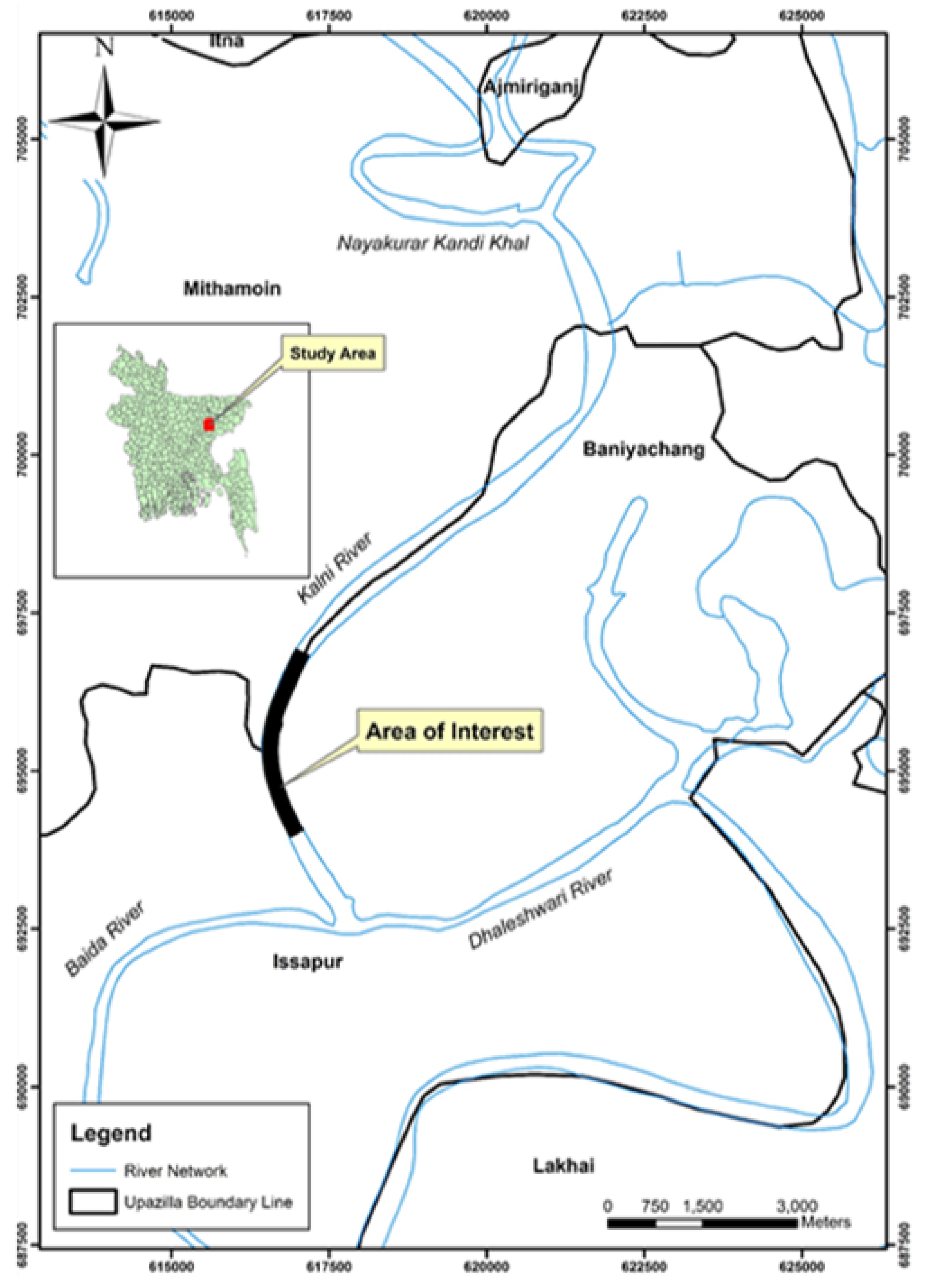
2. Study Area
3. Methods
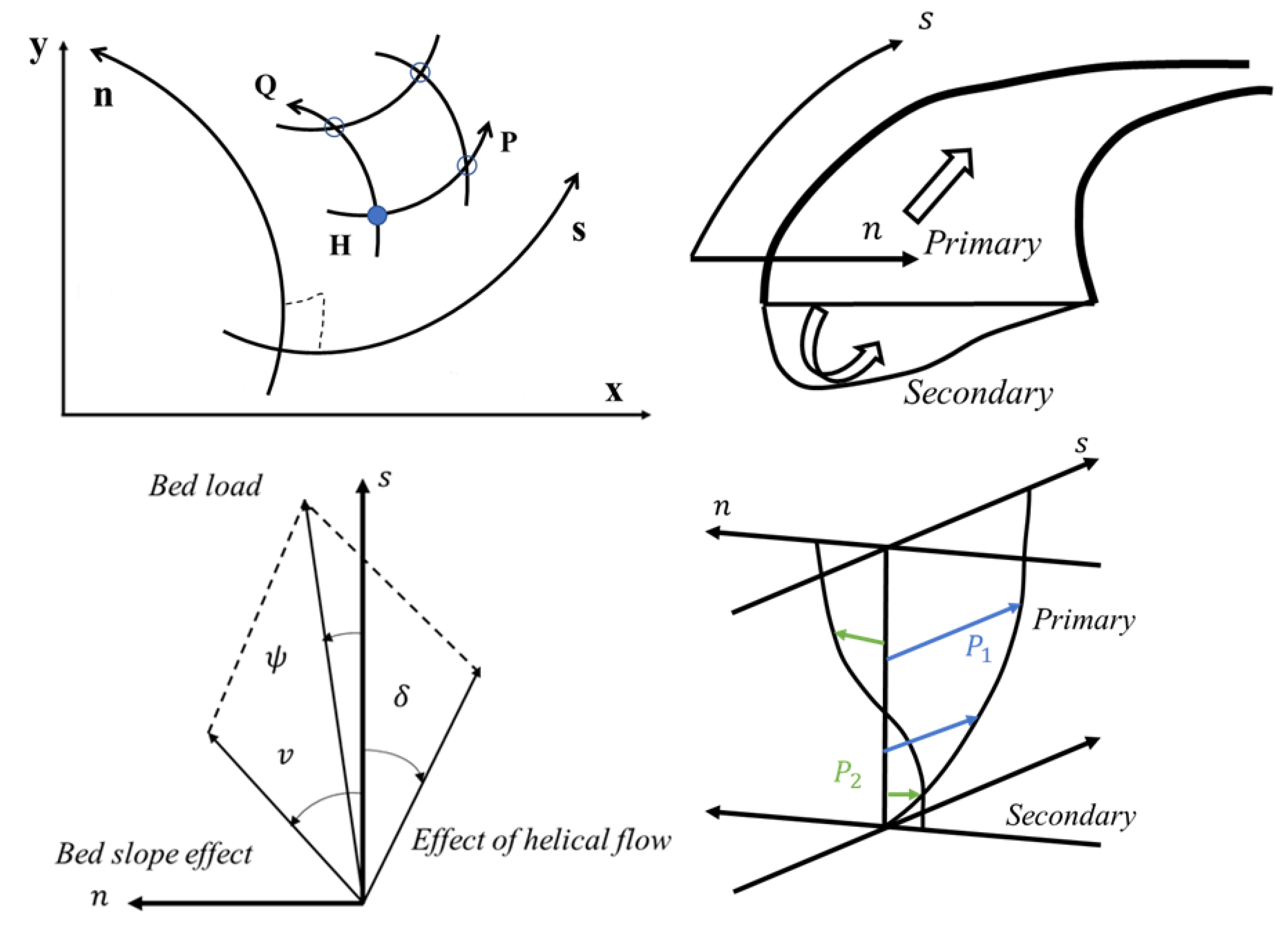
3.1. One-Dimensional Governing Equation
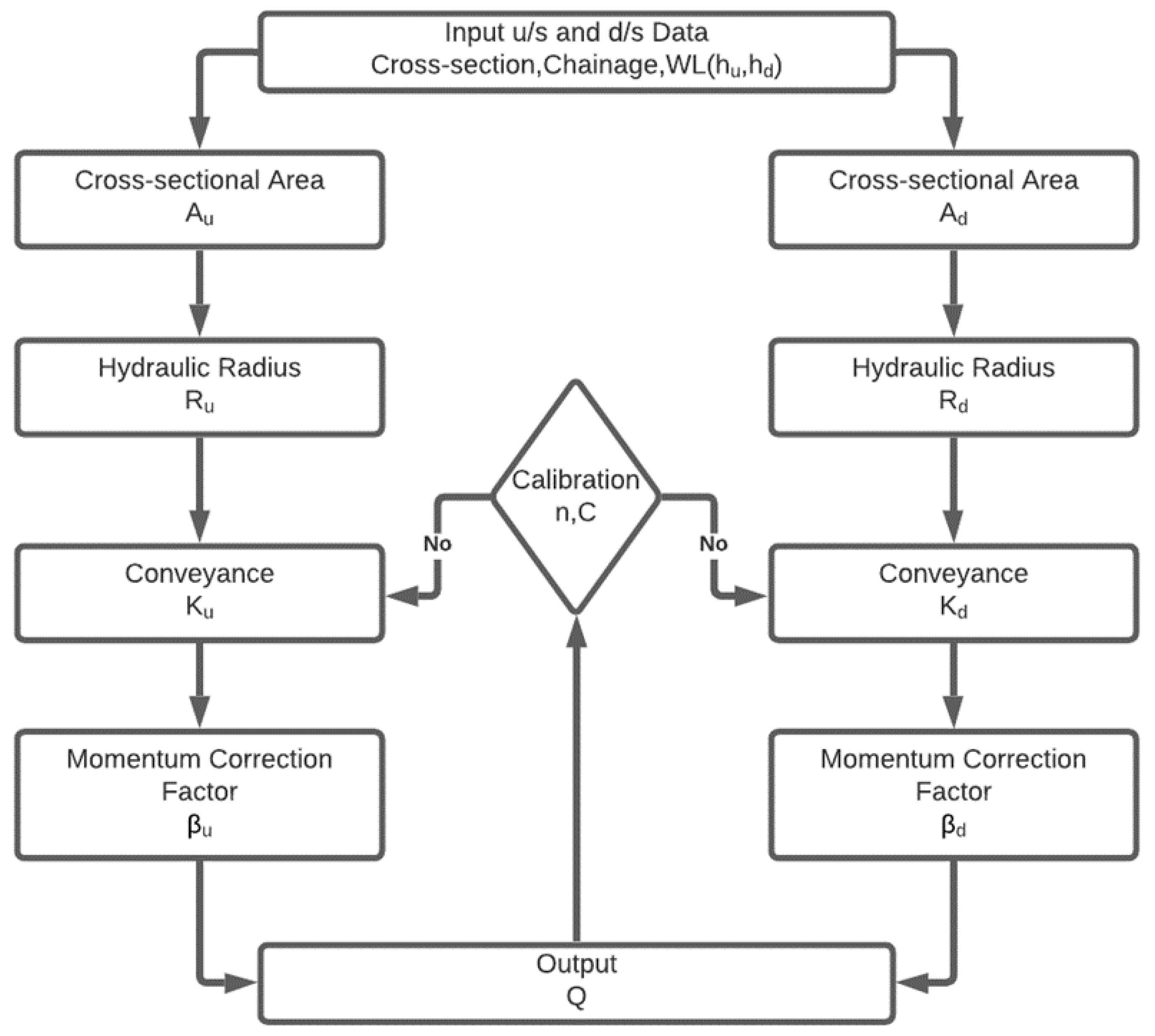
3.2. Solution of the 1D Governing Equation
3.3. MIKE 21C Curvilinear Model
3.3.1. Curvilinear Grid Generator
3.3.2. Two-Dimensional Hydrodynamic Model
3.3.3. Sediment Transport
3.3.4. Morphology
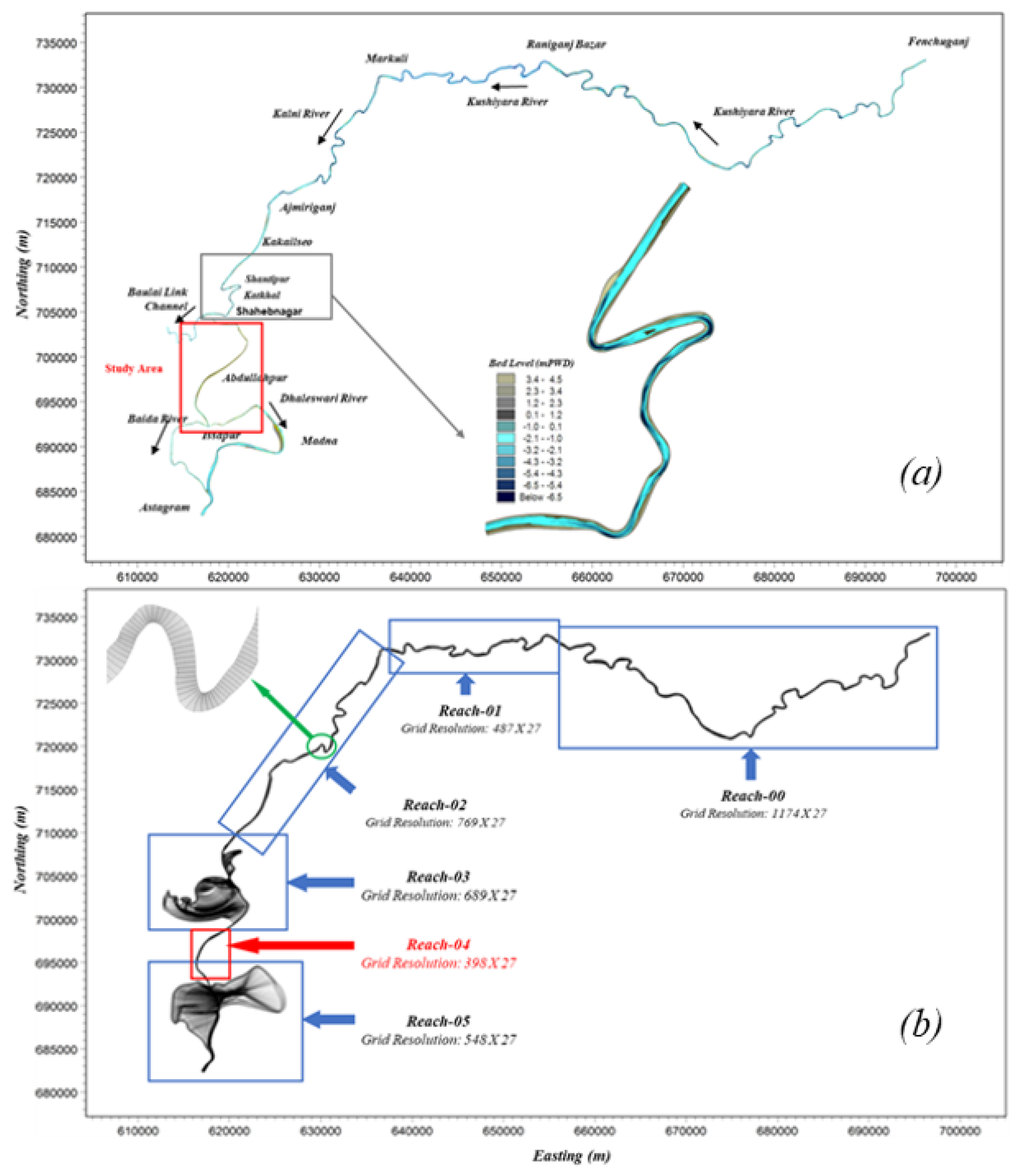
3.4. MIKE 21C Curvilinear Model Setup
4. Input Data
5. Results and Discussion
6. Conclusions and Recommendation
Funding
Institutional Review Board Statement
Informed Consent Statement
Data Availability Statement
Acknowledgments
Conflicts of Interest
References
- Goudie, A. Encyclopedia of Geomorphology; Springer: Berlin, Germany, 2004; Volume 2. [Google Scholar]
- Sarker, S.; Veremyev, A.; Boginski, V.; Singh, A. Critical nodes in river networks. Sci. Rep. 2019, 9, 11178. [Google Scholar] [CrossRef] [PubMed]
- Sarker, S. Investigating Topologic and Geometric Properties of Synthetic and Natural River Networks under Changing Climate. Ph.D. Thesis, University of Central Florida, Orange County, FL, USA, 2021. [Google Scholar]
- Gao, Y.; Sarker, S.; Sarker, T.; Leta, O.T. Analyzing the critical locations in response of constructed and planned dams on the Mekong River Basin for environmental integrity. Environ. Res. Commun. 2022, 4, 101001. [Google Scholar] [CrossRef]
- Copeland, R.R.; McComas, D.N.; Thorne, C.R.; Soar, P.J.; Jonas, M.M. Hydraulic design of stream restoration projects. In Engineer Research and Development Center Vicksburg ms Coastal and Hydraulicslab; Technical Report; US Army Corps of Engineers, Engineer Research and Development Center: Vicksburg, MI, USA, 2001. [Google Scholar]
- Andrews, E.D. Effective and bankfull discharges of streams in the Yampa River basin, Colorado and Wyoming. J. Hydrol. 1980, 46, 311–330. [Google Scholar] [CrossRef]
- Biedenharn, D.S.; Copeland, R.R.; Thorne, C.R.; Soar, P.J.; Hey, R.D.; Watson, C.C. Effective Discharge Calculation: A Practical Guide; US Army Corps of Engineers, Engineer Research and Development Center: Vicksburg, MI, USA, 2000.
- Boyd, K.; Doyle, M.; Rotar, M.; Bathala, C. Estimation of dominant discharge in an unstable channel environment. In Proceedings of the 1999 International Water Resources Engineering Conference, Reston, VA, USA, 1999; Available online: http://www.extranet.vdot.state.va.us/locdes/hydraulic_design/nchrp_rpt544/content/html/Special_Topics/Bankfull_Discharge.html (accessed on 8 August 2013).
- Doyle, M.W.; Boyd, K.F.; Skidmore, P.B. River restoration channel design: Back to the basics of dominant discharge. In Proceedings of the 2nd International Conference on National Channel Systems, Ministry of Natural Resources, Petersborough, ON, Canada, 1–4 March 1999. [Google Scholar]
- Emmett, W.W.; Wolman, M.G. Effective discharge and gravel-bed rivers. Earth Surf. Process. Landf. 2001, 26, 1369–1380. [Google Scholar] [CrossRef]
- Federal Interagency Stream Restoration Working Group. Stream Corridor Restoration: Principles, Processes, and Practices; U.S. Department of Commerce: Springfield, VI, USA, 1998.
- Hey, R. Design discharge for natural channels. In Science, Technology and Environmental Management; Hey, R.D., Davies, T.D., Eds.; Saxon House: Farnborough, UK, 1975; pp. 73–88. [Google Scholar]
- Hey, R. Restoration of gravel-bed rivers: Principles and practice. In Natural Channel Design: Perspectives and Practice; Canadian Water Resources Association: Cambridge, ON, Canada, 1994; pp. 157–173. [Google Scholar]
- Jennings, M.E.; Thomas, W.O.; Riggs, H. Nationwide Summary of US Geological Survey Regional Regression Equations for Estimating Magnitude and Frequency of Floods for Ungaged Sites, 1993; USGS: Reston, VI, USA, 1994.
- Kondolf, G.M.; Smeltzer, M.W.; Railsback, S.F. Design and performance of a channel reconstruction project in a coastal California gravel-bed stream. Environ. Manag. 2001, 28, 761–776. [Google Scholar] [CrossRef]
- Ministry of Natural Resources. Natural Channel Systems: An Approach to Management and Design, Queen’s Printer for Canada, Toronto; Ministry of Natural Resources: Toronto, ON, Canada, 1994.
- Pickup, G. Adjustment of stream-channel shape to hydrologic regime. J. Hydrol. 1976, 30, 365–373. [Google Scholar] [CrossRef]
- Racin, J.A.; Hoover, T.P.; Crossett Avila, C.M. California Bank and Shore Rock Slope Protection Design: Practitioner’s Guide and Field Evaluations of Riprap Methods; Technical Report; California Department of Transportation: Sacramento, CA, USA, 2000.
- Riley, A.L. Restoring Streams in Cities; Island Press: Washington, DC, USA, 1998. [Google Scholar]
- Rosgen, D.L. Applied River Morphology; Wildland Hydrology: Fort Collins, CO, USA, 1996. [Google Scholar]
- Schumm, S.A.; Harvey, M.D.; Watson, C.C. Incised Channels: Morphology, Dynamics, and Control; Water Resources Publications: Seattle, WA, USA, 1984. [Google Scholar]
- Simon, A. The discharge of sediment in channelized alluvial streams 1. JAWRA J. Am. Water Resour. Assoc. 1989, 25, 1177–1188. [Google Scholar] [CrossRef]
- Soar, P.; Thorne, C. Channel Restoration Design for Meandering Rivers; ERDC/ CHL CR-01-1; US Army Engineer Research and Development Center, Flood Damage Reduction Research Program: Vicksburg, MI, USA, 2001.
- Thorne, C.R.; Allen, R.G.; Simon, A. Geomorphological river channel reconnaissance for river analysis, engineering and management. Trans. Inst. Br. Geogr. 1996, 21, 469–483. [Google Scholar] [CrossRef]
- Watson, C.; Dubler, D.; Abt, S. Demonstration Erosion Control Project Report: Design Hydrology Investigations; River and Streams Studies Center, Colorado State University: Fort Collins, CO, USA, 1997. [Google Scholar]
- Wharton, G.; Arnell, N.; Gregory, K.; Gurnell, A. River discharge estimated from channel dimensions. J. Hydrol. 1989, 106, 365–376. [Google Scholar] [CrossRef]
- Wolman, M.G.; Miller, J.P. Magnitude and frequency of forces in geomorphic processes. J. Geol. 1960, 68, 54–74. [Google Scholar] [CrossRef]
- Williams, G.P. Bank-full discharge of rivers. Water Resour. Res. 1978, 14, 1141–1154. [Google Scholar] [CrossRef]
- Dottori, F.; Martina, M.; Todini, E. A dynamic rating curve approach to indirect discharge measurement. Hydrol. Earth Syst. Sci. 2009, 13, 847–863. [Google Scholar] [CrossRef]
- Koussis, A. Comment on “A dynamic rating curve approach to indirect discharge measurement” by Dottori et al. (2009). Hydrol. Earth Syst. Sci. 2009, 14, 1093–1097. [Google Scholar] [CrossRef]
- Reitan, T.; Petersen-Øverleir, A. Dynamic rating curve assessment in unstable rivers using Ornstein-Uhlenbeck processes. Water Resour. Res. 2011, 47. [Google Scholar] [CrossRef]
- Morlot, T.; Perret, C.; Favre, A.C.; Jalbert, J. Dynamic rating curve assessment for hydrometric stations and computation of the associated uncertainties: Quality and station management indicators. J. Hydrol. 2014, 517, 173–186. [Google Scholar] [CrossRef]
- Sarker, S. Hydraulics Lab Manual. engrXiv 2021, 1–66. [Google Scholar] [CrossRef]
- Sarker, S. A Short Review on Computational Hydraulics in the context of Water Resources Engineering. Open J. Model. Simul. 2022, 10, 1–31. [Google Scholar] [CrossRef]
- Sarker, S. Pipe Network Design and Analysis: An Example with WaterCAD. engrXiv 2021. [Google Scholar] [CrossRef]
- Schumm, S.A. The Fluvial System; Wiley: New York, NY, USA, 1977; p. 338. [Google Scholar] [CrossRef]
- Womack, W.; Schumm, S. Terraces of Douglas Creek, northwestern Colorado: An example of episodic erosion. Geology 1977, 5, 72–76. [Google Scholar] [CrossRef]
- Montgomery, D.R.; Buffington, J.M. Channel-reach morphology in mountain drainage basins. Geol. Soc. Am. Bull. 1997, 109, 596–611. [Google Scholar] [CrossRef]
- Buffington, J.M.; Montgomery, D.R. A systematic analysis of eight decades of incipient motion studies, with special reference to gravel-bedded rivers. Water Resour. Res. 1997, 33, 1993–2029. [Google Scholar] [CrossRef]
- Dutta, D.; Alam, J.; Umeda, K.; Hayashi, M.; Hironaka, S. A two-dimensional hydrodynamic model for flood inundation simulation: A case study in the lower Mekong river basin. Hydrol. Process. Int. J. 2007, 21, 1223–1237. [Google Scholar] [CrossRef]
- Sarker, S.; Sarker, T.; Leta, O.T.; Raihan, S.U.; Khan, I.; Ahmed, N. Understanding the Planform Complexity and Morphodynamic Properties of Brahmaputra River in Bangladesh: Protection and Exploitation of Riparian Areas. Water 2023, 15, 1384. [Google Scholar] [CrossRef]
- Reza, A.A.; Sarker, S.; Asha, S.A. An Application of 1-D Momentum Equation to Calculate Discharge in Tidal River: A Case Study on Kaliganga River. Tech. J. River Res. Inst. 2014, 2, 77–86. [Google Scholar]
- Sarker, S.; Sarker, T. Spectral Properties of Water Hammer Wave. Appl. Mech. 2022, 3, 799–814. [Google Scholar] [CrossRef]
- Sarker, S. Essence of MIKE 21C (FDM Numerical Scheme): Application on the River Morphology of Bangladesh. Open J. Model. Simul. 2022, 10, 88–117. [Google Scholar] [CrossRef]
- Danish Hydraulic Institute (DHI). MIKE 21C, Curvilinear Model—Scientific Documentation. Available online: https://manuals.mikepoweredbydhi.help/2017/Water_Resources/MIKE21C_Scientific_documentation.pdf (accessed on 25 November 2017).
- Sarker, S. Fundamentals of Climatology for Engineers: Lecture Note. Eng 2022, 3, 573–595. [Google Scholar] [CrossRef]


| Statistic | MIKE 21C (Daily) | Simulated (Daily) | MIKE 21C (Monthly) | Simulated (Monthly) |
|---|---|---|---|---|
| Count | 2913 | 2916 | 12 | 12 |
| Mean | 49.79 | 50.88 | 49.44 | 50.56 |
| Std | 44.82 | 48.54 | 45.38 | 49.07 |
| Min | 1.56 | 0.52 | 3.91 | 2.17 |
| 25% | 7.06 | 4.48 | 7.93 | 5.10 |
| 50% | 32.37 | 30.88 | 35.87 | 35.42 |
| 75% | 97.92 | 103.36 | 96.05 | 99.09 |
| Max | 124.67 | 131.67 | 110.21 | 120.55 |
| Statistic Comparison | Daily Comparison | Monthly Comparison | ||
| Mean error or bias | 1.14 | 1.12 | ||
| Percent bias | 2.29 | 2.27 | ||
| Absolute percent bias | 7.39 | 6.55 | ||
| Root-mean-square error (RMSE) | 4.77 | 4.26 | ||
| Centered RMSD (CRMSD) | 4.64 | 4.12 | ||
| Pearson correlation coefficient (r) | 0.99 | 0.99 | ||
| Coefficient of determination () | 0.99 | 0.99 | ||
| Skill score (Murphy) | 0.98 | 0.99 | ||
| Nash–Sutcliffe efficiency | 0.98 | 0.99 | ||
| Kling–Gupta efficiency (2009) | 0.91 | 0.91 | ||
| Kling–Gupta efficiency (2012) | 0.93 | 0.93 | ||
| Index of agreement | 0.99 | 0.99 | ||
| Brier’s score | 3772.54 | 15.10 | ||
| Mean absolute error | 3.68 | 3.23 | ||
| Common count | 2913 | 12 | ||
| Count of NaNs | 3 | 0 | ||
| Mean | 49.79 | 49.43 | ||
| Standard deviation | 44.826 | 45.38 | ||
Disclaimer/Publisher’s Note: The statements, opinions and data contained in all publications are solely those of the individual author(s) and contributor(s) and not of MDPI and/or the editor(s). MDPI and/or the editor(s) disclaim responsibility for any injury to people or property resulting from any ideas, methods, instructions or products referred to in the content. |
© 2023 by the author. Licensee MDPI, Basel, Switzerland. This article is an open access article distributed under the terms and conditions of the Creative Commons Attribution (CC BY) license (https://creativecommons.org/licenses/by/4.0/).
Share and Cite
Sarker, S. Separation of Floodplain Flow and Bankfull Discharge: Application of 1D Momentum Equation Solver and MIKE 21C. CivilEng 2023, 4, 933-948. https://doi.org/10.3390/civileng4030050
Sarker S. Separation of Floodplain Flow and Bankfull Discharge: Application of 1D Momentum Equation Solver and MIKE 21C. CivilEng. 2023; 4(3):933-948. https://doi.org/10.3390/civileng4030050
Chicago/Turabian StyleSarker, Shiblu. 2023. "Separation of Floodplain Flow and Bankfull Discharge: Application of 1D Momentum Equation Solver and MIKE 21C" CivilEng 4, no. 3: 933-948. https://doi.org/10.3390/civileng4030050