Nonlinear Dynamic Analyses Utilising Macro-Models of Reinforced Concrete Building Structures and Site-Specific Accelerograms

Abstract

This paper aims to guide structural engineers on how to apply the rapid nonlinear time history analysis (RNLTHA) procedure effectively to predict seismic demand, taking into account ductility and overstrength, and effects of dynamic phenomena including cyclic degradation of strength and stiffness in structures, in a direct and expedient manner. The shortcoming of the conventional force-based approach of design involving the use of a force reduction factor to account for nonlinear effects is well recognised. Nonlinear static (pushover) analysis and dynamic nonlinear time history analysis (NLTHA) are offered as alternative methods of analysis by major codes of practices to achieve better optimisation in the use of materials. NLTHA has advantages over pushover analysis in being more direct and capable of capturing cyclic response behaviour. Despite the merits of NLTHA, its adoption in the industry has been limited, mainly because of the complexity and the higher analysis cost involved. RNLTHA proposed in this article uses a macroscopic model of the building to fulfil the purpose of NLTHA, whilst saving computational time and achieving a good degree of accuracy, as verified by comparison with results generated from SeismoStruct.

1. Introduction

The earthquake-resisting design of a building structure involves the use of efficient computational tools to give an estimate of seismic demand, taking into account dynamic actions. Current codes of practice typically stipulate prescriptive design procedures employing force-based design principles for ensuring satisfactory performance of the structure in countering seismic actions. Traditionally, the linear elastic behaviour of the structure is assumed in analysis for determining internal forces sustained by the structural element. A force reduction factor (which is also known as the behaviour factor, performance factor or structural response factor) is then applied to the internal forces in the building to take into account the effects of ductility and overstrength. The main shortcoming of this (widely adopted) approach to structural design for seismic action is the inability of the force reduction factor to predict the seismic response behaviour of the structure accurately when excited beyond the limit of yield. The potential performance behaviour of the building is always in question should there be certain dominant atypical structural features in the load transmission path, despite the design being code compliant. In addressing this issue, most major codes of practice offer the option of nonlinear static or nonlinear time history (dynamic), analysis, both of which are based on fewer simplified assumptions [1,2,3,4]. The latter in particular is considered to provide better assurance of the safety and operability of the structure when subject to severe ground shaking [5]. A nonlinear analysis procedure that employs site-specific information (in the form of response spectra and/or strong motion accelerograms) as input into the analysis would also serve the purpose of achieving better optimisation of the use of materials, saving construction costs [6]. Despite the potential benefits, practising engineers tend to opt out of becoming involved in nonlinear dynamic analysis because of the effort and cost and the lack of guidance and information in support of the preparation of input into the software. The key motivation in the writing of this article is to facilitate structural designers to adopt more advanced analytical procedures through the introduction of modelling methodologies (such as macro-modelling), which consume less computational time and provide better support to guide input into the software.

Nonlinear seismic analysis of buildings may be either nonlinear static (pushover) analysis or nonlinear time history analysis (NLTHA). Pushover analysis, which is filled with limitations, can be used for calculating the resistant capacity and validation of the likely performance of the building [3,4]. It can be argued that the limitations of pushover analysis in modelling cyclic degradation can be overcome. However, the use of pushover analysis in dealing with a 3D dynamic response remains challenging. NLTHA gives predictions of the time history of drifts and internal forces, taking into account cyclic nonlinear material properties [5]. Extending NLTHA from a 2D to a 3D response is more straightforward than achieving the same with pushover analysis. Despite the considerable benefits of NLTHA, the implementation of this type of analysis is mostly restricted to use in research because of the challenges posed to structural designers. The first challenge is to do with obtaining a large enough ensemble of strong motion accelerograms that are representative of the targeted site for a given intensity of seismic hazard. In addressing this challenge, methods of generating and sorting code-compliant accelerograms on bedrock and soil surfaces have been developed [7,8,9,10] and incorporated into “quakeadvice.org” [11]. The second challenge is the high computational cost of modelling the whole building for the prediction of its dynamic behaviour throughout the duration of the response. The need to iterate over each time step in the analysis of a nonlinear system can result in a long execution time. The issue of a prolonged computation is compounded by the need to repeat the analysis with changing fineness of the meshing to demonstrate convergence [12], and to have the procedure repeated to make full use of each record in the designated accelerogram ensemble. The writing of this paper was motivated by the need to address the second challenge as described.

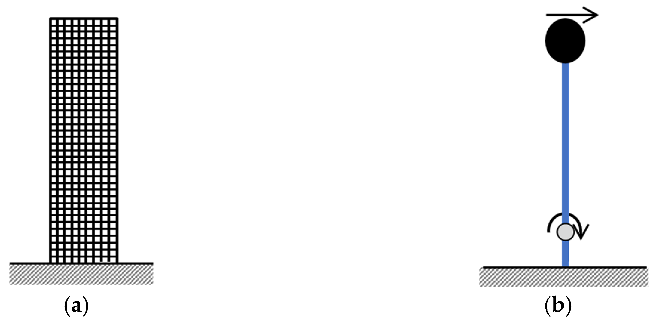
Recent analytical and experimental research has significantly improved our understanding of the inelastic behaviour of structural walls. Suitable analytical models in support of NLTHA have been developed. A macroscopic model of a structural wall providing lateral resistance to the building (abbreviated herein as a macro-model) has advantages over a conventional finite element model because of the much-reduced memory consumption and input information. The type of macro-model introduced herein is a vertical line element (a “stick”), which supports a lumped mass at the top. The stick has a hinge at the base to emulate the formation of a plastic hinge at the base of an RC wall. The proposed “rapid nonlinear time history analysis (RNLTHA)” procedure is performed on the model to give predictions of the time history response of the lumped mass. The nonlinear behaviour of the base (plastic) hinge is defined following a pre-determined moment–rotational relationship. In Figure 1, an example of a stick model (Figure 1b) for representing a shear wall is shown alongside the finite element model (Figure 1a), where the difference between the number of degrees of freedom between the two models is presented. An outline of the operational details of RNLTHA is presented in Section 2. Its application is demonstrated in Section 4 in the form of a case study, and the results are compared with the sophisticated finite element analysis. For analysing the case study building, RNLTHA algorithms were implemented using MATLAB Version R2022a [13], and SeismoStruct Version 2021 [14] was used for conducting the finite element analysis.

With tall buildings, the stick model as described would need to support multiple lumped masses (MDOF system). An outline of the operational details of RNLTHA when applied to this type of macro-model, including brief details of manipulation of the mass, stiffness and damping matrices, are presented in Section 3. Further research is planned for the implementation of RNLTHA to analyse such structures.

2. Rapid Nonlinear Time History Analysis (RNLTHA)

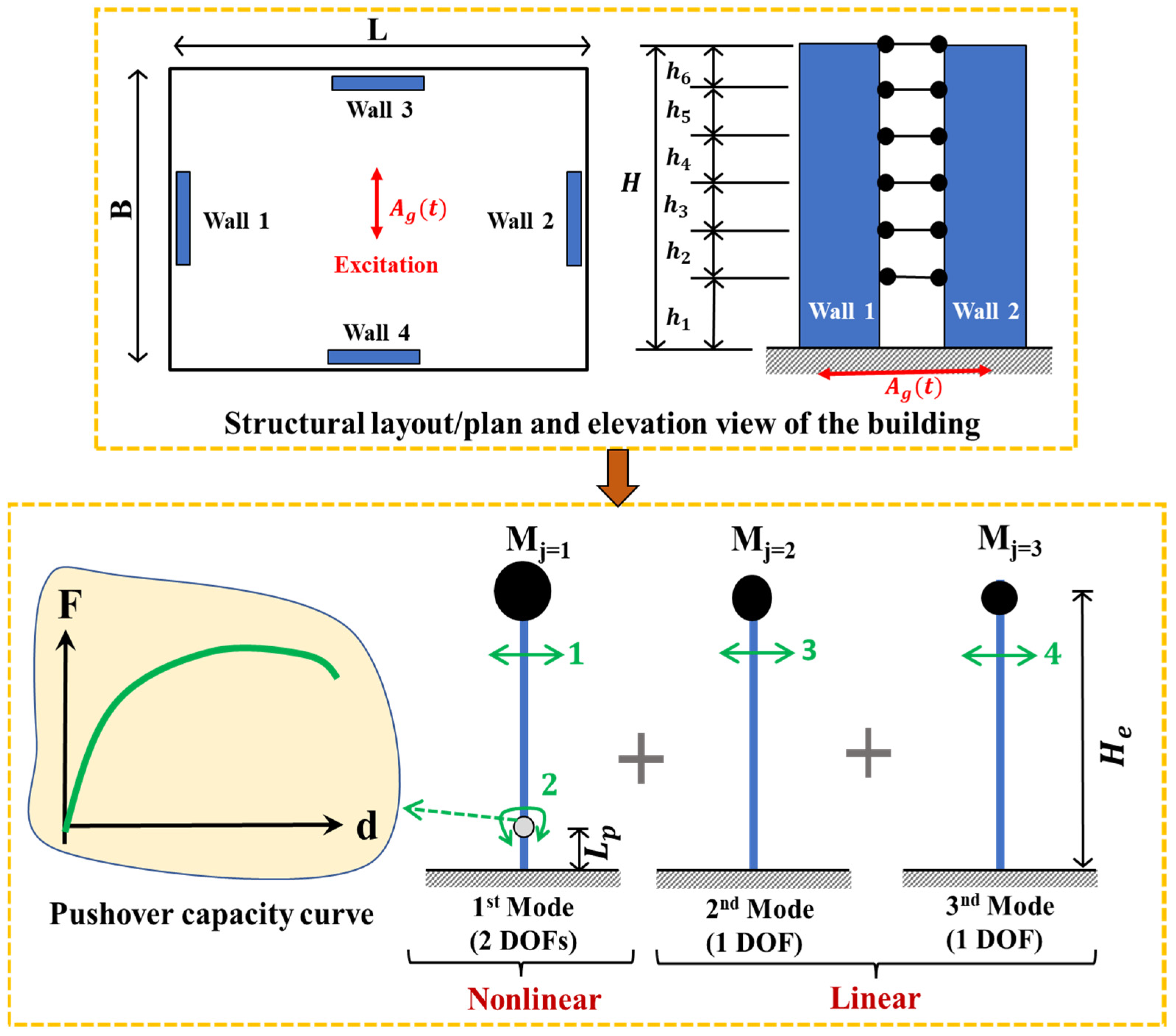
The fast-track version of nonlinear time history analysis, known as “rapid nonlinear time history analysis (RNLTHA)” for predicting the time history response of RC buildings, is based on a macroscopic model having a lumped mass at an effective height ($H_e)\cong 0.7\times$ total height [15], as shown in Figure 2. In RNLTHA, the building is subject to modal analysis to resolve the linear elastic response components into multiple modes of vibration, as is performed conventionally [3]. The nonlinear component is represented by the rotation of the “stick” about the hinge at the base to emulate the effects of plastic hinge formation. The inelastic response of the first mode and the elastic responses of the higher modes are combined to form the final solution. It is assumed that the inelastic action is mainly associated with the first mode while having a comparatively minor effect on the higher modes. This is supported by the findings presented in Refs. [16,17,18], which recommends that the ductility in an RC wall structure is largely concentrated in its first mode (however, this is not valid for buildings with a frame system providing full or partial lateral support). With this macro model, thousands of degrees of freedom in a multi-storey building are reduced to four degrees of freedom (DOFs): two for the first mode, one for the second mode and one for the third mode. The use of this feature makes RNLTHA unique compared with other existing simplified methods. Attributed to simplicity, RNLTHA is memory inexpensive and transparent, and the savings in computational time and costs are considerable. Whilst saving computational time, analyses are repeated to cover every accelerogram in the ensemble. The time step interval is also kept sufficiently short (about 0.005 s) to give robust predictions.

The RNLTHA methodology introduced in this section is limited to the determination of the 2D time history responses: displacement and storey shear of a wall-type building that can be approximated by considering four DOFs covering three modes of vibration and the assumption of a plastic hinge formed at the base of the building. A more general modelling methodology that is without these restrictions is recommended for future study. The extended modelling methodology for 3D modelling of the dynamic response, taking into account torsional actions, is introduced in RNLTHA-3D in Ref. [19].

The RNLTHA procedure involves three routines: (Routine 1) generation of two to six soil surface accelerograms for each reference period of 0.2 s, 0.5 s, 1 s and 2 s using the procedure introduced in Refs. [10,11], which has been implemented into ‘quakeadvice.org’; (Routine 2) dynamic modal analysis of the building to obtain the eigen solutions (presented in Section 2.1); and (Routine 3) conducting fast-tracked nonlinear time history analysis of the stick model, which serves the purpose of determining the time history response for a given ground motion excitation. The breakdown of Routine 3 is presented below:

Step 1: Determine the modal mass ($M_j$), angular frequency (${\omega }_{n,j}$) and displacement coefficient ($P_{n,j}$) for the first three modes of vibration (j = 1 to 3), as elaborated in Section 2.1.

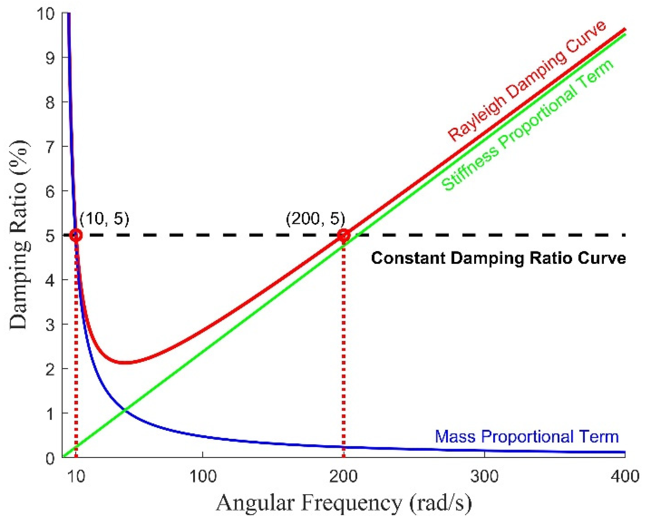
Step 2: Determine the elastic response of the SDOF for the first three modes of vibration for the current time step using Equations (A1)–(A4). The structural damping ratio ($\zeta$) of 0.05 may be used for all vibration modes, as recommended by various texts and standards [15,20,21].

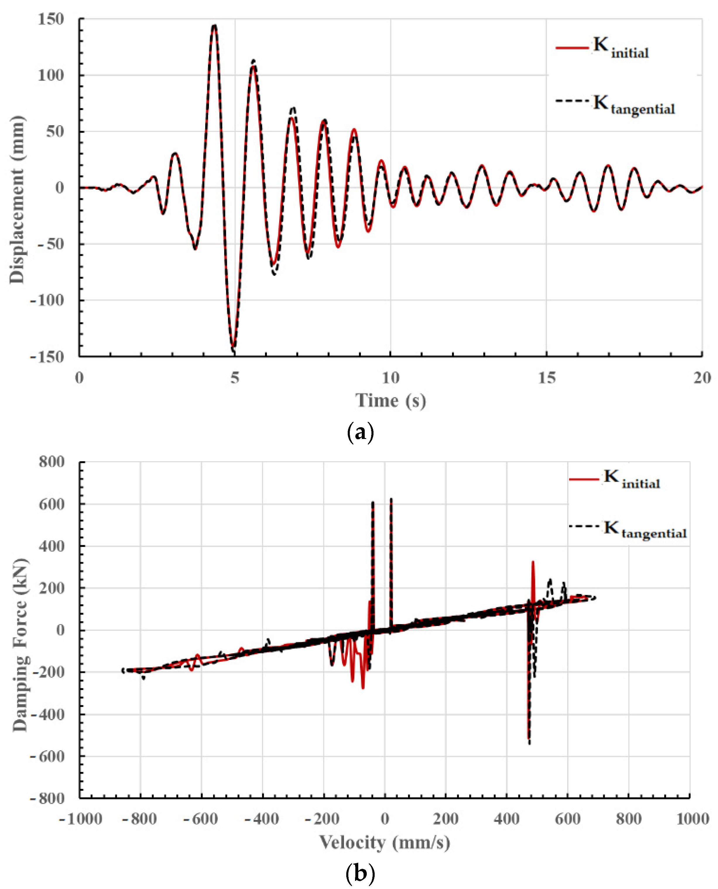
Step 3: Determine the total inelastic force ($F_N$) and tangent stiffness ‘$K_T$’ corresponds to the first mode elastic displacement calculated in Step 2 using the force–displacement backbone curve and the hysteresis model, presented in Section 2.2.

Step 4: For the first mode, determine the inelastic displacement, acceleration and velocity for the current time step using Equations (A1)–(A3) and Equation (A5) from Appendix A.

Step 5: Multiply the inelastic first mode responses (Step 4) and elastic higher mode responses (Step 2) with the modal coefficients (Step 1) to determine the MDOF modal responses. The time history response is determined by performing the direct sum (linear addition) of contributions from the individual modes of vibration. With modal analysis, the total maximum response is calculated using the SRSS combination method, which deals with peak responses corresponding to each significant mode of vibration occurring at different instances [22].

Step 6: Repeat Steps 2–5 for the full duration of each of the site-specific accelerograms. For each reference period group, calculate the design response by taking an arithmetic mean of the maximum responses.

The implementation of the above procedure is further demonstrated using a case study in Section 4.

2.1. Modal Analyses of the Stick Model

Dynamic modal properties: modal masses ‘$M_j$’, angular frequency (${\omega }_{n,j}$) and displacement coefficient ($P_j$) of the first three modes of vibration ‘j = 1 to j = 3’ can be determined either from eigen analysis (using computer software) or approximately calculated using empirical equations, given in [6]. For the first three modes of vibration, the value of ‘$M_j$’ can be approximated as 70%, 17% and 7% of the total mass of the building; ‘${\omega }_{n,j}$’ can be approximated as 1, 4 and 8 times of $\sqrt{K_{ini}/M_{j=1}}$; and the displacement coefficient at the roof level ‘$P_{j,roof}$’ may be taken as 1.43, 0.64 and 0.31, as recommended in [6,23,24] for a building having constant mass across the height and being supported by cantilever walls. The initial stiffness ‘$K_{ini}$’ (stiffness at or before the development of the first crack) is obtained from Section 2.2.

2.2. Inelastic Capacity and Hysteresis Modelling

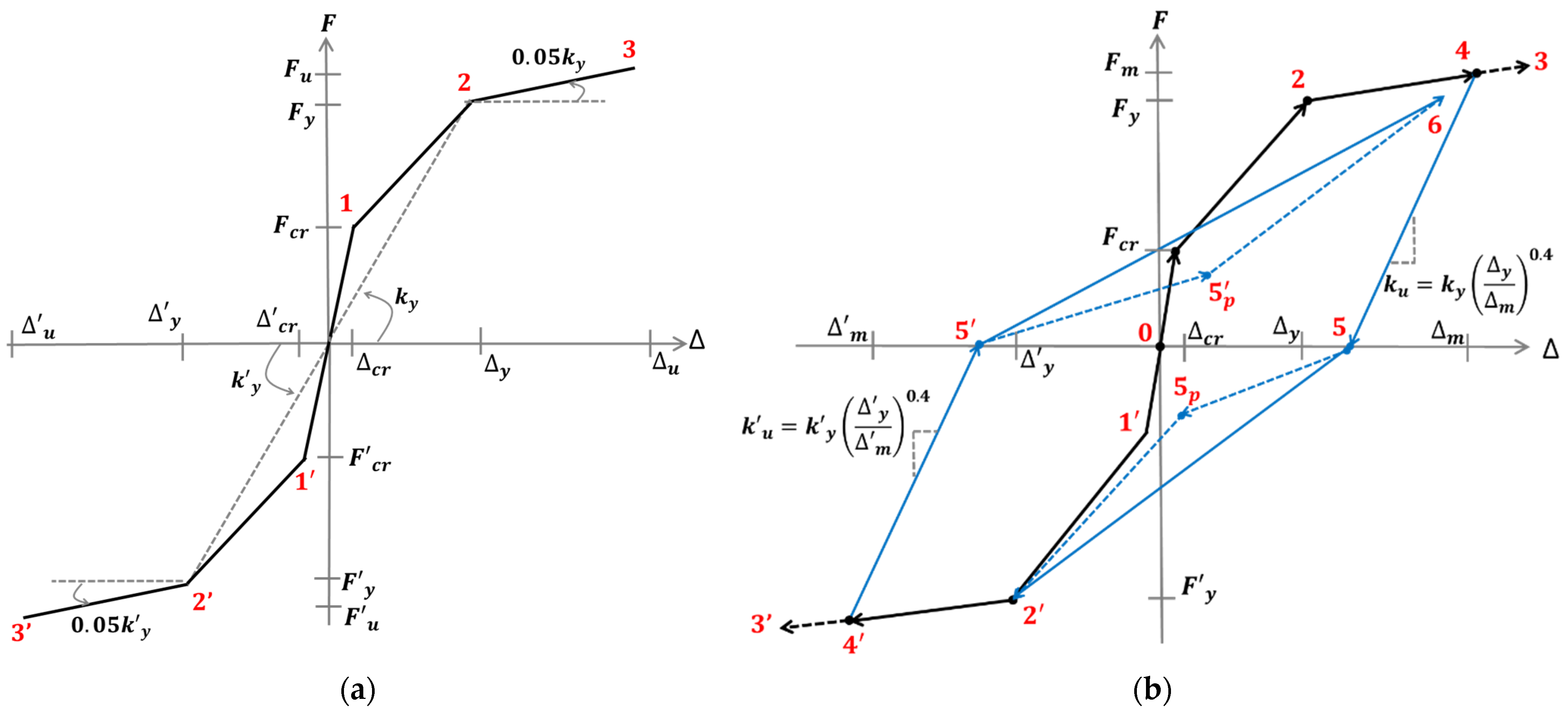
The inelastic capacity curve (referred herein as the pushover curve) that is used to model the nonlinear force–deformation behaviour of the plastic hinge is represented by the trilinear model at the system level (the whole building), as shown in Figure 3. The pushover curve at the system level is determined by superposing the force capacities of each structural element (structural walls or frames). Take the building shown in Figure 2 as an example. The capacity was derived by superposing the contributions of walls 1 and 2 whilst neglecting the out-of-plane contributions from walls 3 and 4. The simplified procedure, as outlined in Appendix B, is used to determine the force and displacement capacities of each structural element at the formation of the first crack (${∆}_{cr},F_{cr}$), the limit of the yield of the reinforcement (${∆}_y,F_y$) and the ultimate limit (${∆}_u,F_u$), where crushing of the concrete and crushing or buckling of the reinforcement occur, as represented, respectively, by points 1–3 (and 1′-3′ for reverse loading) of the trilinear backbone curve, as shown in Figure 3a. The input information required for the generation of the trilinear curve is the vertical reinforcement ratio and its diameter, the gross moment of area of the structural wall or column, the mean in situ strength of concrete, the yield strength and ultimate strength of the reinforcement, and the axial load ratio. More details of the simplified procedure can be found in Ref. [6].

The hysteresis model presented herein takes the trilinear form of the modified Takeda hysteresis rules [25]. The cyclic curves, which consider the effects of strain hardening, stiffness degradation, pinching and damages, as shown in Figure 3b, are achieved using the trilinear backbone curve, shown in Figure 3a. The backbone curve (from points 0 to 4) is used for the first cycle of loading. Upon unloading, unloading stiffness of ${k_u=k}_y{\left({∆}_y/{∆}_m\right)}^{0.4}$ is used first to reach zero force (point 5) and then it follows the backbone curve (points 2′ and 4′). On reloading, zero force (point 5′) is targeted prior to targeting the maximum deformation reached in the previous cycles (point 6 targeting at point 4). The alternative path with breakpoints 5_p and 5′_p is followed when pinching is of importance. In this study, the peak-oriented model as illustrated by the solid lines is adopted.

3. Operational Details with Applying NLTHA to MDOF Models

NLTHA on a full-scale MDOF model, or a finite element-based model, is considered to be the most direct and accurate method for capturing details of the dynamic response behaviour of the structure and its elements. Using NLTHA, the time history of the response for each degree of freedom can be simulated by solving the dynamic equation of equilibrium, as per Equation (1).

$$\left[M\right]\left\{\ddot{u}\left(t\right)\right\}+\left[C\right]\left\{\dot{u}\left(t\right)\right\}+f_s\left(\left\{u\left(t\right)\right\}\right)=-\left[M\right]\left\{1\right\}{\ddot{u}}_g\left(t\right)$$

(1)

where $\left[M\right] and \left[C\right]$ are $n\times n$ (n is the total number of degrees of freedom) matrices for defining the distribution of mass and damping behaviour of the structure, respectively; $f_s\left(\left\{u\left(t\right)\right\}\right)$ is the vector defining the lateral resistance developed in the structure expressed as a function of the lateral displacement of the DOFs; ${\ddot{u}}_g\left(t\right)$ is the earthquake acceleration time history that contains $m$ time steps; $\left\{\ddot{u}\left(t\right)\right\}$, and $\left\{\dot{u}\left(t\right)\right\}$ and $\left\{u\left(t\right)\right\}$ are $n\times m$ metrics that record the acceleration, velocity and displacement time histories of each degree of freedom throughout the event.

Due to the complexity involved in operating/dealing with matrices, such analysis is commonly performed using commercial packages such as SeismoStruct [14]. The underlying philosophy, including the details on how to derive entries to the matrices, is explained in Section 3.1, Section 3.2 and Section 3.3.

3.1. Mass Matrix

The mass matrix, $\left[M\right],$ is a diagonal matrix, with each entry representing a translational degree of freedom of the lumped mass. The seismic mass, computed as the imposed vertical load (including dead load and proportion of live load) divided by the gravitational acceleration $\prime g\prime$, is modelled as either lumped masses in the case of rigid diaphragms or distributed masses otherwise. The formation of the mass matrix [M] for the case of lumped masses is presented in Figure 4.

3.2. Force Matrix

The force vector, $f_s,$ can be used to calculate the tangential stiffness of the structural element at every time step following the hysteretic behaviour of the material whilst taking into account P-delta effects. The force vector is in turn derived from fibre element analysis in which the cross-section of a reinforced concrete element is subdivided into fibres of predefined stress–strain properties [14].

3.3. Damping Matrix

The damping matrix, $\left[C\right],$ models energy losses through dissipation mechanisms that cannot be explicitly accounted for by the hysteresis model. In NLTHA, significant energy dissipation is simulated by the hysteretic model to account for energy losses due to yielding or damage of the structural elements. The dissipated energy in each loading cycle is represented by the area within the loading path. The damping matrix covers any additional damping mechanisms (e.g., due to friction between the structure and the nonstructural elements, and nonlinear behaviour of the material prior to the occurrence of the first yield). The damping forces may be assumed to be viscous in nature, as represented by the damping term in Equation (1).

The practice of expressing the damping matrix as a linear function of the mass matrix and the stiffness matrix in the form as shown by Equation (2) has been established over a long time [26,27,28,29,30]. Targeting ${\zeta }_0$ at 5% equivalent viscous damping at both angular velocities is recommended, given that [20] suggests that time history analysis would usually adopt a damping value of 5%. This model of constructing the damping matrix is known as Rayleigh damping, which is most widely adopted by commercial software including ABAQUS [31] and SeismoStruct [14]. The main appeal is simplicity and computational efficiency. Mass proportional damping is a special form of Rayleigh damping, where β = 0 so that $\beta \left[K\right]$ is removed, leaving only the $\alpha \left[M\right]$ term. Likewise, stiffness proportional damping has only the $\beta \left[K\right]$ term. Alternatively, coefficients α and β can be calibrated to match the equivalent viscous damping ratio, ${\zeta }_0,$ to pre-determined values at two chosen angular velocities of vibration, ${\omega }_a$ and ${\omega }_b$, using Equations (3) and (4).

$$\left[C\right]=\alpha \left[M\right]+\beta \left[K\right]$$

(2)

$$\alpha =\frac{2{\omega }_a{\omega }_b{\zeta }_0}{{\omega }_a+{\omega }_b}$$

(3)

$$\beta =\frac{2{\zeta }_0}{{\omega }_a+{\omega }_b}$$

(4)

Input to the software is two data pairs: $({\omega }_a,{\zeta }_a)$ and $({\omega }_b,{\zeta }_b)$. In the example shown in Figure 5, the targeted value of $\zeta$ at the two natural frequencies was set at 5%. The two data pairs were accordingly $(10, 5\mathrm{\%})$ and $\left(200, 5\mathrm{\%}\right)$. Users of the model need to be wary of the implications of the shape of the curve, which is characteristic of Rayleigh damping. For example, very high modelled damping values outside the range bounded by the two angular frequencies mean that the affected modes of vibration can be very much suppressed. Thus, the data pairs (${\omega }_a, {\omega }_b$) must be carefully chosen. The New Zealand standards for earthquake actions, NZS 1170.5 [20], contain stipulations to control the choice of the data pairs. There can be significant spurious damping forces as the structure is excited into the inelastic range, resulting in the shifting of the natural frequencies, as discussed in [32,33].

Taking the $\left[K\right]$ matrix in Equation (2) as the tangential stiffness matrix, $\left[K_T\right],$ as opposed to the initial stiffness matrix, has the benefit of taking into account the effects of the reduction in the structural stiffness resulting from yielding. The modelling damping forces are accordingly lowered. The comparison between the initial stiffness matrix and tangential stiffness matrix within the Rayleigh framework is presented in Figure 6 in two formats: (a) displacement time histories, and (b) damping force versus velocity.

4. Case Study Analysis

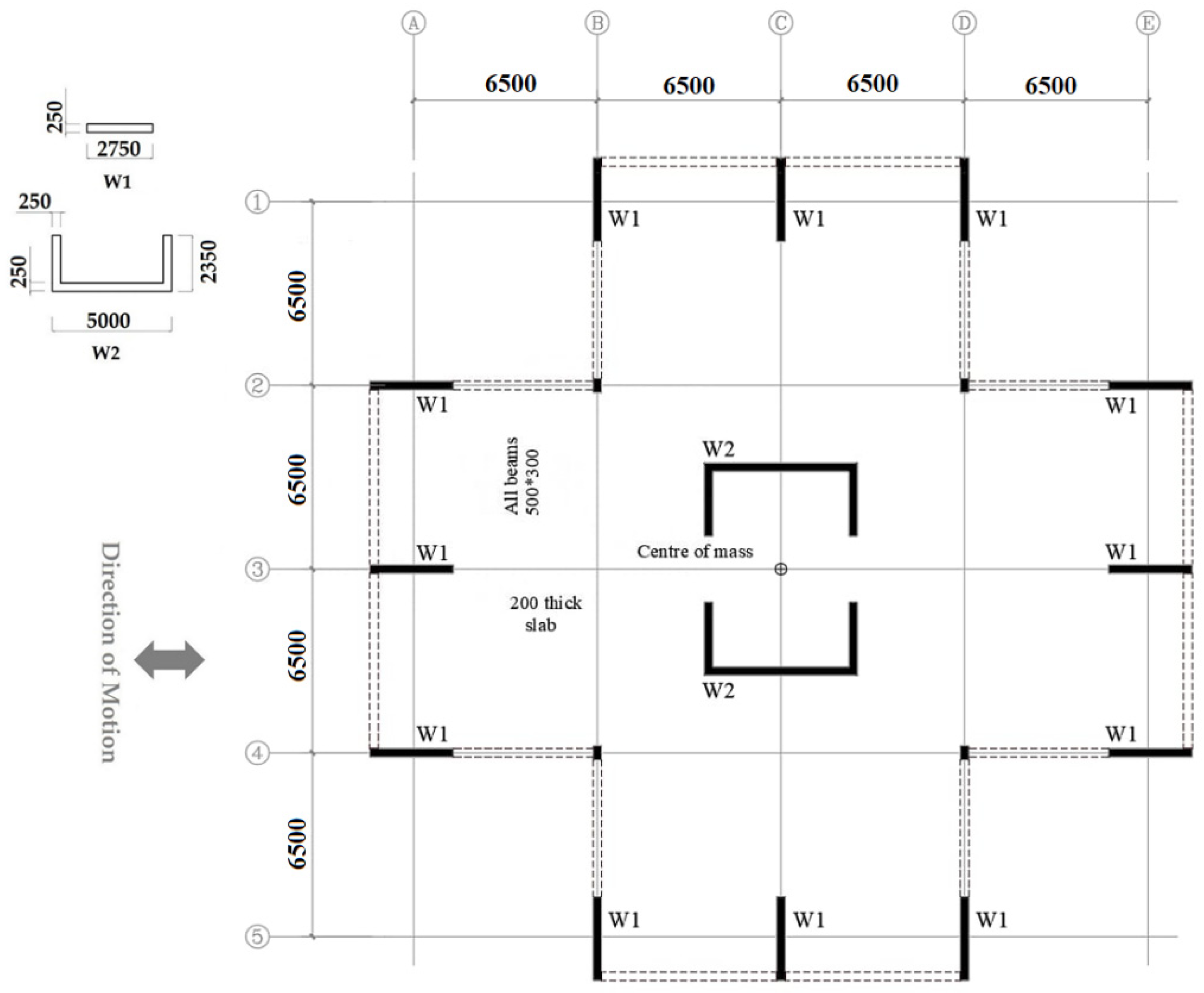
The application of the analytical procedure presented in this article is illustrated using a 10-storey case study building of 31 m in height, which has structural walls as the lateral load-resisting system. The floor plan and structural details of the building are shown in Figure 7. A building of this typical height and structural system is selected so that the first mode dominant structure and elastic higher mode responses assumed in RNLTHA are valid. The seismic lumped mass (dead load + 0.3 × imposed load) of 420 tonnes for each floor is calculated for an imposed load of 2 kPa, superimposed dead load of 1 kPa and façade load of 1 kPa. Material properties of the structural walls (W1 and W2) forming the seismic load-resisting system are presented in

Table 1. The material properties of RC walls of the case study building.

Parameters	Walls W1 and W2
$\mathrm{Diameter} \mathrm{of} \mathrm{vertical} \mathrm{reinforcement} \left(d_v\right)$	20 mm
$\mathrm{Vertical} \mathrm{reinforcement} \mathrm{ratio} \left(p_v\right)$	0.015 (1.5%)
$\mathrm{Yield} \mathrm{strength} \mathrm{of} \mathrm{reinforcement} {(f}_{sy})$	500 MPa
$\mathrm{Ultimate} \mathrm{strength} \mathrm{of} \mathrm{reinforcement} {(f}_{su})$	600 MPa
$\mathrm{Characteristic} \mathrm{strength} \mathrm{of} \mathrm{concrete} \left(f_c^{\mathrm{\prime }}\right)$	40 MPa
Axial load ratio (n)	0.11

. Results from dynamic modal analysis performed in SeismoStruct Version 2021 [14] are summarised in

Table 2. Dynamic properties of the case study building obtained from SeismoStruct [14].

Parameters	Mode 1	Mode 2	Mode 3
Modal mass (tonnes)	2735	840	290
Mass participation ratio (%)	65	20	7
Period (s)	0.82	0.15	0.05
$\mathrm{Displacement} \mathrm{coefficient} \mathrm{at} \mathrm{the} \mathrm{roof} \mathrm{level} ‘P_{j,roof}$’	1.56	0.70	0.33

. The first three modes of vibration have a combined effective modal mass participation of 92% of the total mass of the building.

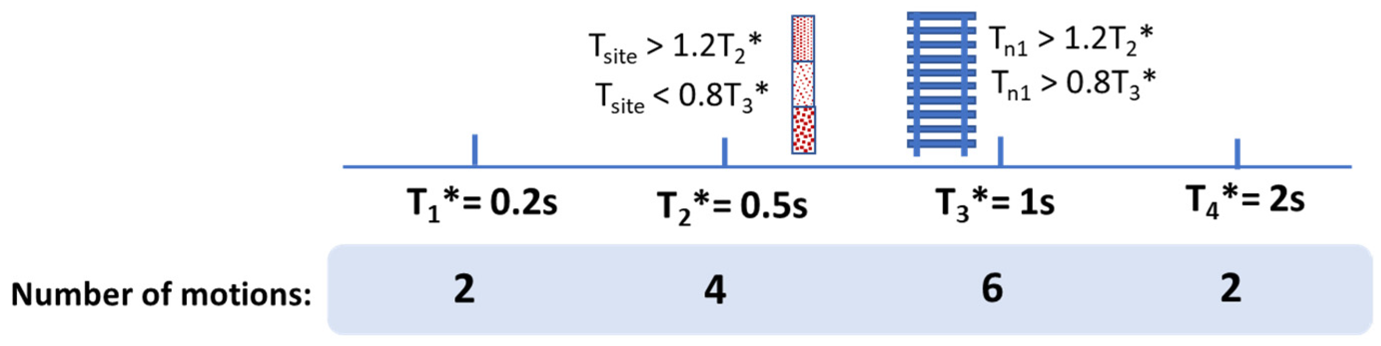
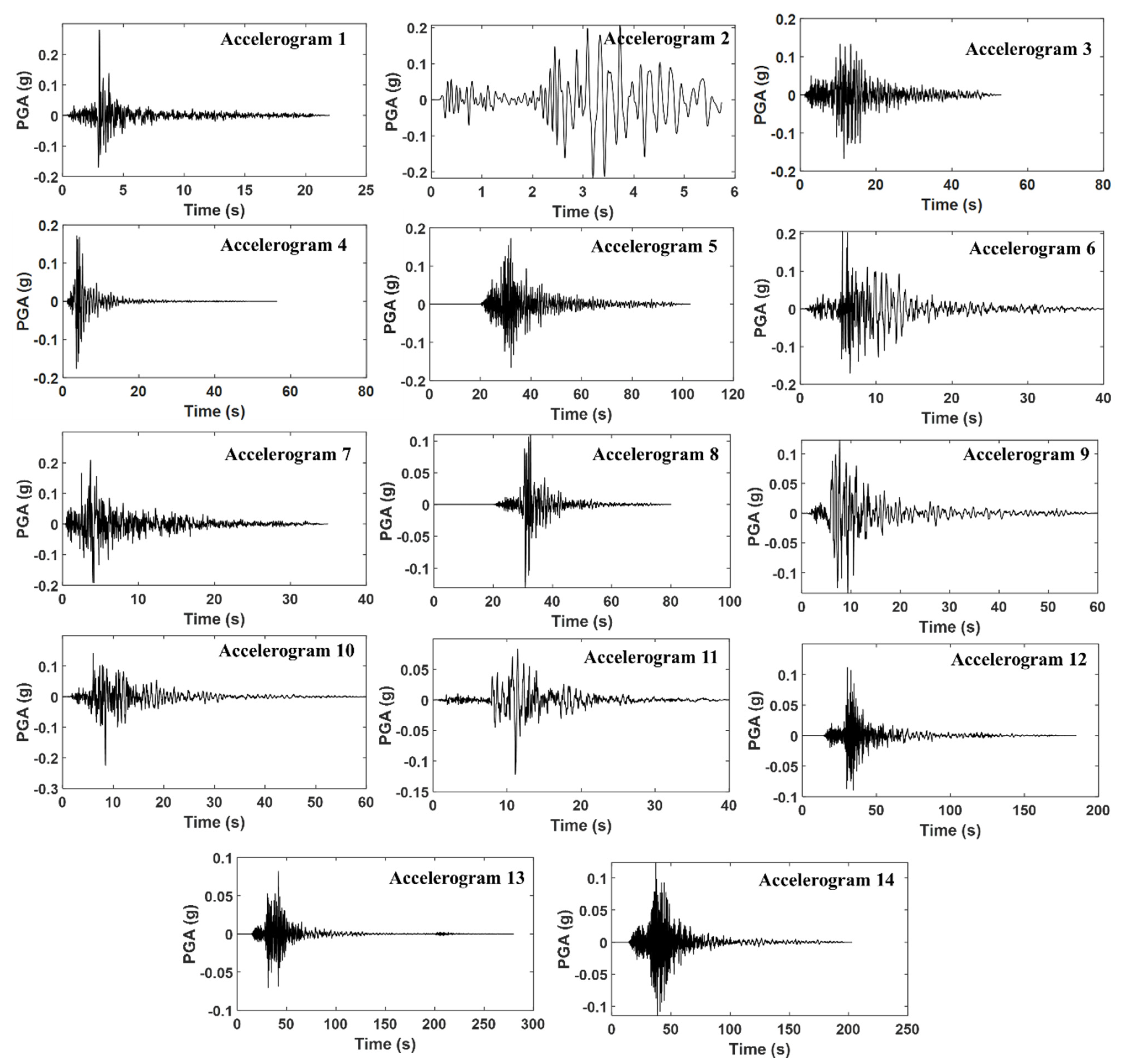
The design seismic hazard of 2% probability of exceedance in 50 years (2475 years return period earthquake), with a hazard value of 0.144 g, reverse/oblique fault, magnitude range of ±0.3 M_W, Joyner–Boore distance range of ±30 km and V_S,30 of 1000 m/s was specified when retrieving fourteen earthquake records from the PEER database. The selection scheme, which is presented diagrammatically in Figure 8 (showing the number of accelerograms for each reference period), was based on the recommendations in Ref. [10]. The listing of the selected earthquake records is presented in

Table A1. Summary of the earthquake records selected from the PEER database.

Ref. Period	Earthquake Name	Reference Periods (s)	Year	Station Name	Mw	Rjb (km)	PGA (g)	Scaling Factor
1	Whittier Narrows-02	0.2	1987	Mt Wilson—CIT Seis Sta	5.27	16.5	0.175	1.21
2	Northridge-06	0.2	1994	Beverly Hills—12520 Mulhol	5.28	10.6	0.130	0.85
3	Christchurch—2011	0.5	2011	GODS	5.79	9.1	0.175	0.63
4	Chi-Chi_ Taiwan-05	0.5	1999	HWA031	6.2	39.3	0.128	1.91
5	Chi-Chi_ Taiwan-05	0.5	1999	HWA005	6.2	32.7	0.124	1.46
6	Whittier Narrows-01	0.5	1987	Pacoima Kagel Canyon	5.99	31.6	0.169	1.04
7	Chi-Chi_ Taiwan-06	1	1999	CHY041	6.3	45.7	0.094	0.53
8	Chi-Chi_ Taiwan-06	1	1999	WHA019	6.3	52.4	0.087	1.68
9	Coalinga-01	1	1983	Parkfield—Fault Zone 11	6.36	27.1	0.084	1.08
10	Coalinga-01	1	1983	Parkfield—Stone Corral 3E	6.36	32.8	0.170	1.13
11	Northridge-01	1	1994	LA—Temple & Hope	6.69	28.8	0.113	0.62
12	San Fernando	1	1971	Lake Hughes #4	6.61	19.5	0.198	1.27
13	Loma Prieta	2	1989	SF—Diamond Heights	6.3	71.2	0.076	0.67
14	Iwate_ Japan	2	2008	Maekawa Miyagi Kawasaki City	6.9	74.8	0.159	0.95

in Appendix C. The bore log presented in Ref. [6] with a site period (T_site) of 0.61 s was subject to soil column site response analysis using the online tool available with free access at “quakeadvice.org” [11]. Fourteen soil surface accelerograms, as shown in Figure A1, were generated using the online tool.

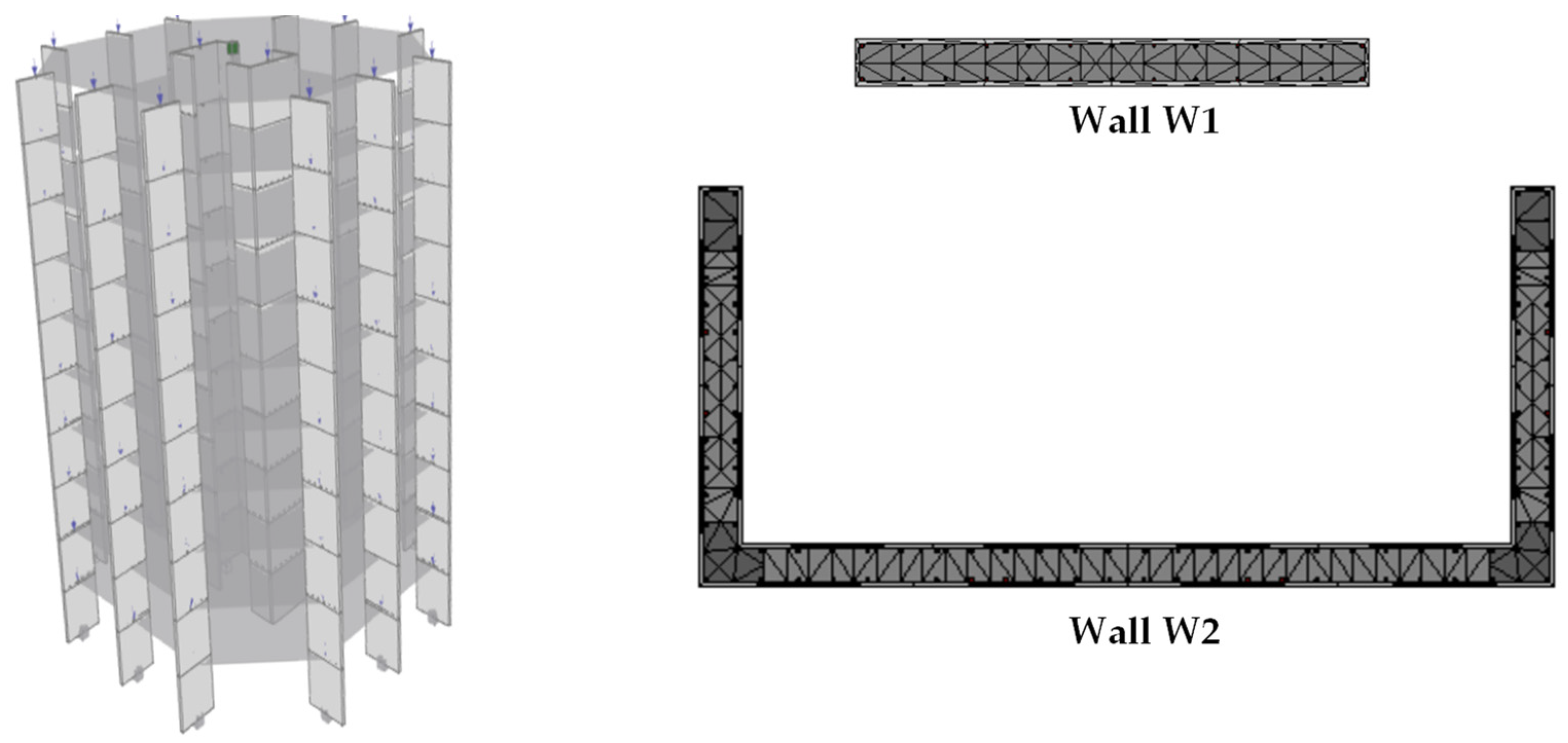
The proposed simplified nonlinear pushover analysis, as presented in Section 2.2, was used to construct the force–deformation curve of the building. The strength capacity of the building structure as a whole was calculated (at each of the displacement capacities) by superposing contributions from the six rectangular walls (W1) and two C-shaped walls (W2), whereas the displacement limit was controlled by the wall having the lowest yield displacement (wall W2). The calculations of the force and displacement capacities are shown below. The equations for the calculation of displacement and force capacities are given in Equations (A6)–(A11) and the input parameters required are given in

Table 3. Summary of the nonlinear parameters of the wall cross-sections.

Parameters	Wall W1	Wall W2
$H_e$	0.7 × 31 = 21.7 m	0.7 × 31 = 21.7 m
${\varphi }_{cr}$	2.10 × 10−4/mm	3.53 × 10−5/mm
${\varphi }_y$	0.0018/mm	5.48 × 10−4/mm
${\varphi }_u$	0.0081/mm	0.0045/mm
$E_c$	32,800 MPa	32,800 MPa
$I_{gross}$	4.33 × 1011 mm4	8.53 × 1012 mm4
$I_{eff}$	1.45 × 1011 mm4	2.86 × 1012 mm4
$L_p$	1363 mm	1588 mm
$L_{sp}$	220 mm	220 mm

. In Table 3, the curvatures ${\varphi }_{cr}$, ${\varphi }_y$ and ${\varphi }_u,$ the effective second moment of the section ($I_{eff}$) and the plastic hinge length ($L_p$) are determined using Equations (A12)–(A16) and information from Table 1.

Wall W1

At first crack: ${\Delta }_{cr}={\varphi }_{cr}{H}_e^2/3=33$ mm and $F_{cr}={\varphi }_{cr}{E}_c{I}_{gross}/H_e=139 \mathrm{kN}$

At yield point: ${\Delta }_y={\varphi }_y{H}_e^2/3=283$ mm and $F_y={\varphi }_y{E}_c{I}_{eff}/H_e=361 \mathrm{kN}$

At the ultimate point: ${∆}_u={\Delta }_y+\left({\varphi }_u-{\varphi }_y\right)L_p\times (H_e-0.5L_p+L_{sp})=466$ mm

$$\mathrm{and} F_u=F_y\left(1+0.05\left({∆}_u/{∆}_y-1\right)\right)=373 \mathrm{kN}$$

Wall W2

At first crack: ${\Delta }_{cr}={\varphi }_{cr}{H}_e^2/3=5.5$ mm and $F_{cr}={\varphi }_{cr}{E}_c{I}_{gross}/H_e=460\mathrm{kN}$

At yield point: ${\Delta }_y={\varphi }_y{H}_e^2/3=86$ mm and $F_y={\varphi }_y{E}_c{I}_{eff}/H_e=2162 \mathrm{kN}$

At the ultimate point: ${∆}_u={\Delta }_y+\left({\varphi }_u-{\varphi }_y\right)L_p\times (H_e-0.5L_p+L_{sp})=217$ mm

$$\mathrm{and} F_u=F_y\left(1+0.05\left({∆}_u/{∆}_y-1\right)\right)=2327 \mathrm{kN}$$

Combined or system level (corresponding forces at the level of displacement are determined using linear interpolation):

At first crack of ${\Delta }_{cr}=5.5$ mm, $F_{cr}=(139\times 5.5/33)\times 6+460\times 2=1059$ kN

At yield point of ${\Delta }_y=86$ mm, $F_y=186\times 6+2146\times 2=6458$ kN

At the ultimate point of ${∆}_u=217$ mm, $F_u=296\times 6+2327\times 2=6431$ kN

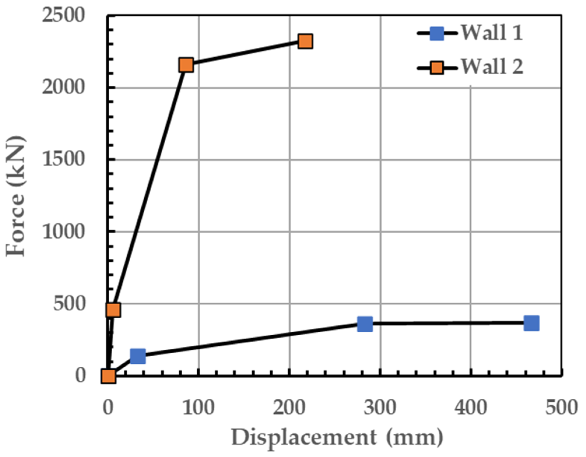
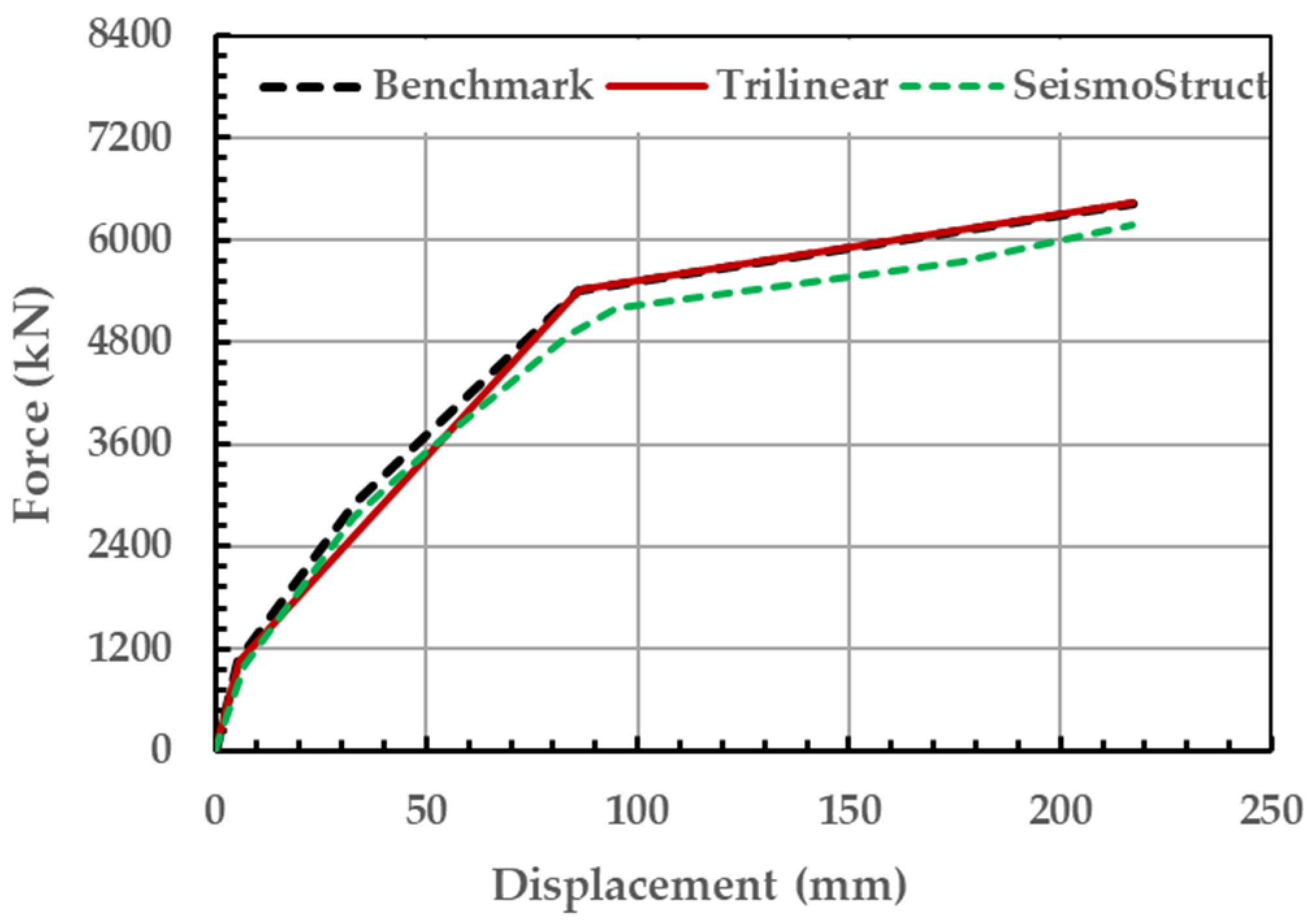
The trilinear force–displacement pushover curve obtained from the above calculations for wall W1 and wall W2 is presented in Figure 9. When the response from each wall is combined to determine the system pushover (i.e., using 6 × wall W1 and 2 × wall W2), referred to here as the ‘benchmark curve’, we no longer have a trilinear curve (refer to the black dashed line of Figure 10). This is because the cracking, yield and ultimate points for the respective walls do not have the same respective displacement values for each point. However, we can use engineering judgement to create a new trilinear curve to approximate the combined pushover response of the building (refer to the red line in Figure 10). Furthermore, the system-level pushover curve obtained from the pushover analysis of the building in SeismoStruct (refer to the green dashed line) was used to validate the simplified pushover curves. The comparison in Figure 10 shows that the simplified capacity curves (both benchmark and trilinear) introduced here are consistent with the curves obtained from SeismoStruct, which uses the fibre-based modelling approach [14].

The RNLTHA procedure of Section 2 (with a time step of 0.005 s) was employed to determine the time history response of the SDOF stick model. For validation and comparison purposes, the building was modelled, and nonlinear dynamic time history analysis was performed using SeismoStruct [14]. The building model in SeismoStruct consists of forced-based 3D frame elements featuring distributed inelasticity. The wall elements were interconnected at the floor levels by diaphragm actions. The cross-section of each wall was subdivided into fibres (each of which is 100 mm thick) across the depth and width of the wall cross-section, and five integration sections per storey, as shown in Figure 11, were used. The adopted material model is the cyclic uniaxial model of Mander et al. [34] for concrete and the Menegotto–Pinto model [35] for reinforcements. 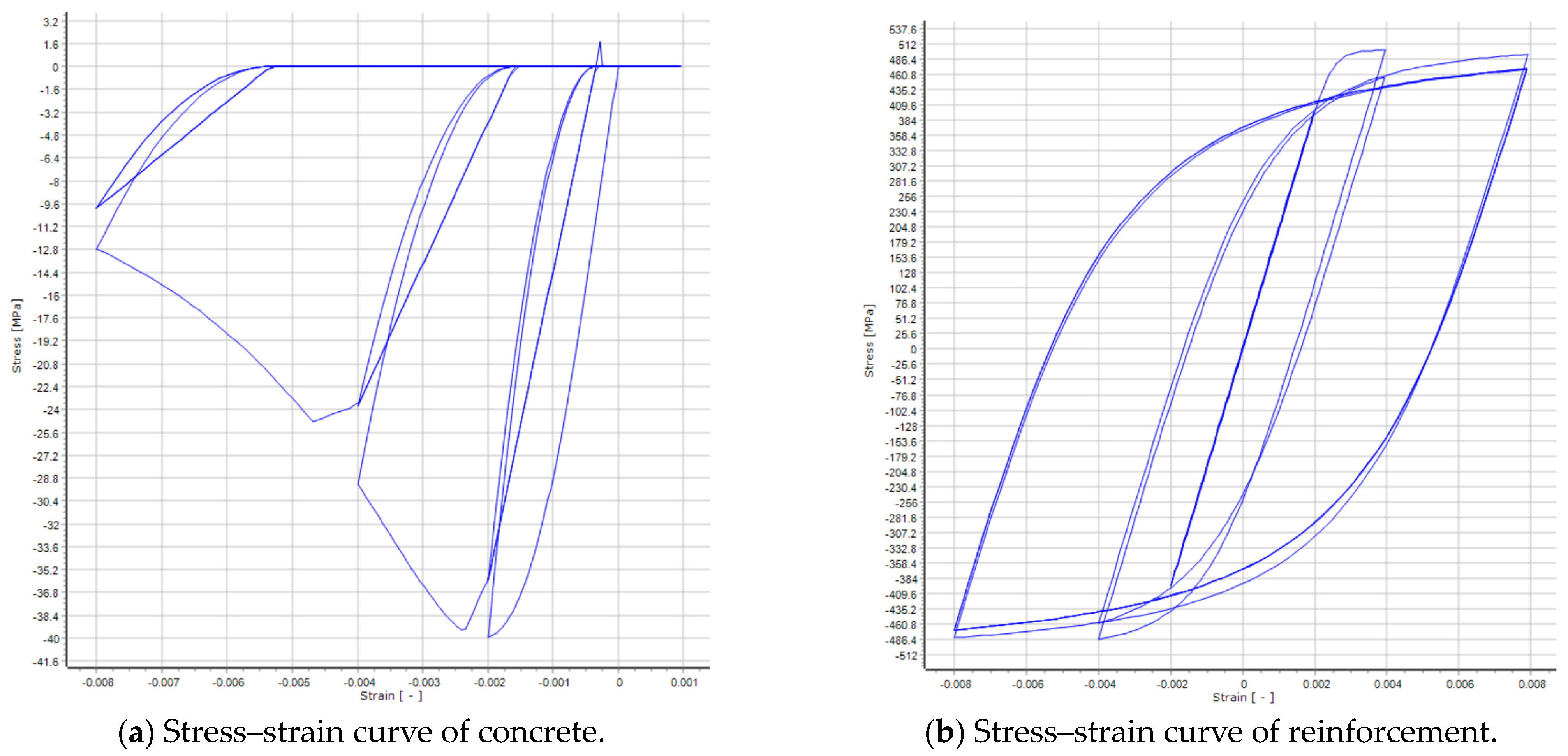The concrete and reinforcement strengths are listed in Table 2. Default values for strain hardening in steel and curve multipliers were adopted. The tensile strength of concrete is 2.5 MPa and the peak compressive strain is 0.0021. Material stress–strain curves used in the analyses can be found in Appendix D (Figure A2).

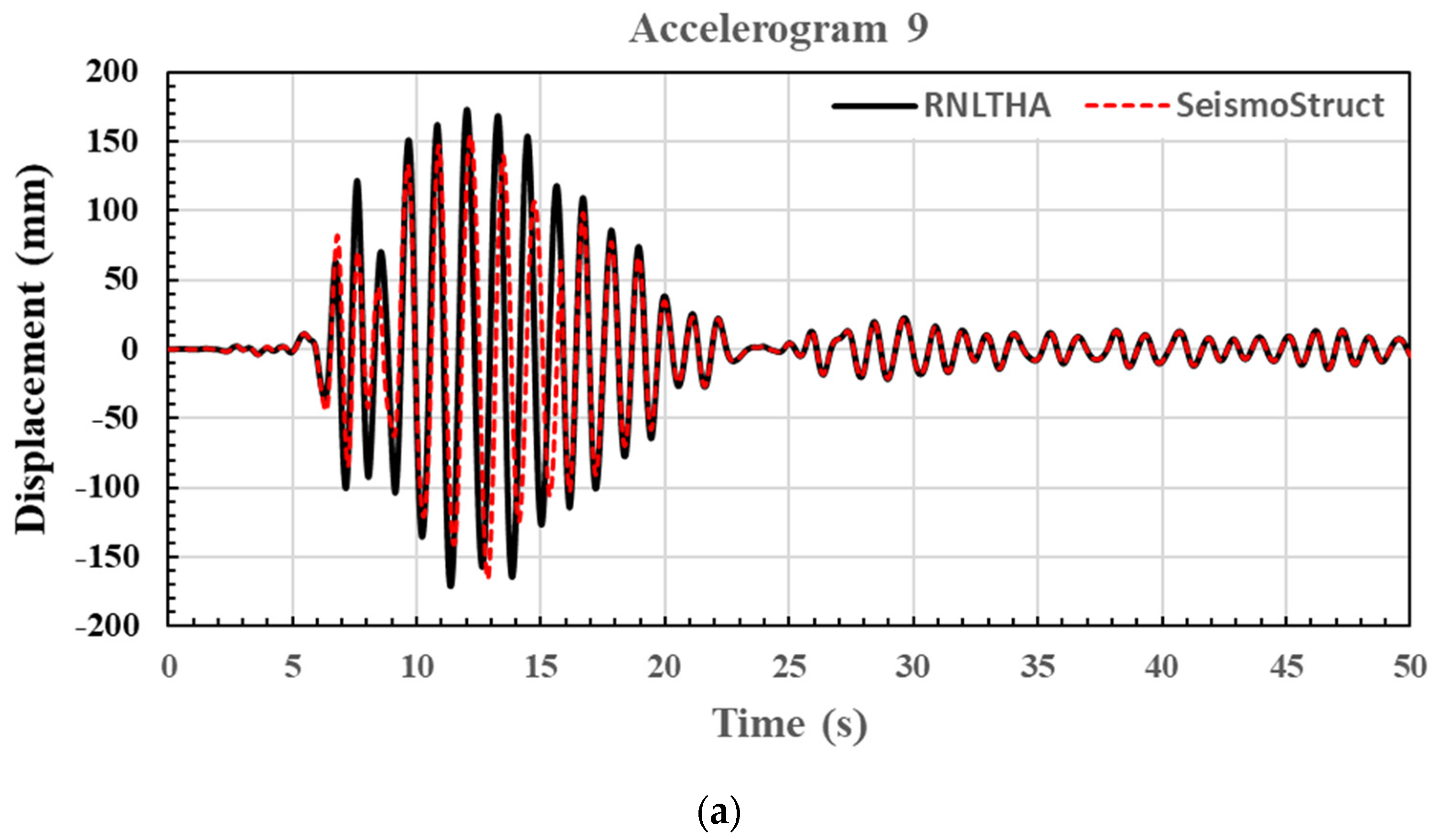
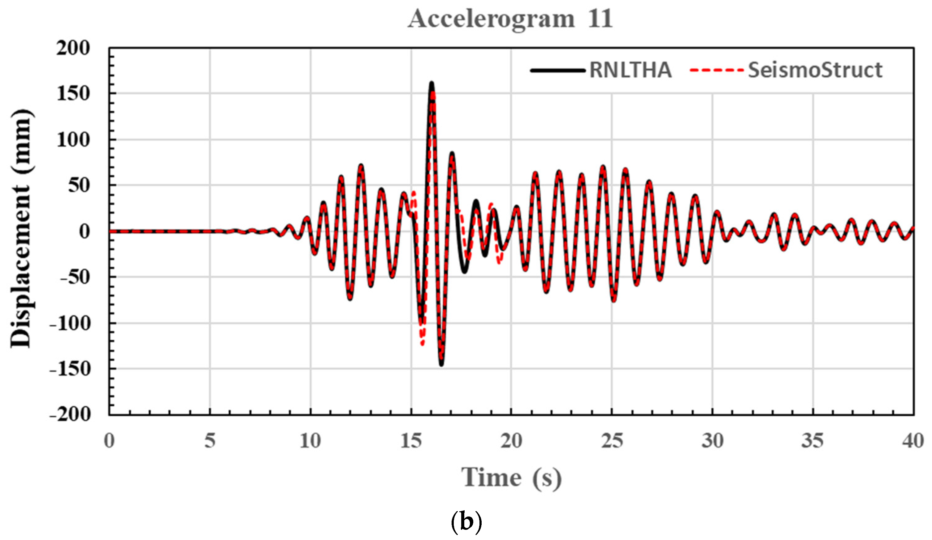
Comparisons of the displacement time history obtained from RNLTHA and SeismoStruct [14] are shown in Figure 12 for the soil surface accelerograms numbers 9 and 11, resulting in the highest peak displacement. Both accelerograms have a reference period (T*) of 1 s. From the comparison of displacement time history acquired from RNLTHA and SeismoStruct (Figure 12), it is shown that RNLTHA predicted the displacements in the elastic range (displacements < yield displacement of 86 mm) more accurately compared with the inelastic displacements (displacements > 86 mm). This is expected because the difference between the capacities predicted by the two methods increases in the inelastic range (refer to Figure 10). The treatment of the higher mode response as a purely elastic response may also have contributed to more discrepancies in the responses in the inelastic state.

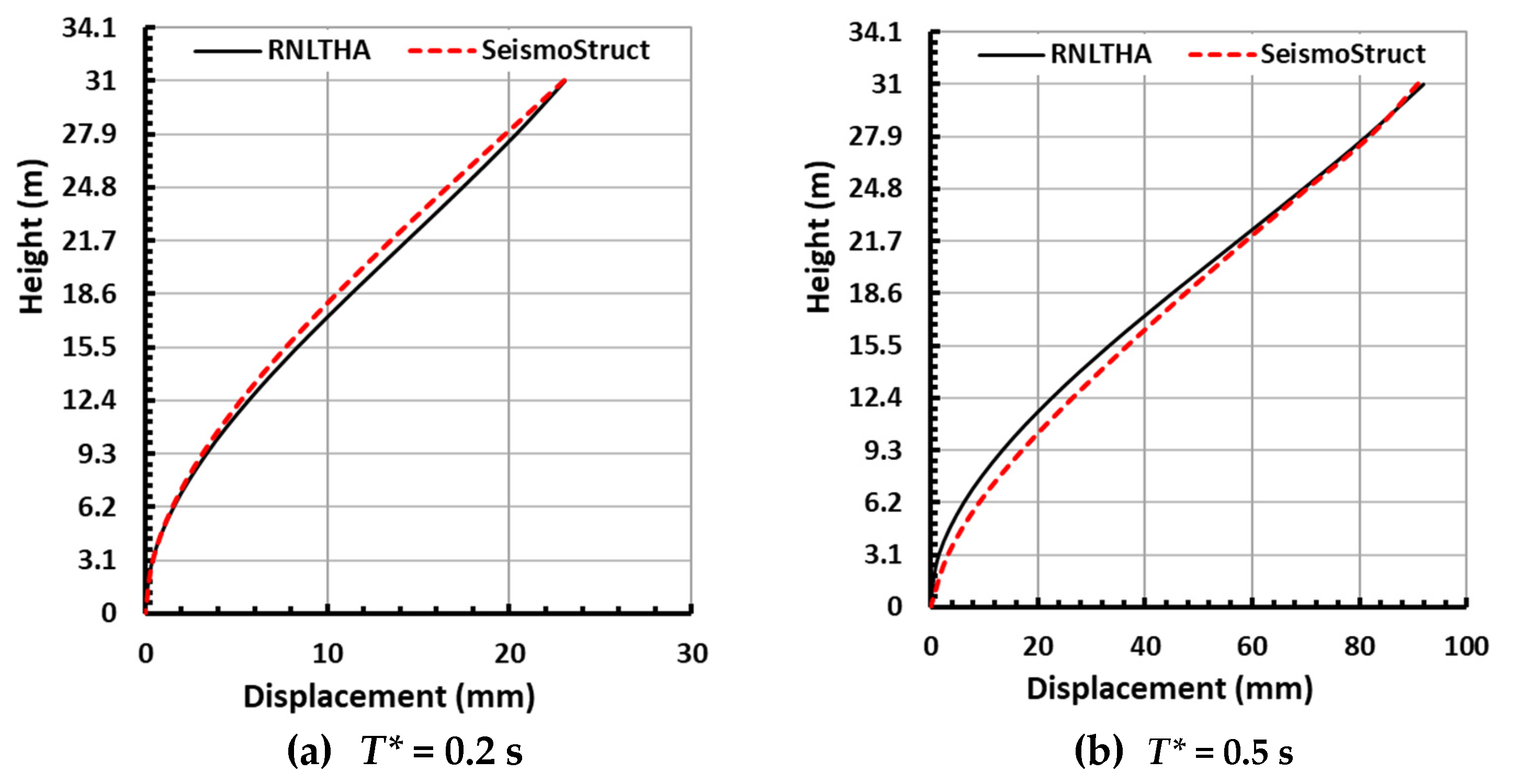
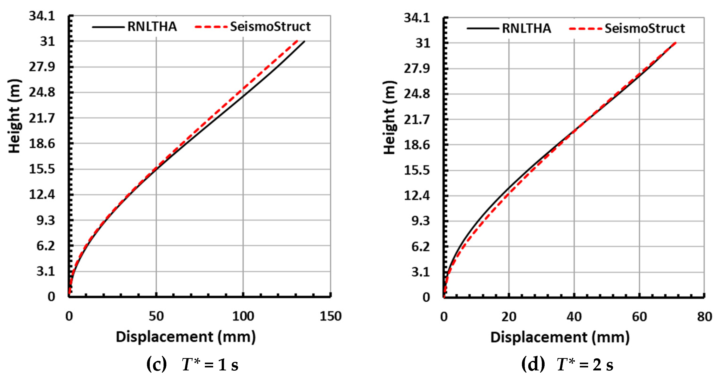
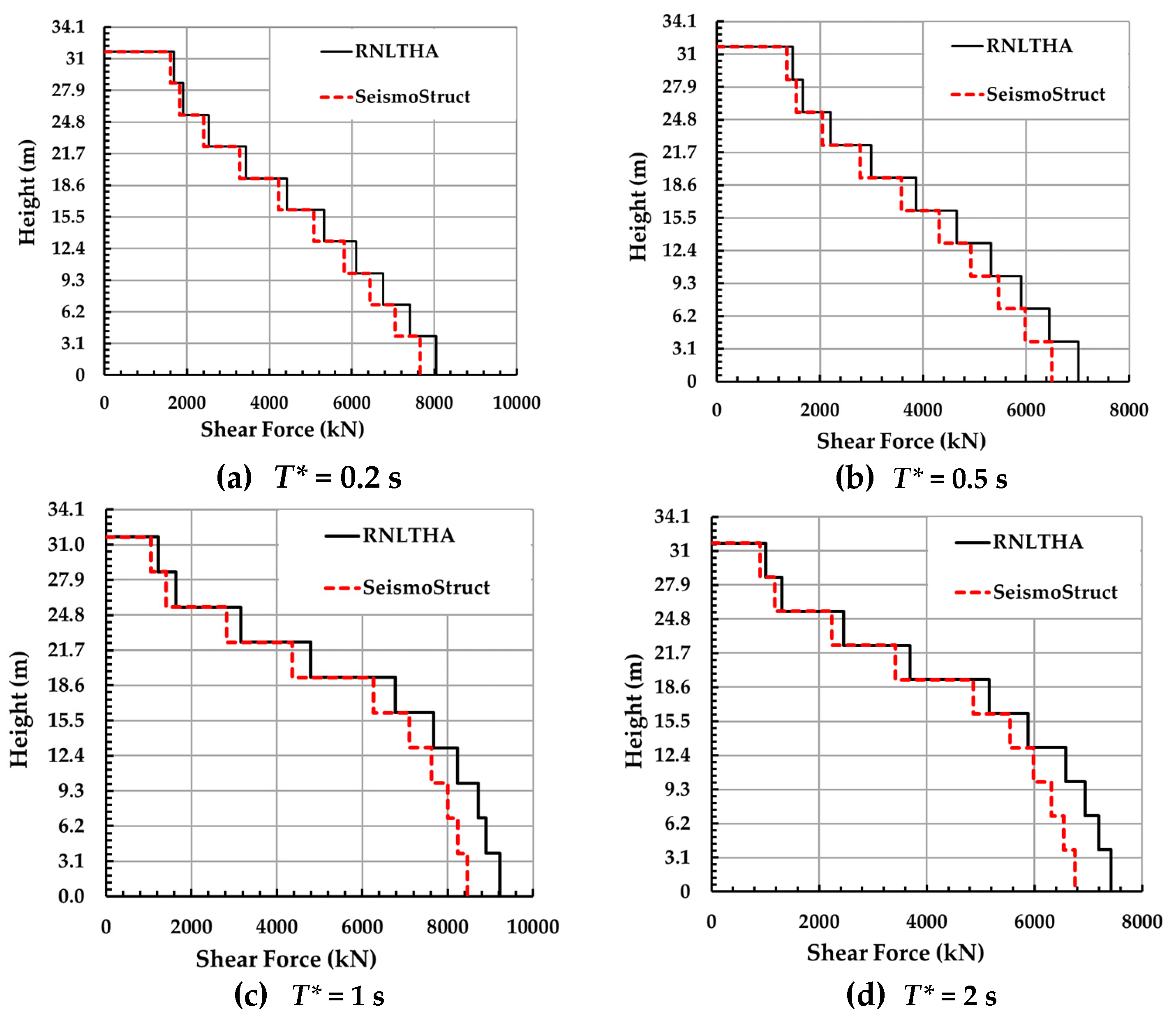
The displacement and storey shear profiles up the height of the building (for the case of the mean of the maximum response of each of the four reference periods) as obtained from the two methods are presented in Figure 13 and Figure 14, respectively. The difference between RNLTHA and SeismoStruct is within 10% for the roof displacement and base shear, and 20% for the storey shear. Given that RNLTHA reduces the computation time and costs by a significant amount, this difference is reasonable. The good agreement between the two sets of results for the case study building is mainly due to the facts that (1) the first mode of vibration dominates the response, (2) the lateral resistance of the building is contributed wholly by the structural walls, and (3) the response of the building as a whole is mainly within the elastic limit, except at the plastic hinges formed at the base of the structural walls.

The procedure proposed in this paper has been verified against commercial packages for a wall-type building model, where the gravity frame of the building is neglected. Depending on the structural configuration and sizing of elements, the gravity frame can affect the dynamic properties of the building and therefore cannot be neglected from the analysis model. The extension of RNLTHA to structures that are supported principally by frame actions or by a dual system of walls and frames is subjected to future study. Similarly, the trilinear pushover curve used in RNLTHA has been verified for buildings consisting of rectangular walls and walls of simple cross-sections, with a lower value of axial load ratio (typically less than 0.2). More case studies are to be investigated in future studies to check the suitability of the method in analysing buildings with complicated core walls, coupled walls and walls under the higher value of the axial load. Future research is also recommended for developing RNLTHA with a macroscopic model, with an MDOF system that can account more accurately for the compatibility forces that result from having slabs at all storeys.

5. Conclusions

This article presents the ‘rapid nonlinear time history analysis (RNLTHA)’ computational tool for producing robust predictions of the time history response of a reinforced concrete building responding to earthquake ground shaking. The analysis operates on a macro model, which takes the form of a stick with a lumped mass at the top and a hinge at the base to emulate the formation of a plastic hinge in concrete. A trilinear function is used to characterise the nonlinear properties of the base hinge. Nonlinear time history analysis is conducted through step-by-step integration. The analysis is best suited to dealing with a low-medium-rise building with structural walls (rectangular or/and simple cross-sections) as the lateral load-resisting system. The application of the method is illustrated with the case study of a ten-storey building. The procedure has a low computational memory demand, as the amount of computational time consumed is less than 5% of the analysis time of (general-purpose) finite element software like SeismoStruct. The generated results from RNLTHA and SeismoStruct were within 10% discrepancies for roof displacement and base shear, and a 20% difference for storey shear. Future research is suggested to extend the procedure for structures supported by frame actions or a combination of walls and frames, to include additional case studies to assess the method’s suitability for analysing buildings with complex core walls and coupled walls, and to develop the multi-degree-of-freedom system-based macroscopic model.

References

1. Wilson, E.L. Three Dimensional Static and Dynamic Analysis of Structures: A Physical Approach with Emphasis on Earthquake Engineering; Computers and Structures Incorporated: Walnut Creek, CA, USA, 1998. [Google Scholar]
2. Fajfar, P. A nonlinear analysis method for performance-based seismic design. Earthq. Spectra 2000, 16, 573–592. [Google Scholar] [CrossRef]
3. Chopra, A.K.; Goel, R.K. A modal pushover analysis procedure for estimating seismic demands for buildings. Earthq. Eng. Struct. Dyn. 2002, 31, 561–582. [Google Scholar] [CrossRef] [Green Version]
4. FEMA 356 FE. Prestandard and Commentary for the Seismic Rehabilitation of Buildings; Federal Emergency Management Agency: Washington, DC, USA, 2000.
5. Lagaros, N.D.; Mitropoulou, C.C.; Papadrakakis, M. Time history seismic analysis. In Encyclopedia of Earthquake Engineering; Spinger: Berlin/Heidelberg, Germany, 2013; pp. 1–19. [Google Scholar] [CrossRef]
6. Khatiwada, P.; Hu, Y.; Lumantarna, E.; Menegon, S.J. Dynamic Modal Analyses of Building Structures Employing Site Specific Response Spectra Versus Code Response Spectrum Models. CivilEng 2023, 4, 134–150. [Google Scholar] [CrossRef]
7. Hu, Y.; Lam, N.; Menegon, S.J.; Wilson, J.L. The Selection and Scaling of Ground Motion Accelerograms for Use in Stable Continental Regions. J. Earthq. Eng. 2022, 26, 6284–6303. [Google Scholar] [CrossRef]
8. Hu, Y.; Lam, N.; Khatiwada, P.; Menegon, S.J.; Looi, D.T.W. Site-specific response spectra: Guidelines for engineering practice. CivilEng 2021, 2, 712–735. [Google Scholar] [CrossRef]
9. Khatiwada, P.; Hu, Y.; Lam, N.; Lumantarna, E. Program on Generation of Site-Specific Response Spectra in Australia. In Proceedings of the Australian Earthquake Engineering Society 2021, Online, 25–26 November 2021. [Google Scholar]
10. Hu, Y.; Lam, N.; Khatiwada, P.; Lumantarna, E.; Tsang, H.H.; Menegon, S.J. Site-specific response spectra and accelerograms on bedrock and soil surface. CivilEng 2023, 4, 311–332. [Google Scholar] [CrossRef]
11. QuakeAdvice. Site Specific Response Spectrum. Available online: http://quakeadvice.org/index.php/advanced-seismic-design/australia-adv/site-specific-response-spectrum/ (accessed on 10 December 2022).
12. Datta, T.K. Seismic Analysis of Structures; John Wiley & Sons: Hoboken, NJ, USA, 2010. [Google Scholar]
13. The MathWorks Inc. MATLAB Version: 9.13.0 (R2022b). Available online: https://www.mathworks.com (accessed on 7 July 2023).
14. SeismoStruct—A Computer Program for Static and Dynamic Nonlinear Analysis of Framed Structures. Available online: www.seismosoft.com (accessed on 10 December 2022).
15. Priestly, M.J.N.; Calvi, G.M.; Kowalsky, M.J. Displacement-Based Seismic Design of Structures; IUSS PRESS: Pavia, Italy, 2007. [Google Scholar]
16. Priestley, M.J.N. Does capacity design do the job? An examination of higher mode effects in cantilever walls. Bull. N. Z. Soc. Earthq. Eng. 2003, 36, 276–292. [Google Scholar] [CrossRef] [Green Version]
17. Priestley, M.J.N.; Amaris, A.D. Dynamic amplification of seismic moments and shears in cantilever walls. In European School for Advanced Studies in Reduction of Seismic Risk; Union of International Associations: Brussels, Belgium, 2002. [Google Scholar]
18. Sullivan, T.J.; Priestley, M.J.N.; Calvi, G.M. Estimating the higher-mode response of ductile structures. J. Earthq. Eng. 2008, 12, 456–472. [Google Scholar] [CrossRef]
19. Hu, Y.; Khatiwada, P.; Lumantarna, E.; Lam, N.; Tsang, H.H. Assessment of torsional amplification of drift demand in buildings employing site specific response spectra and accelerograms. CivilEng 2023, 4, 248–269. [Google Scholar] [CrossRef]
20. Menegon, S.J.; Wilson, J.L.; Lam, N.T.K. (Eds.) AS 1170.4-2007 Structural design actions Part 4: Earthquake actions in Australia, 2nd Edition. In Proceedings of the AEES Conference, Online, 25–26 November 2021; University of Queensland: Queensland, Australia, 2021. [Google Scholar]
21. NZS 1170.5; 2004 Structural Design Actions Part 5: Earthquake Actions. Standards New Zealand: Wellington, New Zealand, 2004.
22. Mehmood, T.; Warnitchai, P.; Suwansaya, P. Seismic evaluation of tall buildings using a simplified but accurate analysis procedure. J. Earthq. Eng. 2018, 22, 356–381. [Google Scholar] [CrossRef]
23. Lumantarna, E.; Mehdipanah, A.; Lam, N.; Wilson, J. Methods of structural analysis of buildings in regions of low to moderate seismicity. In Proceedings of the 2017 World Congress on Advances in Structural Engineering and Mechanics (ASEM17), Seoul, Republic of Korea, 28 August–1 September 2017. [Google Scholar]
24. Fardipour, M.; Lumantarna, E.; Lam, N.; Wilson, J.; Gad, E. Drift demand predictions in low to moderate seismicity regions. Aust. J. Struct. Eng. 2010, 11, 195–206. [Google Scholar] [CrossRef]
25. Takeda, T.; Sozen, M.A.; Nielsen, N.N. Reinforced concrete response to simulated earthquakes. J. Struct. Div. 1970, 96, 2557–2573. [Google Scholar] [CrossRef]
26. Rayleigh, J.W.S.B. The Theory of Sound; Macmillan & Company: London, UK, 1896; Volume 2. [Google Scholar]
27. Adhikari, S. Damping modelling using generalized proportional damping. J. Sound Vib. 2006, 293, 156–170. [Google Scholar] [CrossRef]
28. Chopra, A.K.; McKenna, F. Modeling viscous damping in nonlinear response history analysis of buildings for earthquake excitation. Earthq. Eng. Struct. Dyn. 2016, 45, 193–211. [Google Scholar] [CrossRef]
29. Lee, C.L. Proportional viscous damping model for matching damping ratios. Eng. Struct. 2020, 207, 110178. [Google Scholar] [CrossRef]
30. Liu, M.; Gorman, D.G. Formulation of Rayleigh damping and its extensions. Comput. Struct. 1995, 57, 277–285. [Google Scholar] [CrossRef]
31. Smith, M. ABAQUS/Standard User’s Manual; Version 6.9; ABAQUS: Washington, DC, USA, 2009. [Google Scholar]
32. Bernal, D. Viscous damping in inelastic structural response. J. Struct. Eng. 1994, 120, 1240–1254. [Google Scholar] [CrossRef]
33. Hall, J.F. Problems encountered from the use (or misuse) of Rayleigh damping. Earthq. Eng. Struct. Dyn. 2006, 35, 525–545. [Google Scholar] [CrossRef]
34. Mander, J.B.; Priestley, M.J.; Park, R. Theoretical stress-strain model for confined concrete. J. Struct. Eng. 1988, 114, 1804–1826. [Google Scholar] [CrossRef] [Green Version]
35. Menegotto, M.; Pinto, P.E. Method of analysis for cyclically loaded R.C. plane frames including changes in geometry and non-elastic behaviour of elements under combined normal force and bending. In Proceedings of the Symposium on the Resistance and Ultimate Deformability of Structures Acted on by Well Defined Repeated Loads; International Association for Bridge and Structural Engineering: Zurich, Switzerland, 1973; pp. 15–22. [Google Scholar]
36. Newmark, N.M. A method of computation for structural dynamics. J. Eng. Mech. Div. 1959, 85, 67–94. [Google Scholar] [CrossRef]
Figure 1. Comparison of the number of degrees of freedom to be solved in the proposed 2D finite element-based model and the counterpart macroscopic model. (a) Finite element model of a shear wall (≈2100 DOFs). (b) Macroscopic model (2 DOFs).
Civileng 04 00048 g001
Figure 2. The macroscopic model used in RNLTHA. The multi-storey building model at the top is transformed into the three stick models at the bottom, which have in total 4 DOFs, represented by numbers 1–4 in green. The nonlinearity is considered through the plastic hinge rotation for the first mode only.
Civileng 04 00048 g002
Figure 3. Modelling of the material nonlinearity and hysteresis in the simplified procedure. (a) Trilinear pushover backbone curve. (b) Hysteresis modelling rules.
Civileng 04 00048 g003
Figure 4. Mass matrix of the MDOF lumped mass system.
Civileng 04 00048 g004
Figure 5. Damping curve from the Rayleigh damping model anchoring at two data pairs: (10, 5%) and (200, 5%).
Civileng 04 00048 g005
Figure 6. Comparison of the displacement time history and velocity vs. damping force history obtained using initial and tangential stiffness-based Rayleigh damping. (a) Time history of displacement response. (b) Velocity vs. damping force during the excitation.
Civileng 04 00048 g006
Figure 7. Details of the case study building showing the floor plan and structural layout.
Civileng 04 00048 g007
Figure 8. Accelerogram selection scheme for the case study building (Tsite = 0.61 s and Tn1 = 0.82 s).
Civileng 04 00048 g008
Figure 9. Simplified trilinear pushover capacity curves obtained for walls W1 and W2 of the case study building.
Civileng 04 00048 g009
Figure 10. Capacity curves of the case study building obtained from the simplified method and SeismoStruct [14]. The red line representing the trilinear curve is used in RNLTHA.
Civileng 04 00048 g010
Figure 11. SeismoStruct model of the case study building showing element connectivity and the detail of the element discretization.
Civileng 04 00048 g011
Figure 12. Displacement response time history at the roof level of the case study building when subject to the two most critical soil surface accelerograms with a reference period of 1 s. (a) Accelerogram 9. (b) Accelerogram 11.
Civileng 04 00048 g012aCivileng 04 00048 g012b
Figure 13. Mean of the maximum storey displacement profile obtained from RNLTHA and SeismoStruct for each of the four reference periods (T*).
Civileng 04 00048 g013aCivileng 04 00048 g013b
Figure 14. Mean of the maximum storey shear profile obtained from RNLTHA and SeismoStruct for each of the four reference periods (T*).
Civileng 04 00048 g014