
Assessing Landslide Susceptibility in the Northern Stretch of Arun Tectonic Window, Nepal


Abstract
:1. Introduction
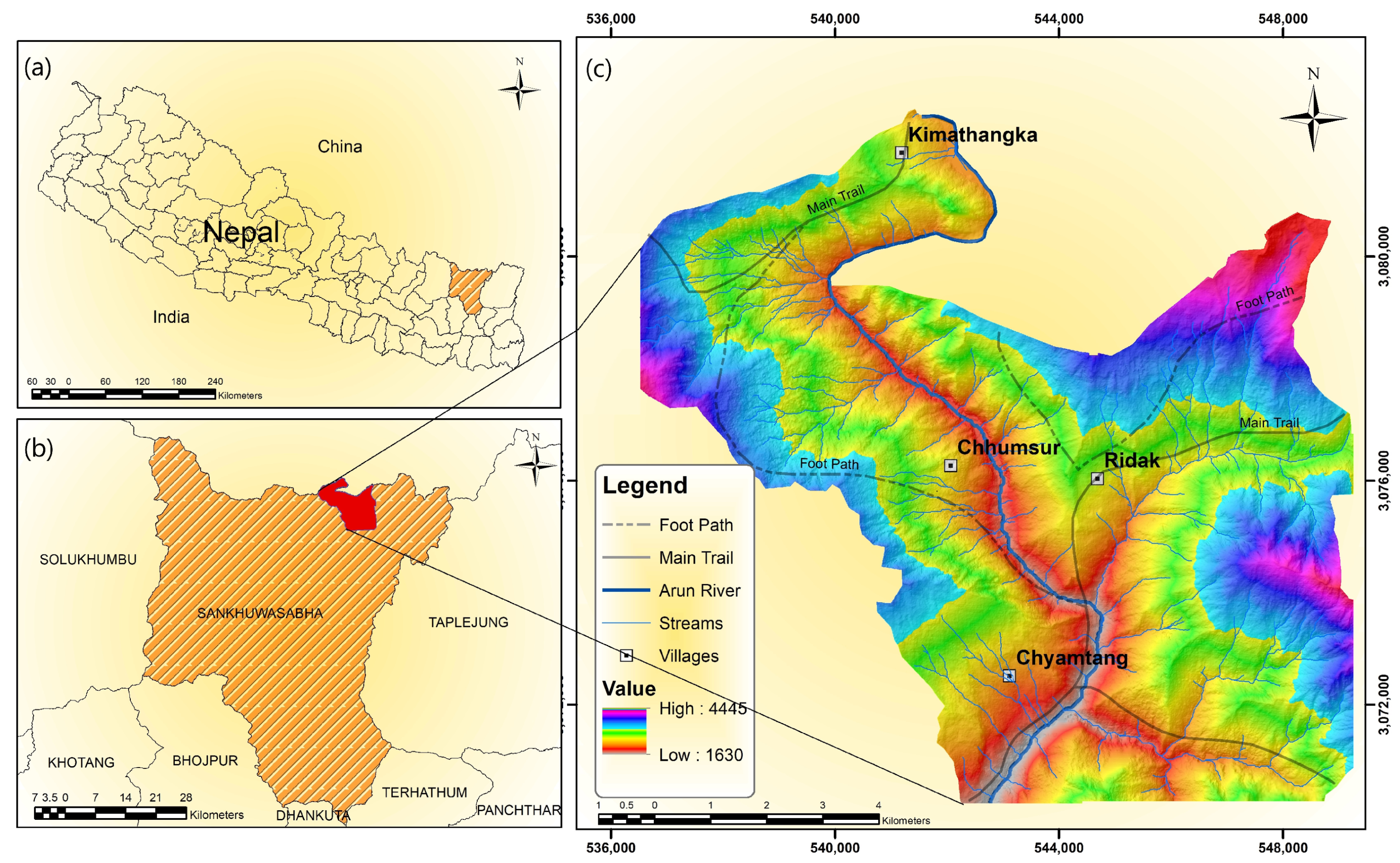
2. Study Area


3. Method
3.1. Data Acquisition and Processing

3.2. Landslide Susceptibility Modeling
Weight of Evidence Method
3.3. Frequency Ratio Method
4. Results
4.1. Influencing Factors
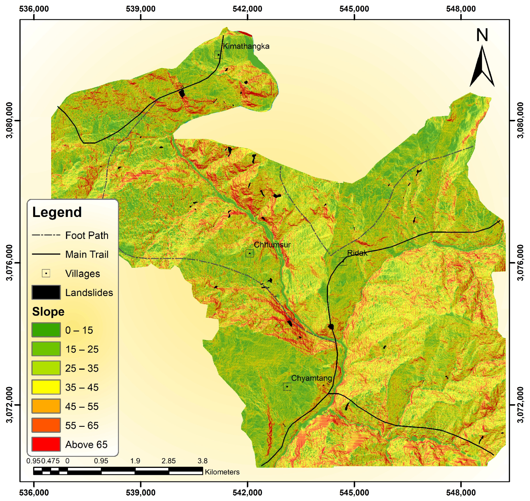
4.1.1. Slope Angle
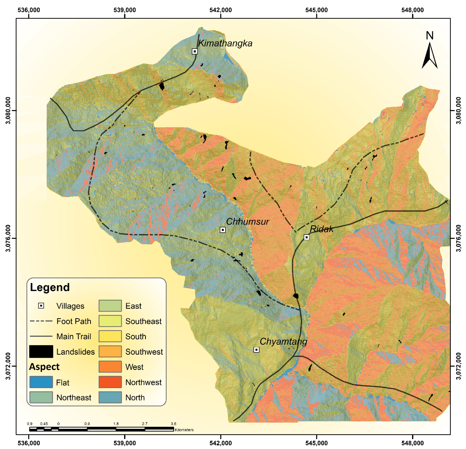
4.1.2. Slope Aspect
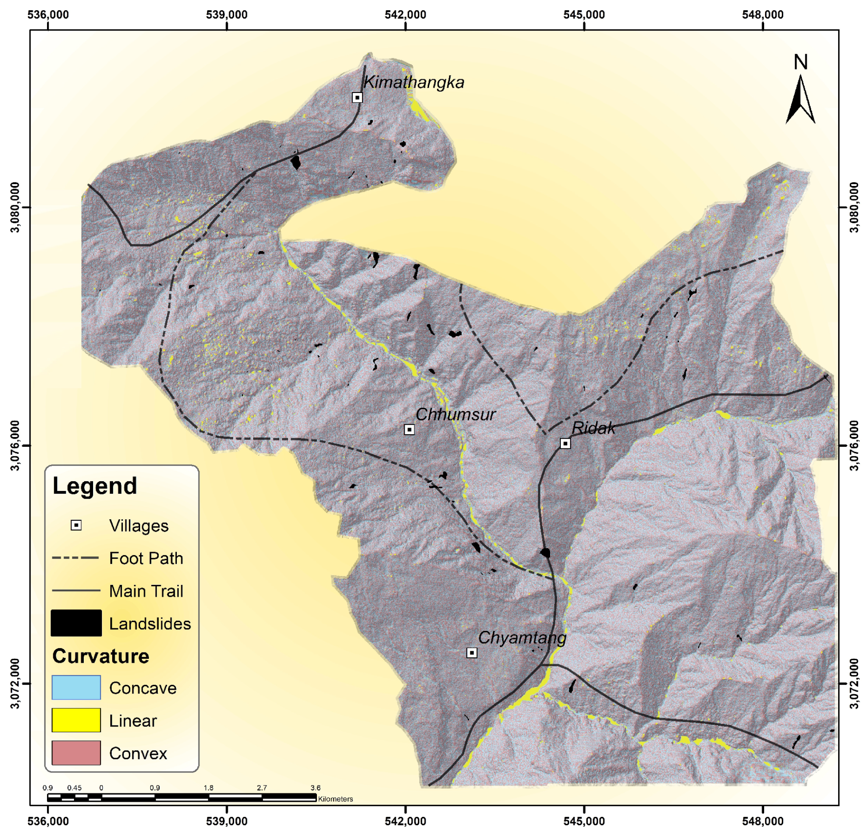
4.1.3. Slope Shape
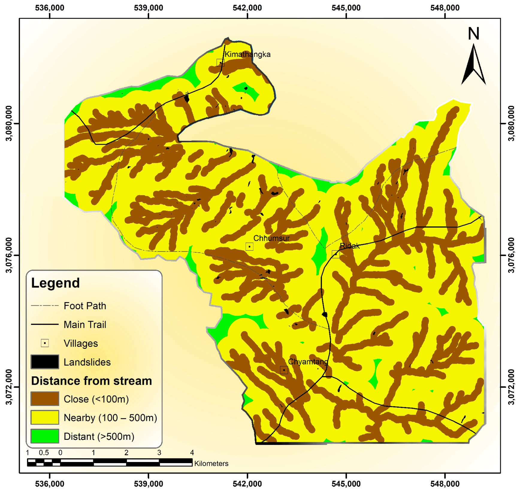
4.1.4. Stream Proximity
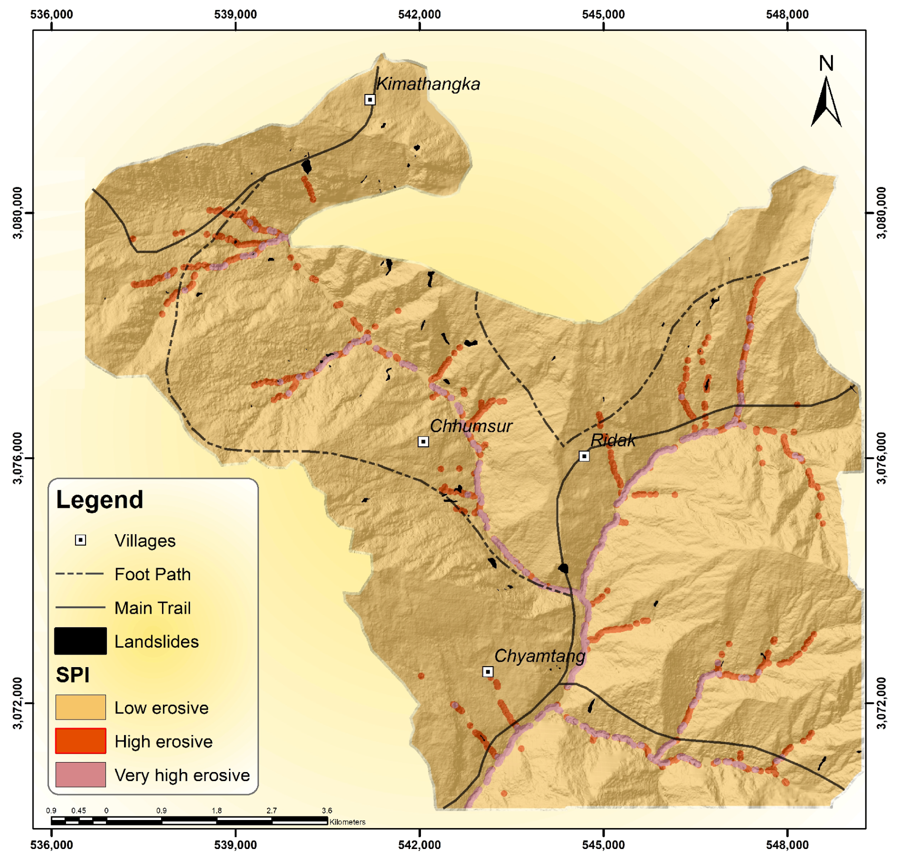
4.1.5. Stream Power Index
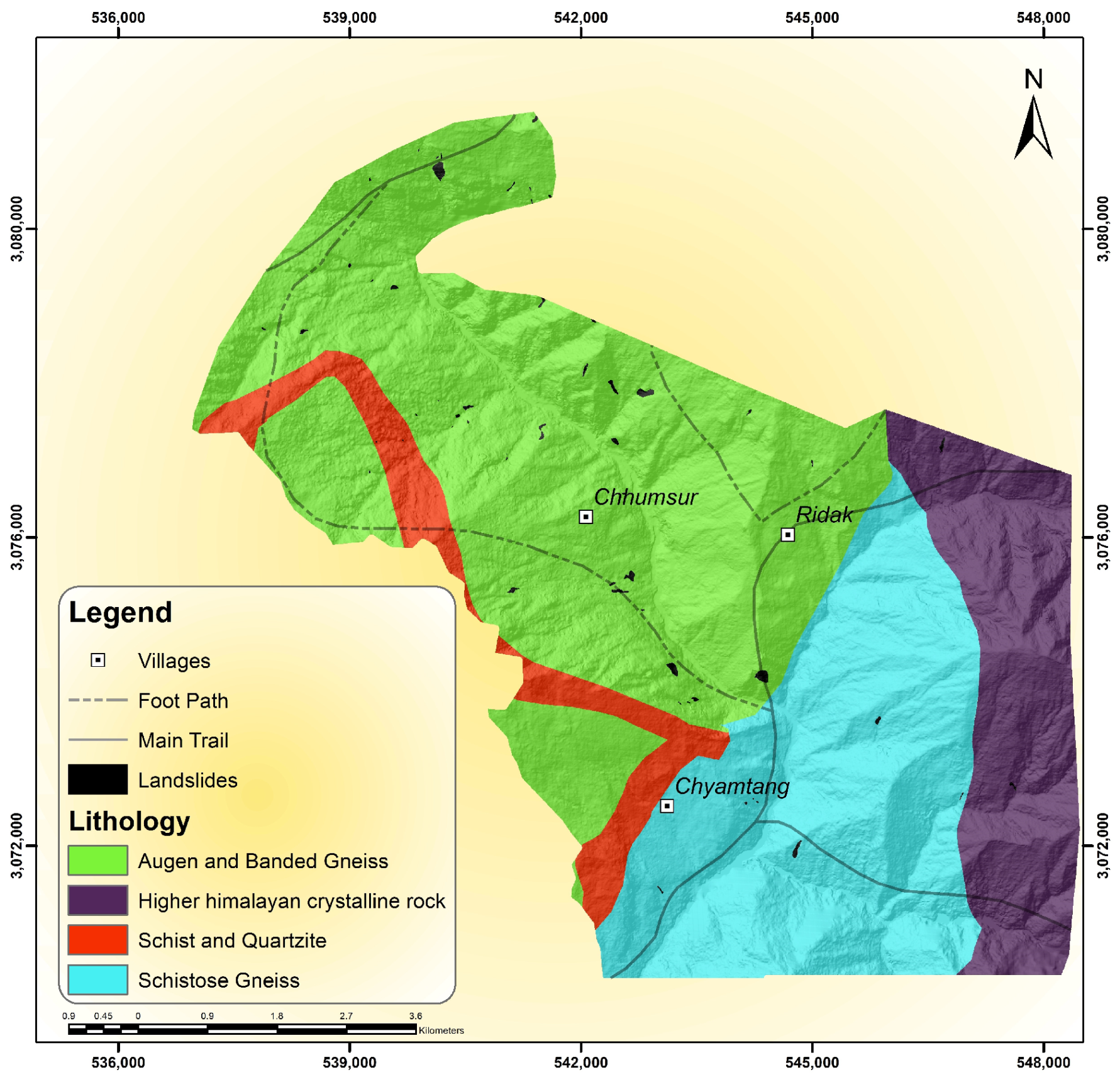
4.1.6. Geology
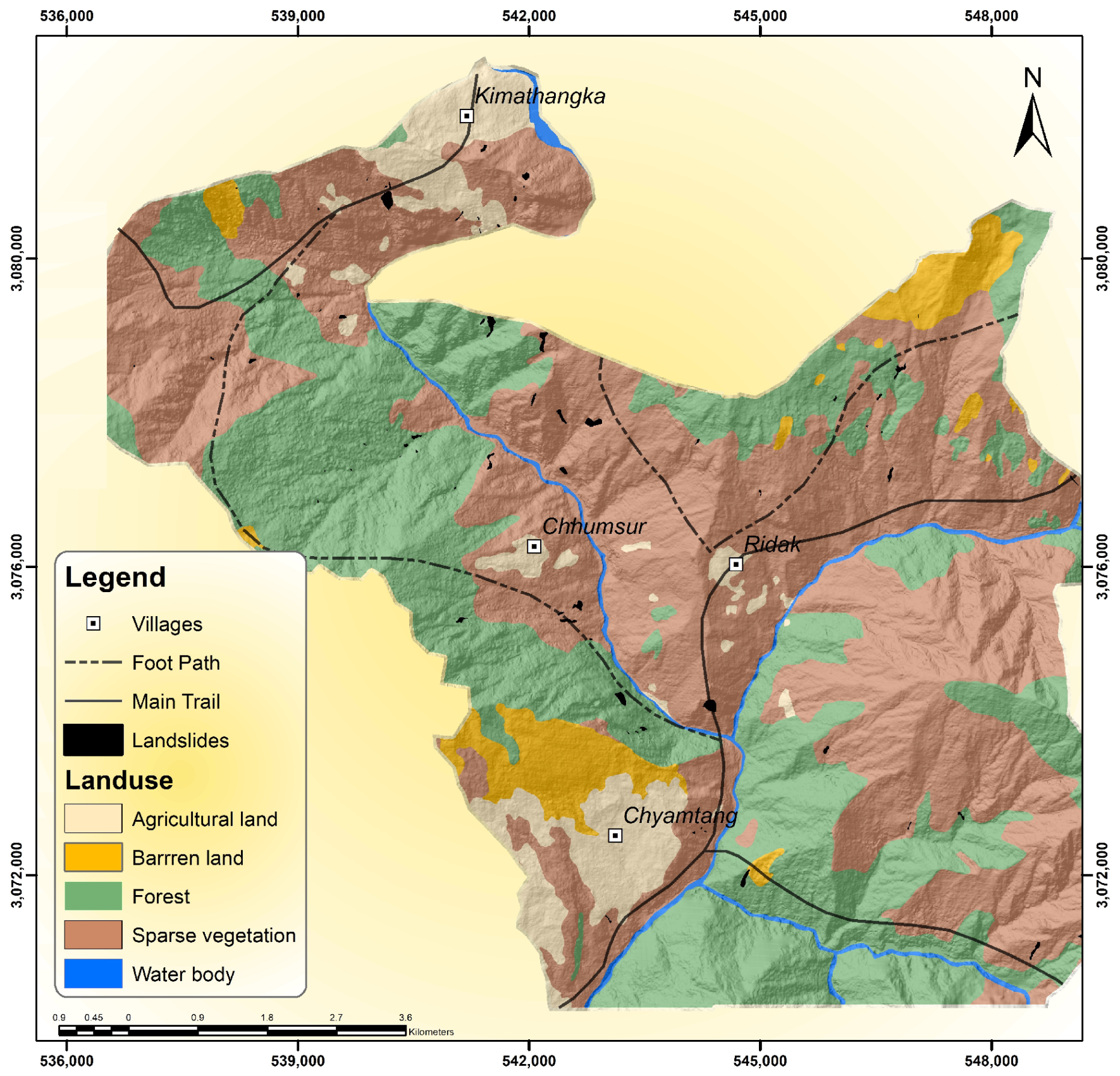
4.1.7. Land Use
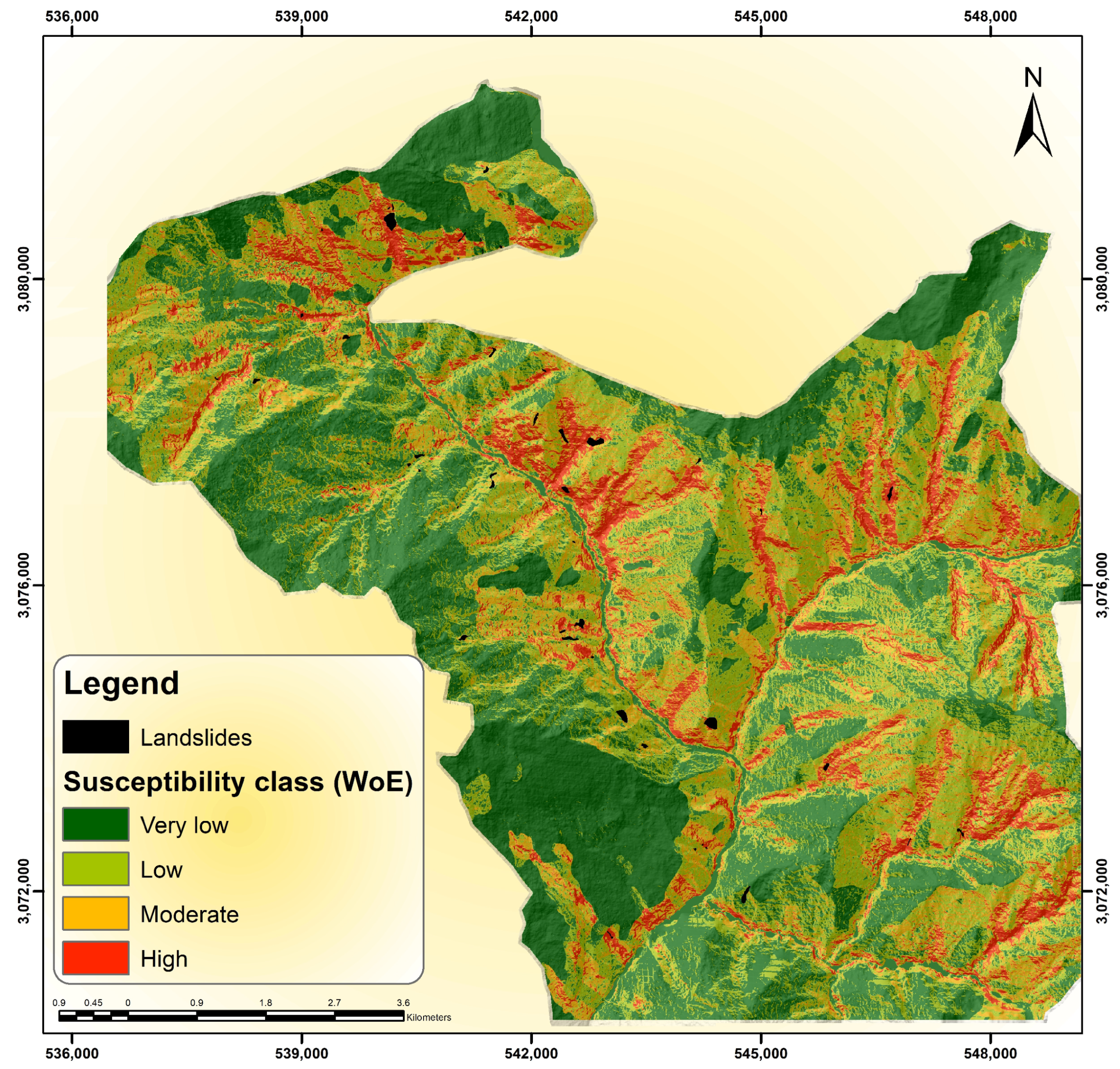
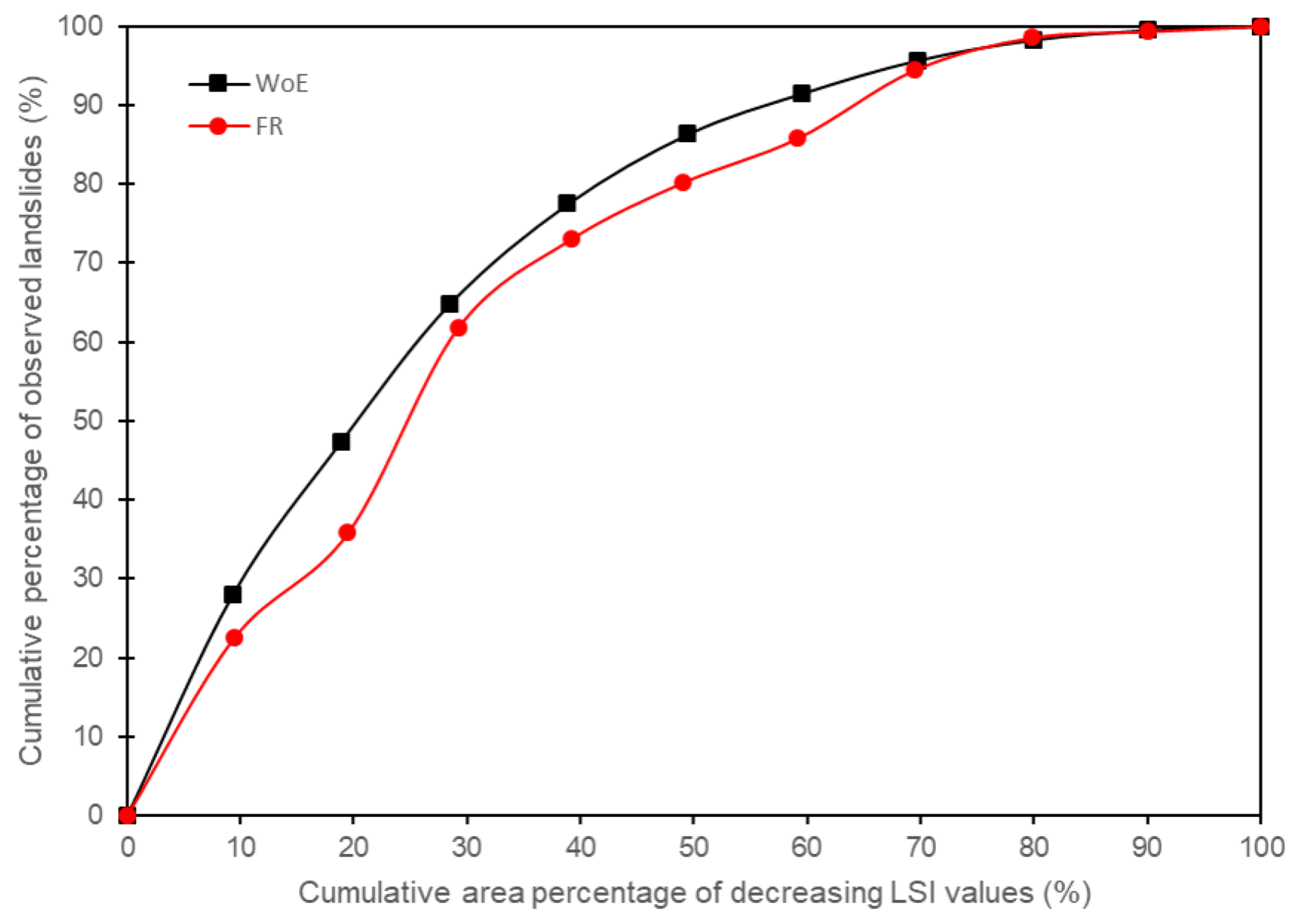
4.2. Assessment Results
5. Discussion
6. Concluding Remarks
Author Contributions
Funding
Institutional Review Board Statement
Informed Consent Statement
Data Availability Statement
Acknowledgments
Conflicts of Interest
References
- Cruden, D.M. A simple definition of a landslide. Bull. Int. Assoc. Eng. Geol. 1991, 41, 27–29. [Google Scholar] [CrossRef]
- Lacasse, S.; Nadim, F. Landslide Risk Assessment and Mitigation Strategy, 1st ed.; Springer: Berlin, Germany, 2009; pp. 30–35. [Google Scholar]
- Petley, D.N.; Hearn, G.J.; Hart, A.; Rosser, N.J.; Dunning, S.A.; Oven, K.; Mitchell, W.A. Trends in landslide occurrence in Nepal. Nat. Hazard. 2007, 43, 23–44. [Google Scholar] [CrossRef]
- Dahal, R.K.; Hasegawa, S. Representative rainfall thresholds for landslides in the Nepal Himalaya. Geomorphology 2008, 100, 429–443. [Google Scholar] [CrossRef]
- Dahal, R.K.; Hasegawa, S.; Nonomura, A.; Yamanaka, M.; Dhakal, S. DEM-based deterministic landslide hazard analysis in the Lesser Himalaya of Nepal. Georisk 2008, 2, 161–178. [Google Scholar] [CrossRef]
- McAdoo, B.G.; Quak, M.; Gnyawali, K.R.; Adhikari, B.R.; Devkota, S.; Rajbhandari, P.L.; Sudmeier-Rieux, K. Roads and landslides in Nepal: How development affects environmental risk. Nat. Hazards Earth Syst. Sci. 2018, 18, 3203–3210. [Google Scholar] [CrossRef] [Green Version]
- Tsou, C.Y.; Chigira, M.; Higaki, D.; Sato, G.; Yagi, H.; Sato, H.P.; Wakai, A.; Dangol, V.; Amatya, S.C.; Yatagaim, A. Topographic and geologic controls on landslides induced by the 2015 Gorkha earthquake and its aftershocks: An example from the Trishuli Valley, central Nepal. Landslides 2018, 15, 953–965. [Google Scholar] [CrossRef]
- Dahal, B.K.; Dahal, R.K. Landslide hazard map: Tool for optimization of low-cost mitigation. Geoenviron. Disasters 2017, 4, 8. [Google Scholar] [CrossRef] [Green Version]
- Dai, F.C.; Lee, C.F.; Ngai, Y.Y. Landslide risk assessment and management: An overview. Eng. Geol. 2002, 64, 65–87. [Google Scholar] [CrossRef]
- Kayastha, P.; Dhital, M.R.; De Smedt, F. Landslide susceptibility mapping using the weight of evidence method in the Tinau watershed, Nepal. Nat. Hazard. 2012, 63, 479–498. [Google Scholar] [CrossRef]
- Forte, G.; De Falco, M.; Santangelo, N.; Santo, A. Slope stability in a multi-hazard eruption scenario (Santorini, Greece). Geosciences 2019, 9, 412. [Google Scholar] [CrossRef] [Green Version]
- Reichenbach, P.; Rossi, M.; Malamud, B.D.; Mihir, M.; Guzzetti, F. A review of statistically-based landslide susceptibility models. Earth Sci. Rev. 2018, 180, 60–91. [Google Scholar] [CrossRef]
- Yan, F.; Zhang, Q.; Ye, S.; Ren, B. A novel hybrid approach for landslide susceptibility mapping integrating analytical hierarchy process and normalized frequency ratio methods with the cloud model. Geomorphology 2019, 327, 170–187. [Google Scholar] [CrossRef]
- Gorsevski, P.V.; Gessler, P.E.; Jankowski, P. Integrating a fuzzy k-means classification and a Bayesian approach for spatial prediction of landslide hazard. J. Geogr. Syst. 2003, 5, 223–251. [Google Scholar] [CrossRef]
- Kaur, H.; Gupta, S.; Parkash, S. Comparative evaluation of various approaches for landslide hazard zoning: A critical review in Indian perspectives. Spat. Inf. Res. 2017, 25, 389–398. [Google Scholar] [CrossRef]
- Wang, Q.; Wang, Y.; Niu, R.; Peng, L. Integration of information theory, K-means cluster analysis and the logistic regression model for landslide susceptibility mapping in the Three Gorges Area, China. Remote Sens. 2017, 9, 938. [Google Scholar] [CrossRef] [Green Version]
- Lee, S. Application of likelihood ratio and logistic regression models to landslide susceptibility mapping using GIS. Environ. Manag. 2004, 34, 223–232. [Google Scholar] [CrossRef]
- Ayalew, L.; Yamagishi, H. The application of GIS-based logistic regression for landslide susceptibility mapping in the Kakuda-Yahiko Mountains, Central Japan. Geomorphology 2005, 65, 15–31. [Google Scholar] [CrossRef]
- Yesilnacar, E.; Topal, T.A.M.E.R. Landslide susceptibility mapping: A comparison of logistic regression and neural networks methods in a medium scale study, Hendek region (Turkey). Eng. Geol. 2005, 79, 251–266. [Google Scholar] [CrossRef]
- Bui, D.T.; Lofman, O.; Revhaug, I.; Dick, O. Landslide susceptibility analysis in the Hoa Binh province of Vietnam using statistical index and logistic regression. Nat. Hazard. 2011, 59, 1413–1444. [Google Scholar] [CrossRef]
- Yang, J.; Song, C.; Yang, Y.; Xu, C.; Guo, F.; Xie, L. New method for landslide susceptibility mapping supported by spatial logistic regression and GeoDetector: A case study of Duwen Highway Basin, Sichuan Province, China. Geomorphology 2019, 324, 62–71. [Google Scholar] [CrossRef]
- Ilia, I.; Tsangaratos, P. Applying weight of evidence method and sensitivity analysis to produce a landslide susceptibility map. Landslides 2004, 13, 379–397. [Google Scholar] [CrossRef]
- Vakhshoori, V.; Zare, M. Landslide susceptibility mapping by comparing weight of evidence, fuzzy logic, and frequency ratio methods. Geomat. Nat. Hazards Risk 2016, 7, 1731–1752. [Google Scholar] [CrossRef]
- Hong, H.; Ilia, I.; Tsangaratos, P.; Chen, W.; Xu, C. Applying weight of evidence method and sensitivity analysis to produce a landslide susceptibility map.A hybrid fuzzy weight of evidence method in landslide susceptibility analysis on the Wuyuan area, China. Geomorphology 2017, 290, 1–16. [Google Scholar] [CrossRef]
- Xie, Z.; Chen, G.; Meng, X.; Zhang, Y.; Qiao, L.; Tan, L. A comparative study of landslide susceptibility mapping using weight of evidence, logistic regression and support vector machine and evaluated by SBAS-InSAR monitoring: Zhouqu to Wudu segment in Bailong River Basin, China. Environ. Earth Sci. 2017, 76, 1–19. [Google Scholar] [CrossRef]
- Lee, S.; Evangelista, D.G. Earthquake-induced landslide-susceptibility mapping using an artificial neural network. Nat. Hazards Earth Syst. Sci. 2006, 6, 687–695. [Google Scholar] [CrossRef]
- Choi, J.; Oh, H.J.; Won, J.S.; Lee, S. Validation of an artificial neural network model for landslide susceptibility mapping. Environ. Earth Sci. 2010, 60, 473–483. [Google Scholar] [CrossRef]
- Chen, W.; Pourghasemi, H.R.; Zhao, Z. A GIS-based comparative study of Dempster-Shafer, logistic regression and artificial neural network models for landslide susceptibility mapping. Geocarto Int. 2017, 32, 367–385. [Google Scholar] [CrossRef]
- Akinci, H.; Doan, S.; Kiliccedil, C.; Temiz, M.S. DProduction of landslide susceptibility map of Samsun (Turkey) City Center by using frequency ratio method. Int. J. Phys. Sci. 2011, 6, 1015–1025. [Google Scholar]
- Park, S.; Choi, C.; Kim, B.; Kim, J. Landslide susceptibility mapping using frequency ratio, analytic hierarchy process, logistic regression, and artificial neural network methods at the Inje area, Korea. Environ. Earth Sci. 2013, 68, 1443–1464. [Google Scholar] [CrossRef]
- Poudyal, C.P.; Chang, C.; Oh, H.J.; Lee, S. Landslide susceptibility maps comparing frequency ratio and artificial neural networks: A case study from the Nepal Himalaya. Environ. Earth Sci. 2010, 61, 1049–1064. [Google Scholar] [CrossRef]
- Kayastha, P.; Dhital, M.R.; De Smedt, F. Evaluation and comparison of GIS based landslide susceptibility mapping procedures in Kulekhani watershed, Nepal. J. Geol. Soc. India 2013, 81, 219–231. [Google Scholar] [CrossRef]
- Bijukchhen, S.M.; Kayastha, P.; Dhital, M.R. A comparative evaluation of heuristic and bivariate statistical modelling for landslide susceptibility mappings in Ghurmi-Dhad Khola, east Nepal. Arabian J. Geosci. 2013, 6, 2727–2743. [Google Scholar] [CrossRef]
- Dahal, R.K. Regional-scale landslide activity and landslide susceptibility zonation in the Nepal Himalaya. Environ. Earth Sci. 2014, 71, 5145–5164. [Google Scholar] [CrossRef]
- Amatya, P.; Kirschbaum, D.; Stanley, T. Use of very high-resolution optical data for landslide mapping and susceptibility analysis along the Karnali highway, Nepal. Remote Sens. 2019, 11, 2284. [Google Scholar] [CrossRef] [Green Version]
- Dhital, M.R. Geology of the Nepal Himalaya; Springer International Publishing: Cham, Switzerland, 2015. [Google Scholar]
- Schelling, D. The tectonostratigraphy and structure of the eastern Nepal Himalaya. Tectonics 1992, 11, 925–943. [Google Scholar] [CrossRef]
- Alaska Satellite Facility. Available online: https://asf.alaska.edu (accessed on 12 October 2021).
- Bonham-Carter, G.F.; Agterberg, F.P.; Wright, D.F. Integration of geological datasets for gold exploration in Nova Scotia. Photogramm. Eng. Remote Sens. 1988, 54, 1585–1592. [Google Scholar]
- Bonham-Carter, G.F. Geographic Information Systems for Geoscientists, Modeling with GIS; Elsevier: Amsterdam, The Netherlands, 1994. [Google Scholar]
- Lee, S.; Pradhan, B. Landslide hazard mapping at Selangor, Malaysia using frequency ratio and logistic regression models. Landslides 2007, 4, 33–41. [Google Scholar] [CrossRef]
- Jadda, M.; Shafri, H.Z.M.; Mansor, S.B.; Sharifikia, M.; Pirasteh, S. Landslide susceptibility evaluation and factor effect analysis using probabilistic-frequency ratio model. Eur. J. Sci. Res. 2009, 33, 654–668. [Google Scholar]
- Yilmaz, I. Landslide susceptibility mapping using frequency ratio, logistic regression, artificial neural networks and their comparison: A case study from Kat landslides (Tokat-Turkey). Comput Geosci. 2009, 35, 1125–1138. [Google Scholar] [CrossRef]
- Lee, S.; Talib, J.A. Probabilistic landslide susceptibility and factor effect analysis. Environ. Geol. 2005, 47, 982–990. [Google Scholar] [CrossRef]
- Gyawali, P.; Aryal, Y.M.; Tiwari, A.; Prajwol, K.C.; Ansari, K. Landslide Susceptibility Assessment Using Bivariate Statistical Methods: A Case Study of Gulmi District, western Nepal. VW Eng. Int. 2021, 3, 29–40. [Google Scholar]
- Dangi, H.; Bhattarai, T.N.; Thapa, P.B. An approach of preparing earthquake induced landslide hazard map: A case study of Nuwakot District, central Nepal. Nepal Geol. Soc. 2019, 58, 153–162. [Google Scholar] [CrossRef]
- Gokceoglu, C.; Aksoy, H. Landslide susceptibility mapping of the slopes in the residual soils of the Mengen region (Turkey) by deterministic stability analyses and image processing techniques. Eng. Geol. 1996, 44, 147–161. [Google Scholar] [CrossRef]
- Kanungo, D.P.; Singh, R.; Dash, R.K. Field observations and lessons learnt from the 2018 landslide disasters in Idukki District, Kerala, India. Curr. Sci. 2020, 119, 1797. [Google Scholar] [CrossRef]
- Yalcin, A.; Bulut, F. Landslide susceptibility mapping using GIS and digital photogrammetric techniques: A case study from Ardesen (NE-Turkey). Nat. Hazards 2007, 41, 201–226. [Google Scholar] [CrossRef]
- Yalcin, A. GIS-based landslide susceptibility mapping using analytical hierarchy process and bivariate statistics in Ardesen (Turkey): Comparisons of results and confirmations. Catena 2008, 72, 1–12. [Google Scholar] [CrossRef]
- Van Westen, C.J.; Rengers, N.; Soeters, R. Use of geomorphological information in indirect landslide susceptibility assessment. Nat. Hazards 2003, 30, 399–419. [Google Scholar] [CrossRef]
- Akgun, A. A comparison of landslide susceptibility maps produced by logistic regression, multi-criteria decision, and likelihood ratio methods: A case study at Izmir, Turkey. Landslides 2012, 9, 93–106. [Google Scholar] [CrossRef]


| Slope Angle | Area | Landslides | C | ||||
|---|---|---|---|---|---|---|---|
| Class | (Pixels) | (Pixels) | |||||
| 0∼ | 202,156 | 60 | −2.2978 | 0.0508 | −2.3486 | 0.1295 | −18.1398 |
| 15∼ | 563,158 | 533 | −1.1376 | 0.1153 | −1.2529 | 0.0444 | −28.1940 |
| 25∼ | 1,019,975 | 1820 | −0.5026 | 0.1402 | −0.6429 | 0.0257 | −25.0063 |
| 35∼ | 993,193 | 2970 | 0.0149 | −0.0055 | 0.0204 | 0.0215 | 0.9489 |
| 45∼ | 591,787 | 2805 | 0.4773 | −0.1235 | 0.6008 | 0.0220 | 27.3653 |
| 55∼ | 258,830 | 1855 | 0.8932 | −0.1143 | 1.0075 | 0.0256 | 39.4025 |
| > | 71,924 | 861 | 1.4111 | −0.0628 | 1.4739 | 0.0357 | 41.2706 |
| Zone | Area | Landslides | Landslide Density | ||
|---|---|---|---|---|---|
| Value () | Percentage (%) | Value () | Percentage (%) | (%) | |
| very low | 37,095,800 | 40.48 | 23,150 | 8.51 | 0.06 |
| low | 28,432,150 | 31.02 | 72,425 | 26.61 | 0.25 |
| moderate | 17,555,600 | 19.16 | 100,150 | 36.80 | 0.57 |
| high | 8,563,550 | 9.34 | 76,400 | 28.08 | 0.89 |
| Zone | Area | Landslides | Landslide Density | ||
|---|---|---|---|---|---|
| Value () | Percentage (%) | Value () | Percentage (%) | (%) | |
| very low | 37,458,375 | 40.87 | 38,650 | 14.20 | 0.10 |
| low | 27,414,225 | 29.91 | 65,200 | 23.96 | 0.24 |
| moderate | 18,060,200 | 19.71 | 106,700 | 39.21 | 0.59 |
| high | 8,714,300 | 9.51 | 61,575 | 22.63 | 0.71 |
Publisher’s Note: MDPI stays neutral with regard to jurisdictional claims in published maps and institutional affiliations. |
© 2022 by the authors. Licensee MDPI, Basel, Switzerland. This article is an open access article distributed under the terms and conditions of the Creative Commons Attribution (CC BY) license (https://creativecommons.org/licenses/by/4.0/).
Share and Cite
KC, D.; Dangi, H.; Hu, L. Assessing Landslide Susceptibility in the Northern Stretch of Arun Tectonic Window, Nepal. CivilEng 2022, 3, 525-540. https://doi.org/10.3390/civileng3020031
KC D, Dangi H, Hu L. Assessing Landslide Susceptibility in the Northern Stretch of Arun Tectonic Window, Nepal. CivilEng. 2022; 3(2):525-540. https://doi.org/10.3390/civileng3020031
Chicago/Turabian StyleKC, Diwakar, Harish Dangi, and Liangbo Hu. 2022. "Assessing Landslide Susceptibility in the Northern Stretch of Arun Tectonic Window, Nepal" CivilEng 3, no. 2: 525-540. https://doi.org/10.3390/civileng3020031