Comparison of Multi-Criteria Group Decision-Making Methods for Urban Sewer Network Plan Selection

Abstract

Selecting a suitable sewer network plan for a city is a complex and challenging task that requires discussion among a group of experts and the consideration of multiple conflicting criteria with different measurement units. A number of multi-criteria decision-making (MCDM) methods have been proposed for analyzing sewer network selection problems, each having their own distinct advantages and limitations. Although many decision-making techniques are available, decision-makers are confronted with the difficult task of selecting the appropriate MCDM method, as each method can lead to different results when applied to an identical problem. This paper evaluates four different multi-criteria decision-making methods, which are the Analytic Hierarchy Process (AHP), the Technique for Order Preference by Similarity to Ideal Solution (TOPSIS), Elimination Et Choix Traduisant la REalité (ELECTRE III) and the Preference Ranking Organization METHods for Enrichment Evaluations II (PROMETHEE II), for one sewer network group decision problem in the early stage of sewer water infrastructure asset management. Moreover, during the implementation of different MCDM methods, the Delphi technique is introduced to organize and structure the discussions among all the decision-makers. The results of the study are examined based on each method’s ability to provide accurate representations of the decision-makers’ preferences and their experience implementing each method. As a conclusion, decision-makers identify PROMETHEE II as their favorite method, AHP is more time and energy consuming and results in a number of inconsistencies, while TOPSIS loses information during vector normalization for multi-dimension criteria, and ELECTRE III’s results are inconclusive.

1. Introduction

A sewer network system is the infrastructure that transports sewage, rainwater or stormwater. The main part of this system encompasses components such as manholes, pumping stations and large pipes in a combined sewer (sewage and rainwater) or sanitary sewer (sewage only) system. Sewer water infrastructure asset management has major impacts on protecting public health and sustaining our environments [1,2,3]. Deciding on the right sewer network plan is challenging, especially when considering the following requirements [4]: first, the selected sewer system plan’s quality, life-cycle maintenance and performance need to meet the sustainability requirements for society, the economy, and the environment [5]; second, the decision should involve all the stakeholders’ preferences [6]; third, the decision-making must incorporate uncertainty, i.e., information is imperfect or unknown [7]; fourth, long-term planning for future climate change, urban development in the context of population increase or decrease, and numerous environmental pollutants, etc., must be a factor.

Multi-criteria decision-making (MCDM) is able to meet all the above challenges [8,9]. It is a procedure that structures and solves decision problems by combining the performance of each decision alternative for multiple conflicting, qualitative and/or quantitative decision criteria and outcomes into a compromise choice. The relevant MCDM methods have been developed to help decision-makers solve MCDM problems. They are widely applied in different types of real-life problems where groups of decision alternatives are considered against conflicting criteria [10]. The application of MCDM methods in water and wastewater infrastructure management has steadily increased in the literature since 1990—the analytic hierarchy process (AHP) [11], the ELimination Et Choix Traduisant la REalité (ELECTRE) [12], the Preference Ranking Organization METHods for Enrichment Evaluations (PROMETHEE) [13], and the Technique for Order Preference by Similarity to Ideal Solution (TOPSIS) [14] are the most widely employed of all the various MCDM methods [15].

Due to the number of MCDM methods available, decision-makers are confronted by the difficult task of selecting the appropriate MCDM method, as each method has its own limitations, particularities, hypotheses, premises and perspectives and can lead to different results when applied to an identical problem [16]. Hence, it is worth evaluating the performance of different methods using a single decision problem. The aim of this paper is to present a comparative study of the most applied MCDM methods in the field of water and wastewater infrastructure management (AHP, ELECTRE, PROMETHEE, TOPSIS) by applying them to one real-world sewer network planning case study and analyzing the suitability of results in order to highlight the differences and reach meaningful conclusions.

The comparative study among different multi-criteria decision-making methods is a popular research topic. Different groups of MCDM methods are compared and applied in different practical implementation areas, which brings different insights. The most recent research on this topic are: the work of [17], a comparative analysis among MOORA (Multi-Objective Optimization on the basis of Ratio Analysis), TOPSIS and VIKOR methods (the compromise ranking method) for selecting the best material for braking booster valve body; [18], whose research incorporates AHP, MARE and ELECTRE III to deal with equipment selection task; [19], who compared Simple Additive Weighting Method, Weighted product method, AHP and TOPSIS for the energy demand planning; and [20], who carried out a study among MAUT, AHP and TOPSIS on the application of a gender inequality index.

The rest of the paper is organized as follows: Section 2 presents an overview of each selected MCDM method with a detailed description of their processes; Section 3 describes the implementation process of each MCDM method in one sewer network planning case study and provides a comparative analysis of the results; Section 4 offers the conclusion and suggestions for future work.

2. Overview of Selected Multi-Criteria Methods

A good number of multi-criteria decision-making methods have been developed to provide techniques for decision-makers during the decision process. They incorporate all the objective and subjective information in order to find a compromise optimal solution. According to the literature, the available methods can be grouped into three categories [16,21]:

• Full aggregation methods: each criterion is assigned a weight, which indicates the importance of the criterion, then a numerical score for each alternative is calculated and the one with highest score prevails (e.g., AHP).
• Outranking methods: each pair of alternatives is compared for each criterion to rank the alternatives (e.g., ELECTRE, PROMETHEE).
• Goal, aspiration or reference level methods: these methods identify how far each alternative is from the ideal goal or aspiration (e.g., TOPSIS).

For the purpose of this paper, the following methods are reviewed and selected, as they are MCDM methods widely used in decision problems for water and wastewater infrastructure management: AHP, ELECTRE, PROMETHEE and TOPSIS.

2.1. AHP

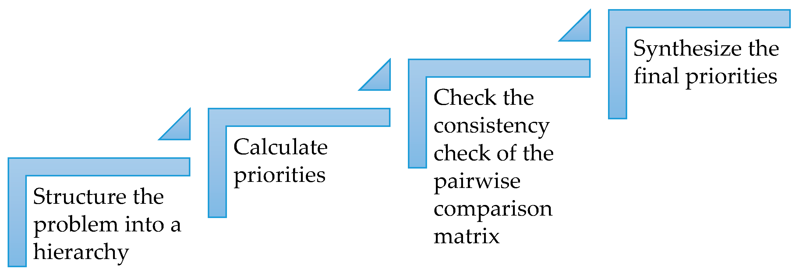
The analytic hierarchy process (AHP), from the group of full aggregation methods, was developed by Thomas L. Saaty in 1980 [11,22]. In general, AHP contains four steps, as shown in Figure 1.

The first step involves structuring the original decision problem into a hierarchical structure. The overall goal of the problem is at the top level of the hierarchy; the next level contains the criteria representing the different dimensions from which the alternatives can be considered; the bottom level is filled with decision alternatives, which are the different choices available to the decision-maker. The second step is to calculate the priority of each criterion with respect to the goal and the priority of each alternative with respect to one specific criterion. The technique of pairwise comparison with a 1–9 fundamental scale [23], shown in

Table 1. The fundamental scale for pairwise comparison in AHP.

Degree of Importance	Definition	Explanation
1	Equal importance	Two candidates contribute equally to the objective.
3	Moderate importance	Experience and judgment slightly favor one candidate over another.
5	Strong importance	Experience and judgment strongly favor one candidate over another.
7	Very strong importance	One candidate is favored very strongly over another.
9	Extreme importance	The evidence favoring one candidate over another is of the highest possible order of affirmation.
Degrees of 2, 4, 6 and 8 can be used to express intermediate values. Degrees of 1.1, 1.2, 1.3, etc. can be used for alternatives that are very close in importance.

, is used to obtain pairwise comparison matrix $S=\left(s_{ij}\right)$, which is a positive reciprocal matrix, i.e., $s_{ji}=\frac{1}{s_{ij}}$. Saaty proves that the principal right eigenvector of $S$ sufficiently represents the priority vector when $S$ is a small perturbation of a consistent matrix [24]. Hence, the third step is to perform a consistency check of pairwise comparison matrices. This requires computing the consistency index ($CI$) by: $=\frac{{\lambda }_{max}-n}{n-1}$, where ${\lambda }_{max}$ is the largest eigenvalue of the matrix and $n$ is the number of independent rows in the matrix. Then the random index $RI$, which is the average $CI$ values from a random simulation of pairwise comparison matrices (

Table 2. Random Index (RI) for different values of n [25].

Number of Rows in the Matrix	3	4	5	6	7	8	9	10
$RI$	0.525	0.880	1.109	1.248	1.342	1.406	1.450	1.485

) is introduced. If $\frac{CI}{RI}\le 0.1$, the inconsistency is acceptable; if $\frac{CI}{RI}>0.1$, the subjective pairwise comparison judgment needs to be revised. The last step is to summarize a set of overall priorities in order to make the final decision. The alternative with the highest priority with respect to the goal is considered the final decision choice.

AHP has received the most academic attention and been frequently used around the world in a large variety of applications due to its simplicity, ease to understand and the quality assurance provided by the consistency check. AHP is used in 28.3% of publications regarding water and wastewater [15,26]. The disadvantages of AHP are: the potential compensation between good scores on some criteria and bad scores on others causes the loss of information [27]; and the complexity and time of computation depends on the number of criteria and alternatives [28].

2.2. TOPSIS

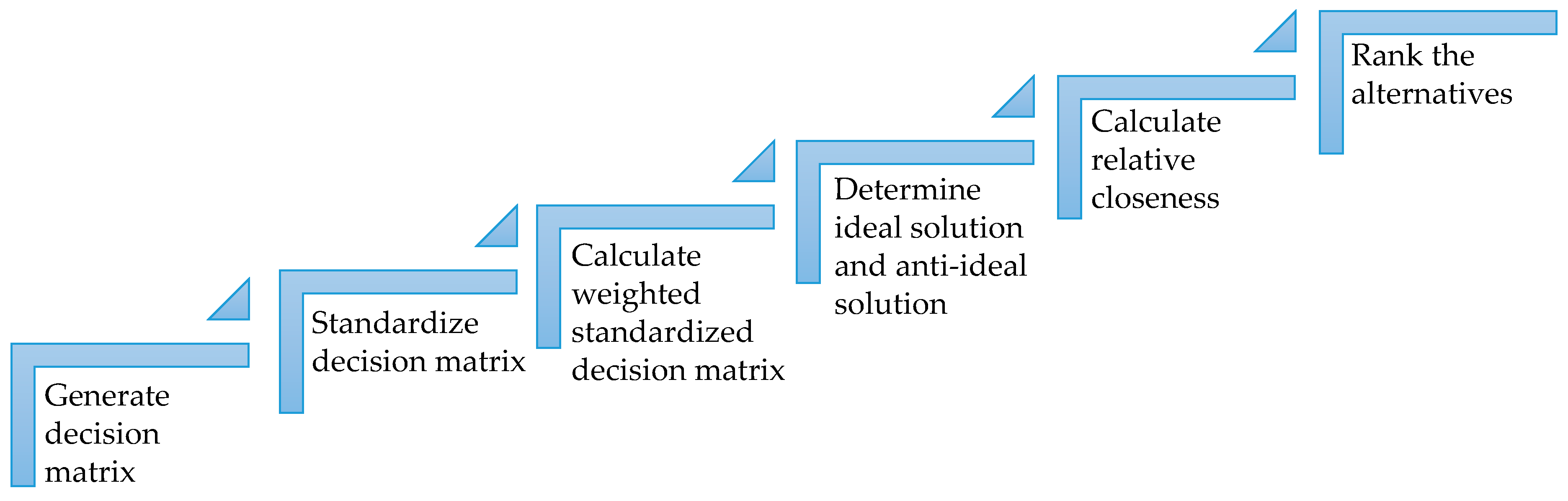
The Technique for Order of Preference by Similarity to Ideal Solution (TOPSIS), from the group of goal, aspiration or reference level methods, was first presented by Hwang and Yoon in 1981 [29]. The basic principle of this method is that the optimal alternative is the one that is the shortest distance to the ideal solution and the furthest distance from the anti-ideal solution [15,16]. The ideal solution maximizes the benefit criteria and minimizes the cost criteria, whereas the anti-ideal solution maximizes the cost criteria and minimizes the benefit criteria [15,30].

As shown in Figure 2, the TOPSIS process first generates the decision matrix $A={\left(a_{ij}\right)}_{m\times n}$ which contains m alternatives, denoted as $d_1, d_2, \dots , d_m$, and $n$ criteria, denoted as $c_1, c_2, \dots , c_n$, with the intersection of each alternative and criterion given as $a_{ij}$. Then, it calculates the standardized matrix $R={\left(r_{ij}\right)}_{m\times n}$ using the following equation:

$$r_{ij}=\frac{a_{ij}}{\sqrt{{{\displaystyle \sum }}_{k=1}^m{a}_{kj}^2}} , i=1,2,\cdots ,m, j=1,2,\cdots ,n.$$

(1)

and the weighted standardized matrix $T={\left(t_{ij}\right)}_{m\times n}$ by:

$$t_{ij}=r_{ij}·{\omega }_{j }, i=1,2,\cdots ,m, j=1,2,\cdots ,n$$

(2)

where ${\omega }_1, {\omega }_2, \cdots ,{\omega }_n$ is a set of weights associated with the criteria and ${{\displaystyle \sum }}_{j=1}^n{\omega }_j=1$.

The ideal solution $S^{+}$ and the anti-ideal solution $S^{-}$ are defined as follows:

$$S^{+}=\left\{t_j^{+}|j=1,2,\cdots ,n\right\}=\left\{\left(\underset{i}{\min } t_{ij}|j\in J^{-}\right), \left(\underset{i}{\max } t_{ij}|j\in J^{+}\right)\right\},$$

(3)

$$S^{-}=\left\{t_j^{-}|j=1,2,\cdots ,n\right\}=\left\{\left(\underset{i}{\max } t_{ij}|j\in J^{-}\right), \left(\underset{i}{\min } t_{ij}|j\in J^{+}\right)\right\},$$

(4)

where $J^{+}$ and $J^{-}$ are related to the benefit and cost criteria, respectively.

Then, compute the $n$-dimensional Euclidean distance from the alternative $i$ to the ideal solution $S^{+}$ and the anti-ideal solution $S^{-}$, denoted as $D_i^{+}$ and $D_j^{-}$ in the following equations:

$$D_i^{+}=\sqrt{{\displaystyle \sum }_{j=1}^n{\left(t_{ij}-t_j^{+}\right)}^2}$$

(5)

$$D_i^{-}=\sqrt{{\displaystyle \sum }_{j=1}^n{\left(t_{ij}-t_j^{-}\right)}^2}$$

(6)

Each alternative’s relative closeness to the ideal solution is obtained by:

$$C_i=\frac{D_i^{-}}{\left(D_i^{+}+D_i^{-}\right)}$$

(7)

If $C_i=1$, alternative $i$ is the ideal solution, if $C_i=0$, alternative $i$ is the anti-ideal solution. The final step is to rank the alternatives based on the values of $C_i$. The maximum value is the best solution to the problem.

The advantage of this method is that it requires only a few inputs from the decision-maker and its output is easy to understand. The drawback is that vector normalization is needed to solve multi-dimensional problems [15]. The application of this method in water and wastewater management can be found in Afshar, Marino and Saadatpour [31] in their ranking of projects in the Karun river basin, Coutinho-Rodrigues, Simao and Antunes [32] in their selection of water supply system investment options for an urban development/expansion project, and Srdjevic, Mederios and Faria [33] in their ranking of water management scenarios.

2.3. ELECTRE

One of the most famous outranking methods is ELimination Et Choix Traduisant la REalité (ELECTRE). The ELECTRE is a family of MCDM methods containing ELECTRE I, ELECTRE II, ELECTRE III, ELECTRE IV, ELECTRE IS and ELECTRE TRI. The two main procedures in ELECTRE methods are: a multiple-criteria aggregation procedure that builds one or several outranking relation(s) in order to compare each pair of alternatives in a comprehensive way; an exploitation procedure that can provide results based on how the problem is being addressed, choosing, ranking or sorting [34]. ELECTRE I was first presented by B. Roy in 1968 [35], which triggered the development of other ELECTRE methods in order to deal with different types of decision problems: ELECTRE I is made for selection problems; ELECTRE TRI for assignment problems; and ELECTRE II, III and IV for ranking problems. 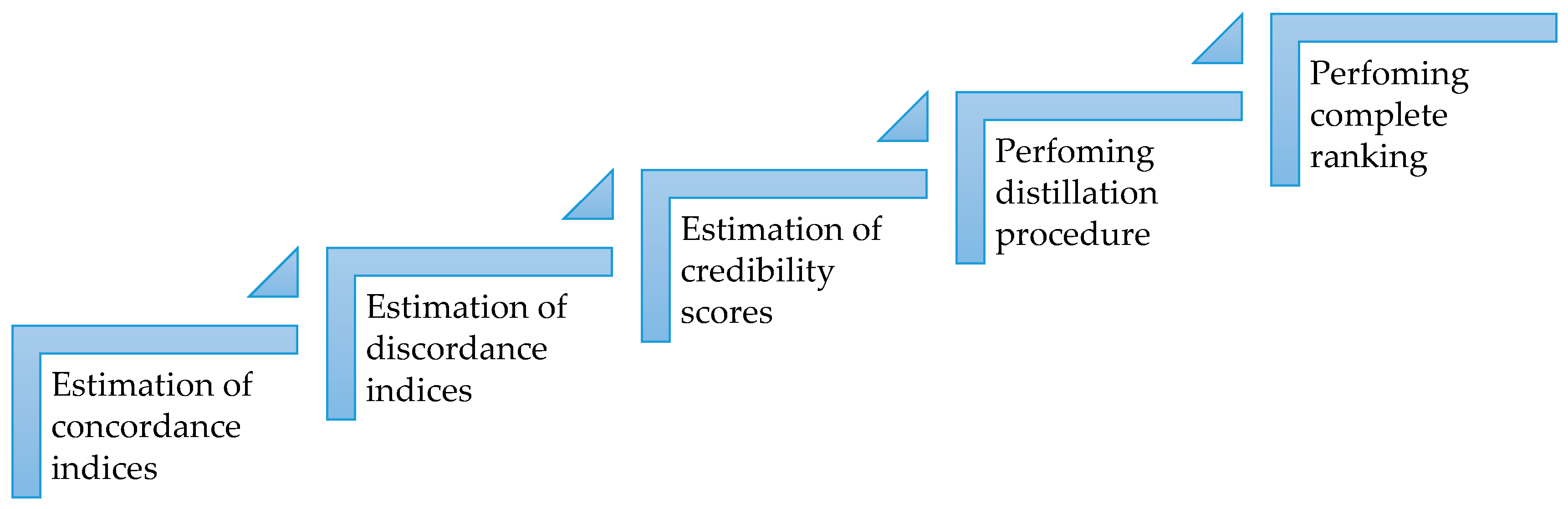ELECTRE III is the most popular of the ELECTRE methods and a well-established partial ranking method, as it considers imprecise data and uncertainties [15,36] and has many successful real-world applications such as environmental and energy management [34,37] strategic planning [38], water and wastewater management [39]. ELECTRE III is selected for this paper. The process of ELECTRE III, as described in Marzouk [40], is given hereafter. To use ELECTRE III, decision-makers need to define criteria indifference $\left(q\right),$ preference $\left(p\right)$, and veto $\left(v\right)$ thresholds where $\left(v\ge q\ge p\right)$ and the weight $\left(w_j\right)$ for each criterion $j$. The main steps used in ELECTRE III are shown in Figure 3. The concordance index, denoted as $C\left(a, b\right)$, is evaluated by an overall comparison of the performances of each pair of $a$ and $b$ alternatives for all criteria. It varies from 0 to 1; a value of 0 means that alternative a is worse than alternative b for all criteria. The concordance index is computed by a weighted comparison of the performances for each criterion $c_j\left(a,b\right)$ individually:

$$C\left(a,b\right)=\frac{1}{W}{\displaystyle \sum }_{j=1}^n{w}_j{c}_j\left(a,b\right), where W={\displaystyle \sum }_{j=1}^n{w}_j$$

(8)

The discordance index for one criterion $j$, denoted as $D_j\left(a,b\right)$, describes the situation where alternative $a$ is better than $b$ generally, but for criterion $j$, alternative $a$ is worse than $b$.

The estimation of credibility scores is based on the concordance and discordance indices in one of the following two scenarios:

• The degree of outranking is equal to the concordance index if there is no criterion that is discordant or where no veto threshold is used;
• The degree of outranking is equal to the concordance with a reduction as the level of discordance increases above a threshold value.

The distillation procedure comprises two parts: descending distillation, where the alternatives are ordered from the best rankings to the worst; ascending distillation which is to order the alternatives from the worst rankings to the best. The final complete ranking result comes from the combination of descending distillation and ascending distillation.

The main advantages of ELECTRE methods is that they avoid compensation between criteria and any normalization process, which distorts the original data. The drawback is that they require various technical parameters, so it is not always easy to fully understand them [16]. ELECTRE methods have been applied in approximately 15.1% of publications regarding water and wastewater: Carriço, Covas, Almeida, Leitao and Alegre [39] used ELECTRE TRI and ELECTRE III to prioritize rehabilitation interventions in the sanitary sewer system in Lisbon; Trojan and Morais [41] applied ELECTRE II to prioritize alternatives for the maintenance of water distribution networks; ELECTRE I was implemented in Morais and Almeida [42] (2006) for the decision on a city’s water supply system.

2.4. PROMETHEE

The Preference Ranking Organization METHods for Enrichment Evaluations (PROMETHEE), another family of outranking methods, ranks alternatives by computing a positive outranking flow and a negative outranking flow for each alternative. Seven different methods in the PROMETHEE group have been developed and used by decision-makers. PROMETHEE I (partial ranking) and PROMETHEE II (complete ranking) were first published in 1982 by Brans [43], then in 1985, Brans and Mareschal developed PROMETHEE III (ranking based on intervals) and PROMETHEE IV (continuous case) [13]. They subsequently suggested PROMETHEE GAIA which provides geometrical representation in support of the PROMETHEE methodology in 1988 [44]. In 1992 and 1995, the same authors proposed another two versions: PROMETHEE V (including segmentation constraints) [45] and PROMETHEE VI (representation of the human brain) [46].

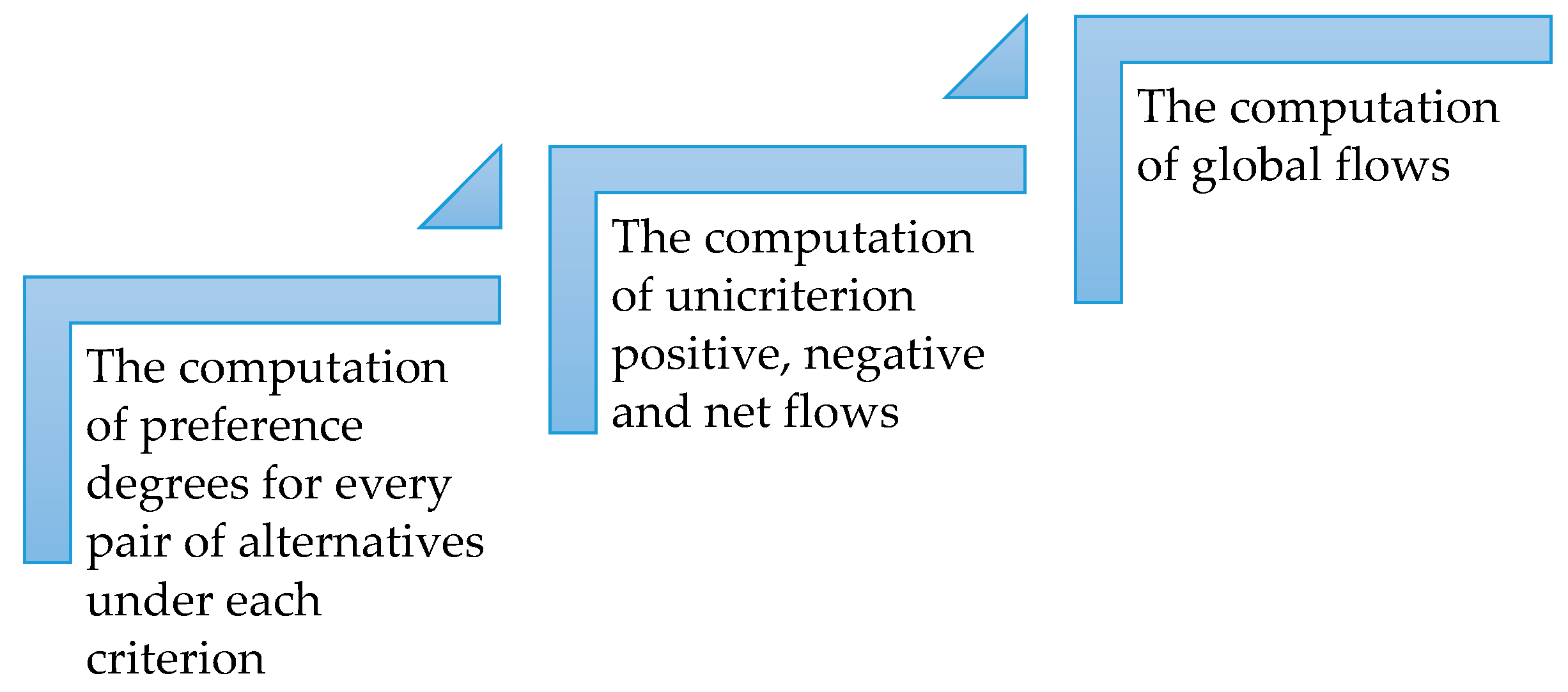
PROMETHEE methods have three main steps [16], as shown in Figure 4.

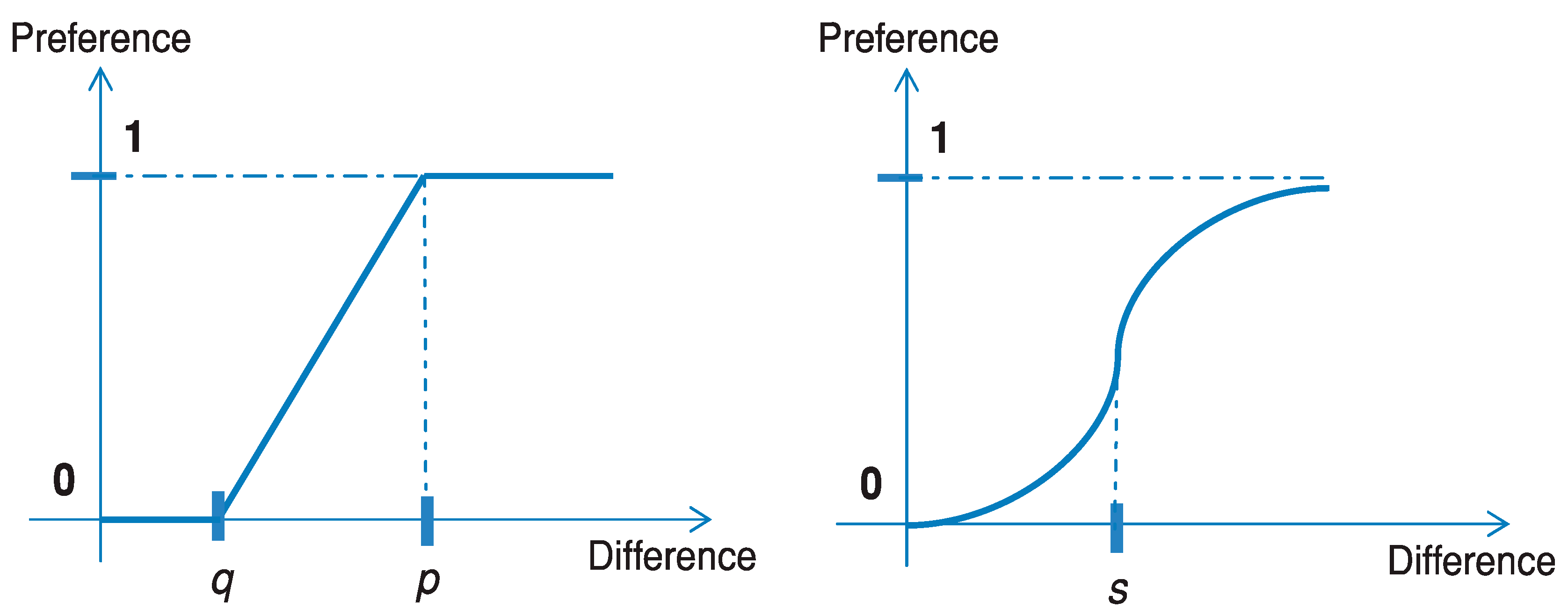
First, the decision-maker looks into each pair of alternatives for one criterion and computes the unicriterion pairwise preference degree, which is a score (between $0$ and $1$) that determines that the decision-maker prefers one alternative over another for the considered criterion. There are two types of preference functions: linear and Gaussian, as shown in Figure 5. The linear preference function requires two parameters: an indifference threshold $q$ and preference threshold $p$; the Gaussian function requires one parameter: the inflexion point $s$.

With the unicriterion pairwise preference degree, it is hard to determine the ranking of all the alternatives, especially when there are many. Therefore, it is necessary to summarize all the unicriterion pairwise preference degrees into unicriterion positive, negative and net flows, which show that an alternative is preferred over all other alternatives.

• A unicriterion positive flow of an alternative is a score between $0$ and $1$, which expresses that an alternative is preferred (based on the decision-maker’s preference) over all other alternatives on that particular criterion. The higher the positive flow, the better the action compared to the others.
• A unicriterion negative flow of an alternative is a score between $0$ and $1$, which expresses that other alternatives are preferred to this one. Note that the unicriterion negative flow needs to be minimized since it represents the weakness of an alternative compared to the other alternatives.
• The unicriterion net flow is based on both positive flow and negative flow. Specifically, an alternative’s net flow is calculated by subtracting the negative flows from the positive flows. These values have to be maximized since they represent the balance between the general strength and the general weakness of an alternative.

In the previous steps, only one criterion is considered at a time. Now, all the criteria are taken into account at the same time in order to compute the global flow. To do so, decision-makers first need to define the relative importance or weight of each criterion $w_j$, where ${{\displaystyle \sum }}_{j=1}^n{w}_j=1$. Then, the weighted sum of all the unicriterion positive, negative and new flows are calculated into global positive, negative and net flows.

• A global positive flow indicates that an alternative is globally preferred to all the other alternatives when considering all the criteria. Since the criteria weights are normalized, the global positive flow is always between $0$ and $1$.
• A global negative flow indicates that other alternatives are preferred over a given alternative. It is between $0$ and $1$ and must be minimized.

The global net flow is obtained by subtracting the global negative flow from the positive flow. The PROMETHEE I ranking depends on the global positive and global negative flows. The PROMETHEE II ranking is based on the global net flows only. In this paper, PROMETHEE II is used. In PROMETHEE II, alternatives can be ranked from the best to the worst, which results in a complete ranking of the alternatives.

The PROMETHEE method allows direct operation on the variables included in the decision matrix without requiring any normalization and is applicable even when there is insufficient information. However, its main drawback is that it is time consuming and difficult for decision-makers to have a clear view of the problem, especially when there are many criteria involved [15,47].

PROMETHEE methods have been applied in 13.2% of publications regarding water and wastewater: Morais and De Almeida [48] used PROMETHEE V to rank alternative strategies for municipal water distribution systems to reduce leakage; PROMETHEE II was applied in Khelifi, Lodolo, Vranes, Centi and Miertus [49] to select groundwater remediation technologies.

3. Case Study

This case study was provided by the civil engineering team from the city of Trois-Rivières. Eight professionals participated in structuring and analyzing the decision problem: one project manager, two civil engineers, two sanitary engineers, two road operators and one environment/weather expert. The decision problem is to select the optimal construction plan to reduce the rainfall flow channeled to the pumping station so that it can accommodate a greater sanitary flow.

3.1. Structuring the Decision Problem

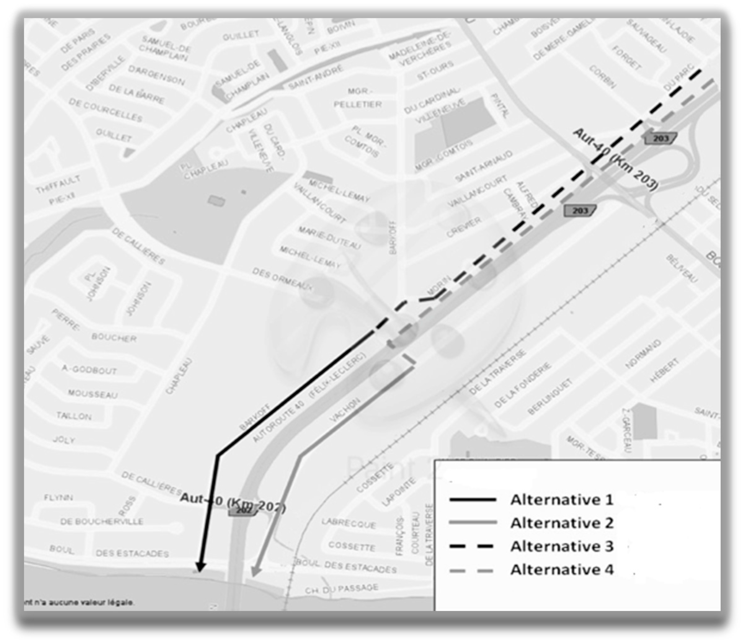
To meet the goal, a rainfall water pipe needs to be designed to guide the water to the local river instead of the pumping station. Civil engineers and sanitary engineers propose four designs; they are referred to as alternatives 1, 2, 3 and 4. Alternatives 1 and 2 are the short-term plans, while alternatives 3 and 4 are their respective long-term extensions. A short description of the four alternatives follows. In Figure 6, Alternative 1 is represented by a black solid line, which is to build a new rainfall water pipe along Barkoff Street from Boulevard des Ormeaux flowing directly to the river; Alternative 2 is to extend the existing rainfall water pipe along rue Vachon to the river, represented by the grey solid line; Alternative 3 includes the construction of Alternative 1, but will further extend the rainfall pipe to the northeast to du Parc Road, represented by the black solid and dashed line; Alternative 4 includes the construction of Alternative 2, while extending the rainfall pipe to the northeast along Morin Road and Highway 40, represented by the grey solid and dashed line.

The Delphi method is applied during the criteria-identification process. The Delphi method, introduced by Dalkey [50], is a structured communication technique to extract and refine group judgments. The Delphi method uses three essential elements: anonymous response, iteration and controlled feedback, and statistical group responses. The eight experts answer the questionnaire in two or more rounds. After each round, each expert revises his/her previous answers based on the anonymized summary of the previous round until a stable result is achieved. Ultimately, five criteria are identified on which to base their decision (see

Table 3. The criteria for the case study.

		Source	Status	Aim
C1	Dynamic performance	Quantitative	Positive	Maximize
C2	Cost of construction	Quantitative	Negative	Minimize
C3	Cost of maintenance	Qualitative	Negative	Minimize
C4	Environmental impact	Qualitative	Negative	Minimize
C5	Potential future profit	Qualitative	Positive	Maximize

).

• Dynamic performance is a positive quantitative variable, and it represents qualitatively how much rainfall flow volume can be reduced in the pumping station (

  Table 4. The dynamic performance of alternatives.

  Alternatives	Dynamic Performance (L/s)
  P1	196.41
  P2	75.64
  P3	214.34
  P4	105.87

  ).
• The cost of construction is a negative quantitative variable defining how much it costs to implement a plan. It covers the cost of the duration of work, manpower, materials, and machines, etc. (

  Table 5. The cost of construction.

  Plan	Total Cost (CAD)
  P1	1,884,753
  P2	437,606
  P3	4,127,967
  P4	2,680,820

  ).
• The cost of maintenance is a negative qualitative variable defining the cost of possible maintenance. For example, regular inspections or repairing damage due to human faults or extreme weather issues. It is not limited to a monetary valuation, as it also includes societal and environmental considerations.
• Environmental impact is a negative qualitative variable that includes the disruption to current inhabitants and existing industries, for example, noise, traffic, air or water pollution, water supply disruptions, etc.
• Potential future profit is a positive qualitative variable indicating the possible benefit a plan could provide after its implementation. For example, more population, or capacity during extreme weather (heavy rain), etc. It is not limited to a monetary valuation as it also includes societal and environmental considerations.

Of the four construction plans, Plan 3 (P3) is most expensive in terms of cost of construction. However, this plan has the best potential future profit and leads to the maximum capacity of the pumping station. Plan 2 (P2) has the lowest construction cost, but it would become more expensive if expansion is required. The costs of Plan 1 (P1) and Plan 4 (P4) fall in the middle, but the environmental impacts are not low.

3.2. Implementation of the MCDM Methods

The entire AHP and TOPSIS processes are implemented manually since both methods are not based on complex algorithms. ELECTRE and PROMETHEE can be implemented by performing all the computation steps in a spreadsheet, but it is not easy work. A number of user-friendly software packages are available that successfully apply the ELECTRE and PROMETHEE methods. In this paper, the ChemDecide decision framework [18] for the ELECTRE III method and the Smart-picker decision software [51] for PROMETHEE II are used.

During the implementation process, in order to take into account all of the eight professionals’ opinion, the Delphi technique is applied. It is a structured communication technique, originally developed by Dalkey. In Dalkey [50], the Delphi method features three processes:

• “Anonymous response: opinions of members of the group are gathered by the formal questionnaire;
• Iteration and controlled feedback: interaction is effected by a systematic exercise conducted in several iterations, with carefully controlled feedback between rounds;
• Statistical group response: the group opinion is defined as an appropriate aggregate of individual opinions on the final round.”

These processes are built to minimize the biasing effects of irrelevant communications, dominant individuals and group pressure towards conformity.

The next section contains a detailed description of implementing each MCDM method. This leads to a further comparison of the MCDM methods.

3.2.1. AHP

As there are five criteria, AHP requires ten pairwise comparisons to calculate the criteria weights. Furthermore, with four alternatives, six pairwise comparisons for each of the five criteria are needed. Each professional provides her/his pairwise comparison results, then the Delphi method is used to collect all the results to form the final six pairwise comparison matrices. Although this required a significant number of inputs, the consistency is checked and the resulting pairwise comparisons are consistent.

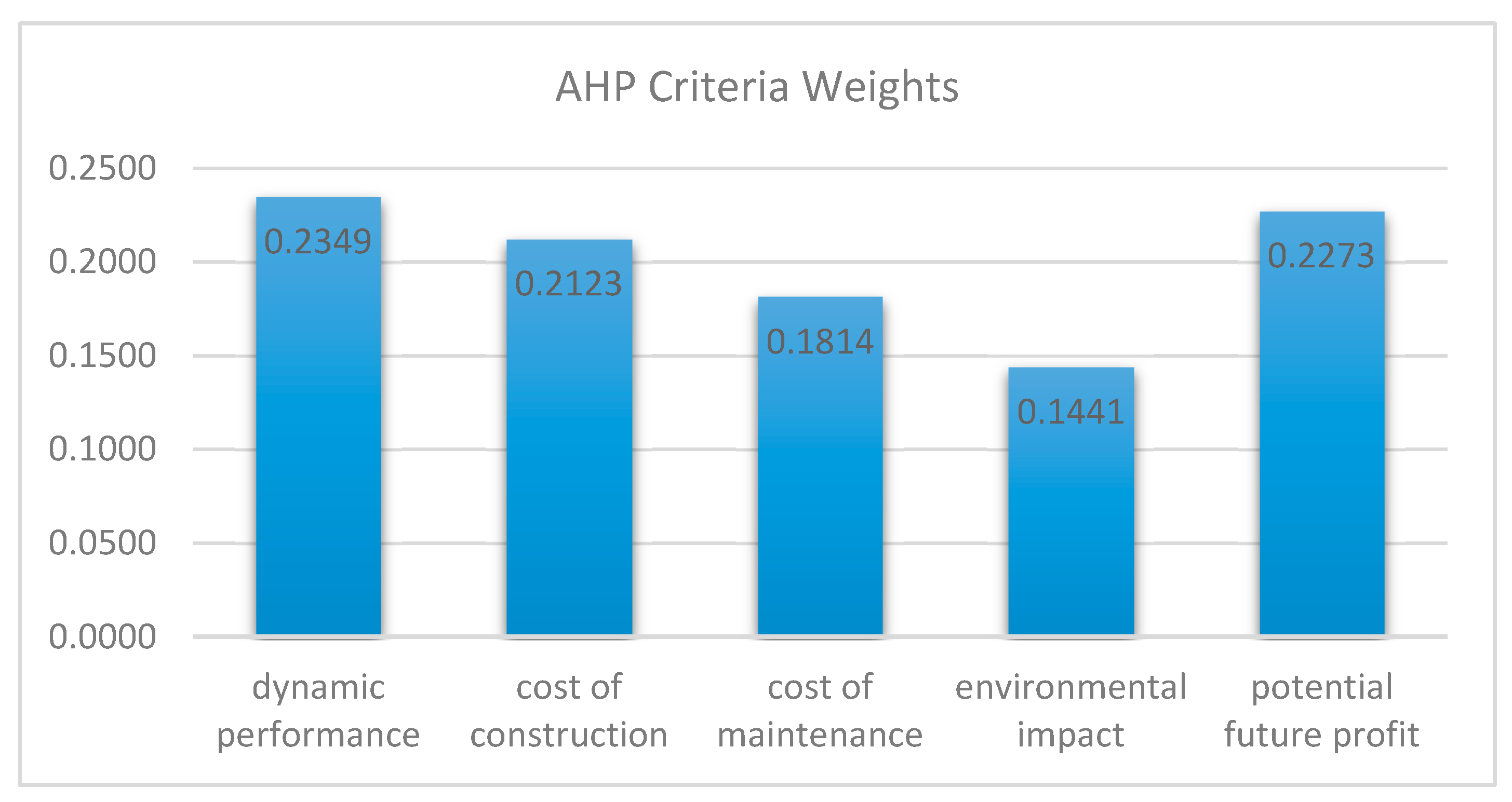
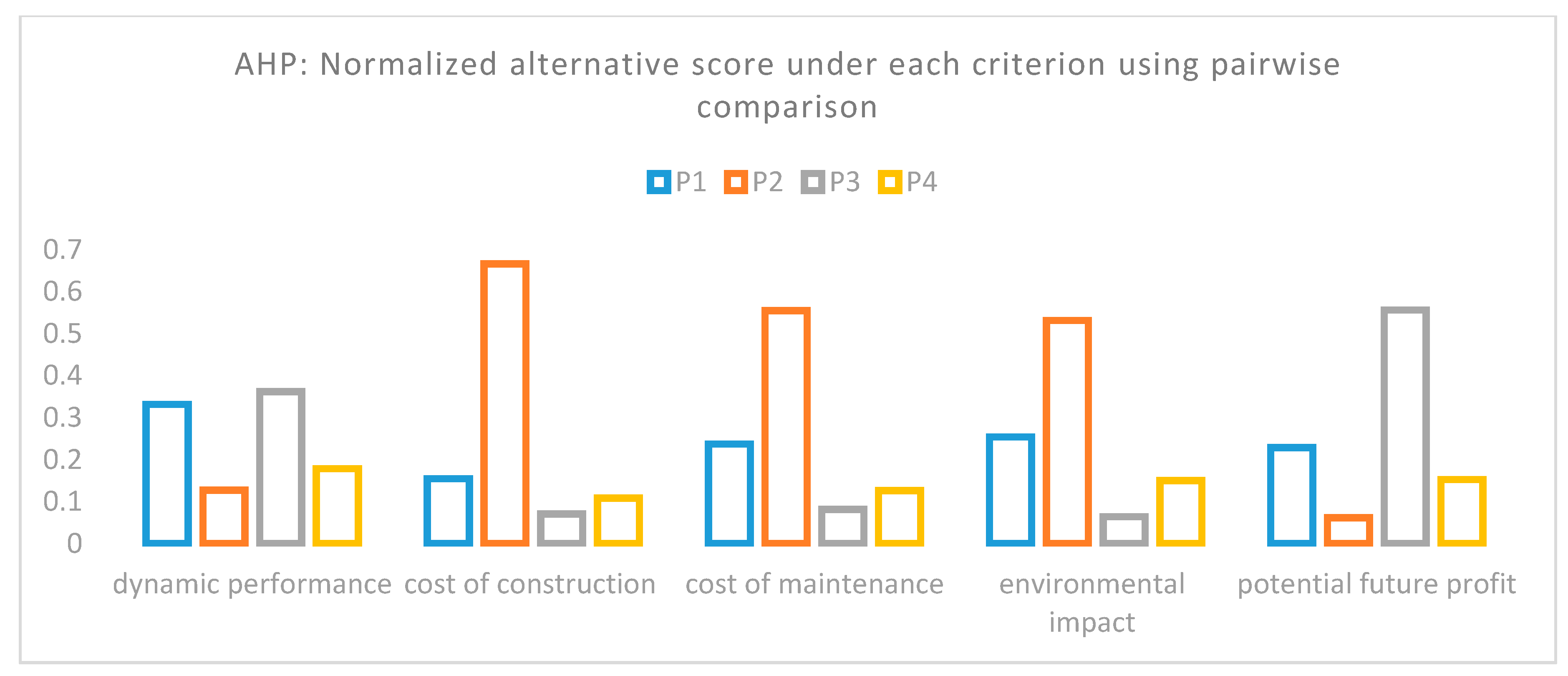
Figure 7 shows the criteria weight resulting from using pairwise comparison. Dynamic performance has the highest weight, followed by potential future profit and cost of construction. Environmental impact and the cost of maintenance have the lowest weights. All the professionals are comfortable with the weight distribution among the criteria. Figure 8 displays the alternatives’ performance for each criterion. P3 and P1 are the top two in terms of dynamic performance, followed by P4, which is less than half of P3, and P2 is the lowest of all. Regarding the cost of construction, the cost of maintenance and environmental impact criteria, the alternatives have relatively similar normalized score behavior, where the least expensive project (P2) clearly outperforms the other alternatives, while P3, the most expensive project, has the lowest score, and P1 and P4 are in the middle. For potential future profit, P3 has the highest score—almost three times more than the runner up, P1. P4 is in third position, which is less than half of P1 and two times higher than the last one, P2.

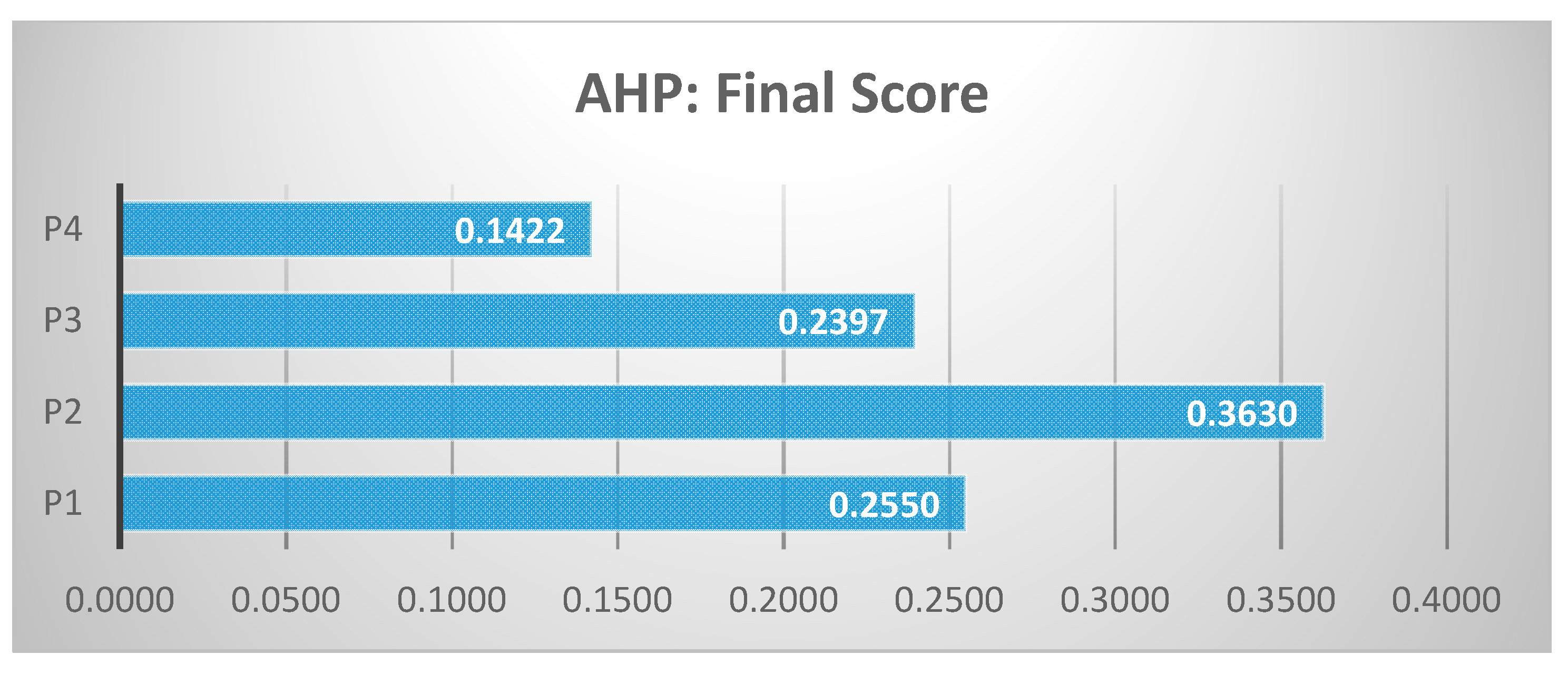
The results from Figure 7 and Figure 8 summarize the final score and derive the rank of the alternatives, shown in Figure 9, where P2 is the optimal alternative according to the AHP methodology, followed by P3 and P1. P4 receives the lowest score.

3.2.2. TOPSIS

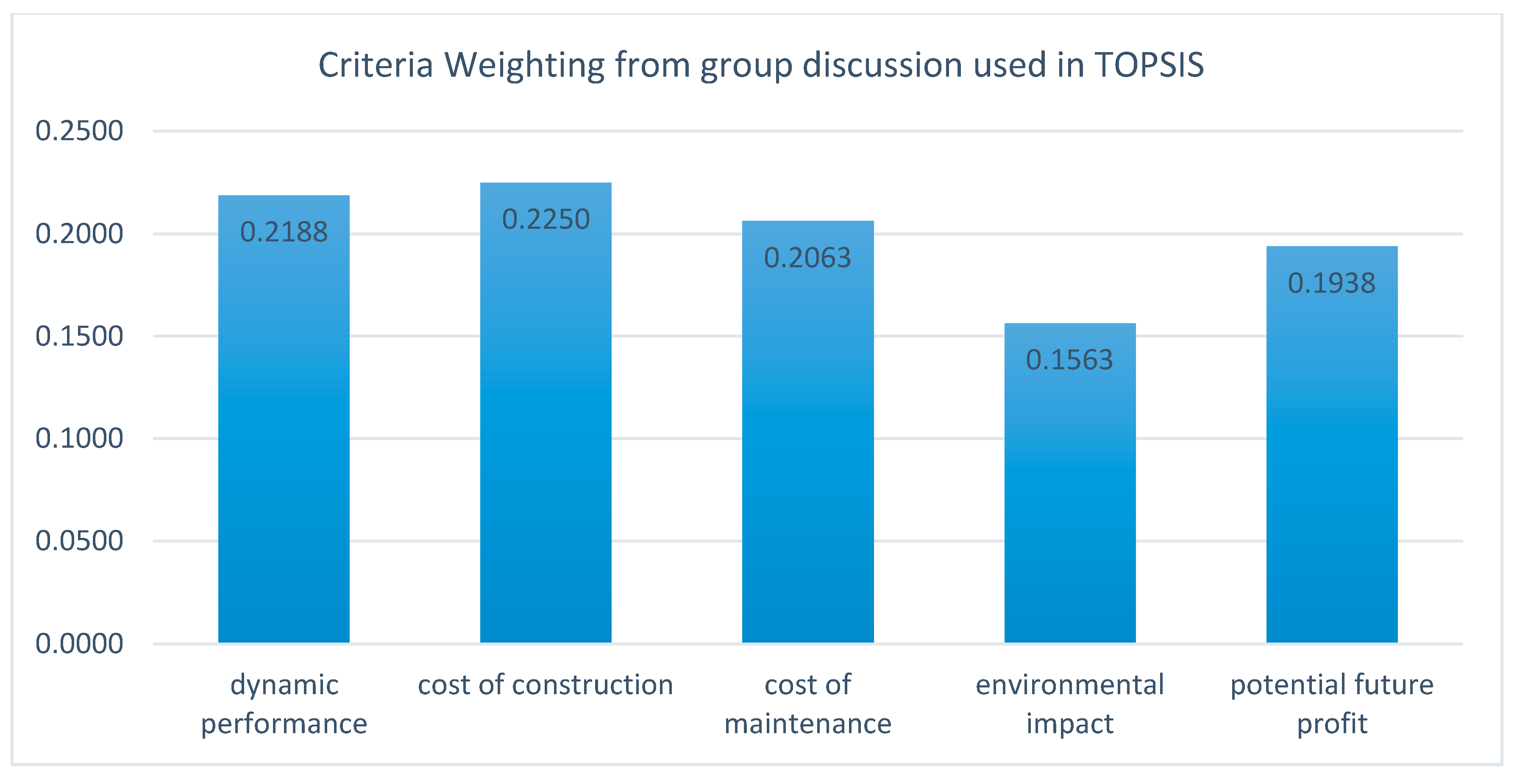
When implementing the TOPSIS process, each professional can assign criteria weighting based on his/her own knowledge. Professionals choose a value between 0% and 100%; the higher the percentage, the greater the criterion’s weighting. For simplicity, the total sum of the assigned weighting of the five criteria must equal 100%. With three rounds of the Delphi technique, each professional finalized his/her assignment, and the final criteria weighting is calculated by taking the average from all professionals; the result is shown in Figure 10. The weighting is almost equally distributed among dynamic performance, cost of construction, cost of maintenance and potential future profit, while environmental impact received a lower weighting.

After deciding the criteria weighting, the TOPSIS process also requires all professionals to provide their opinions on the alternatives’ performance for each criterion in order to form the decision matrix. Furthermore, due to the normalization in TOPSIS, the alternatives’ performance for different criteria must be expressed in the same measurement unit. Hence, in order to formalize their opinion, all professionals are asked to rate the alternative between 1 and 10 for each criterion, where 1 denotes extremely poor performance and 10 denotes excellent performance. For example, P1 is rated by each expert (columns in

Table 6. Professionals’ ratings for P1.

P1	Project Manager	Civil Engineer 1	Civil Engineer 2	Road Operator 1	Road Operator 2	Wea&Env Expert	Sanitary Engineer 1	Sanitary Engineer 2	Average
Dynamic performance	8	8	8	7	7	7	7	7	7.375
Cost of construction	6	6	6	7	6	6	6	6	6.125
Cost of maintenance	7	7	6	6	6	6	6	6	6.25
Environmental impact	7	7	7	7	7	6	7	7	6.875
Potential future profit	7	7	8	8	8	7	7	7	7.375

) for each criterion (rows in Table 6), and P1′s final rating for one criterion is the average of all the professionals’ scores. The final column “Average” in Table 6 is the final score for P1 for different criteria. Note that the scores in Table 6 are from each expert and are also derived through the Delphi technique.

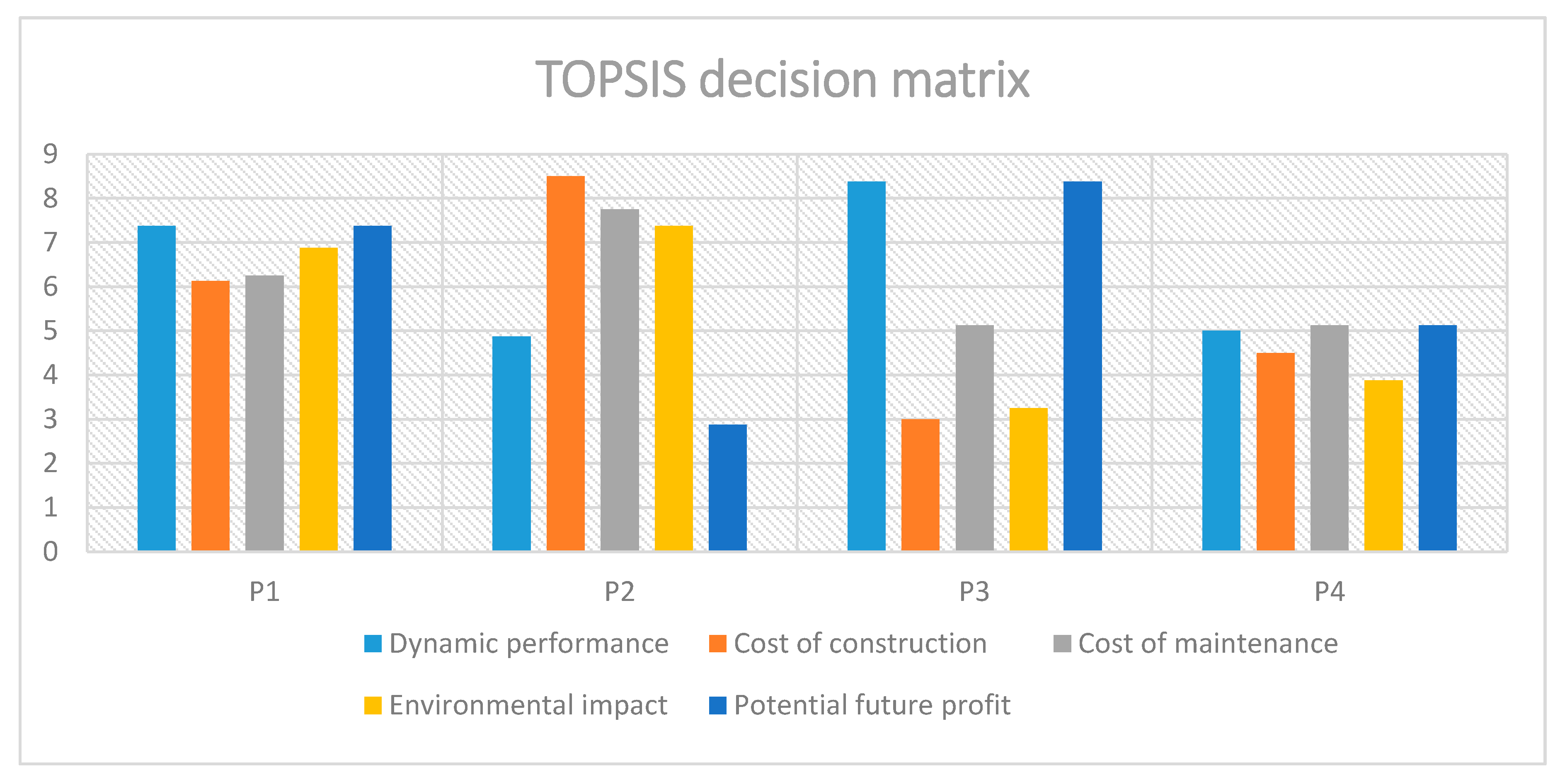
This process is repeated for all the other alternatives, and the decision matrix is formed by the average rate of each alternative for each criterion; see

Table 7. TOPSIS: Decision matrix for case study.

Alternatives Criteria	P1	P2	P3	P4
Dynamic performance	7.375	4.875	8.375	5
Cost of construction	6.125	8.5	3	4.5
Cost of maintenance	6.25	7.75	5.125	5.125
Environmental impact	6.875	7.375	3.25	3.875
Potential future profit	7.375	2.875	8.375	5.125

. Figure 11 illustrates the decision matrix for Table 7 for a better overview. P1 received above 6 for all the criteria. P2 has a very good rate (over 8) in terms of cost of construction, which is reasonable since its construction cost is significantly lower than the others. P3 has very good rates for the dynamic performance and potential future profit criteria (both are over 8), while it does not have any advantages for cost of construction and environmental impact. P4 receives relatively similar rates for all criteria and the average is 4.5.

After the decision matrix is built, the next steps in TOPSIS are: deriving the standardized matrix; next, considering the weights of the criteria to get the weighted standardized matrix; followed by finding the ideal solution $S^{+}$ and anti-ideal solution $S^{-}$ in order to calculate the Euclidean distance from each alternative to the ideal solution $S^{+}$ and the anti-ideal solution $S^{-}$, i.e., $D_i^{+}$ and $D_j^{-}$; finally, obtaining the relative closeness. The optimal choice is the one with the highest relative closeness value.

Table 8. TOPSIS. Results for sewer network planning case study.

TOPSIS Results	P1	P2	P3	P4
Rank	1st	2nd	3rd	4th
Relative closeness	0.6663	0.5538	0.4462	0.2672

shows the result from TOPSIS, where P1 receives the highest relative closeness value, i.e., it is the alternative that is the farthest from the anti-ideal solution and nearest to the ideal solution.

3.2.3. ELECTRE III

The ChemDecide decision framework is introduced and developed in Hodgett (2016), where Hodgett explains the workflow for ELECTRE III and illustrates how to use the software by applying it to an equipment selection decision problem.

The ChemDecide framework contains four different tools, one related to structuring the decision-making problem and the other three associated with the analysis provided by three different MCDM methodologies—one of the methodologies is ELECTRE III. The problem-structuring tool requires the user to designate a goal, a set of alternatives and a defined set of criteria (including whether the criterion is qualitative or quantitative and minimizing or maximizing). The analysis tool requires the decision-maker to input the criteria weights and the alternatives’ performances.

It is time consuming and unrealistic to ask each expert to use the software. Since all experts have attended several group meetings to structure the decision problem and to decide the criteria weights for AHP and TOPSIS, the project manager is aware of each professional’s perspective; he represents the group as the user to provide the inputs to the software. His inputs are concluded and gathered to include the perspectives of all the professionals. The complete description of this software framework can be found in Edgar Hodgett [18]. The following is a brief list of the steps in using this software to implement the sewer network planning case study.

Step 1. Choose the decision setup tool to enter the goal of the sewer network planning, all the available alternatives, plus five criteria and indicate whether each criterion is qualitative or quantitative and minimizing or maximizing.

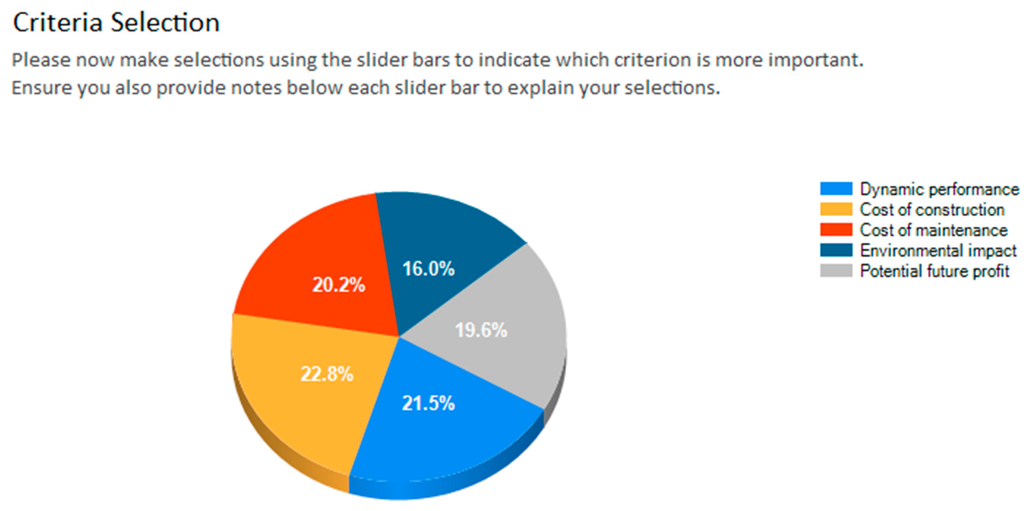
Step 2. Choose the ELECTRE III analysis tool. Open the structured problem from Step 1. Then make selections using the slider bars to indicate which criterion is more important, i.e., a higher weighting. Here, the project manager decided to use the weighting (in Figure 10) derived from the group discussion during the TOPSIS process to define the criteria weights (see Figure 12). The weights are not exactly the same because they are entered using a slider bar.

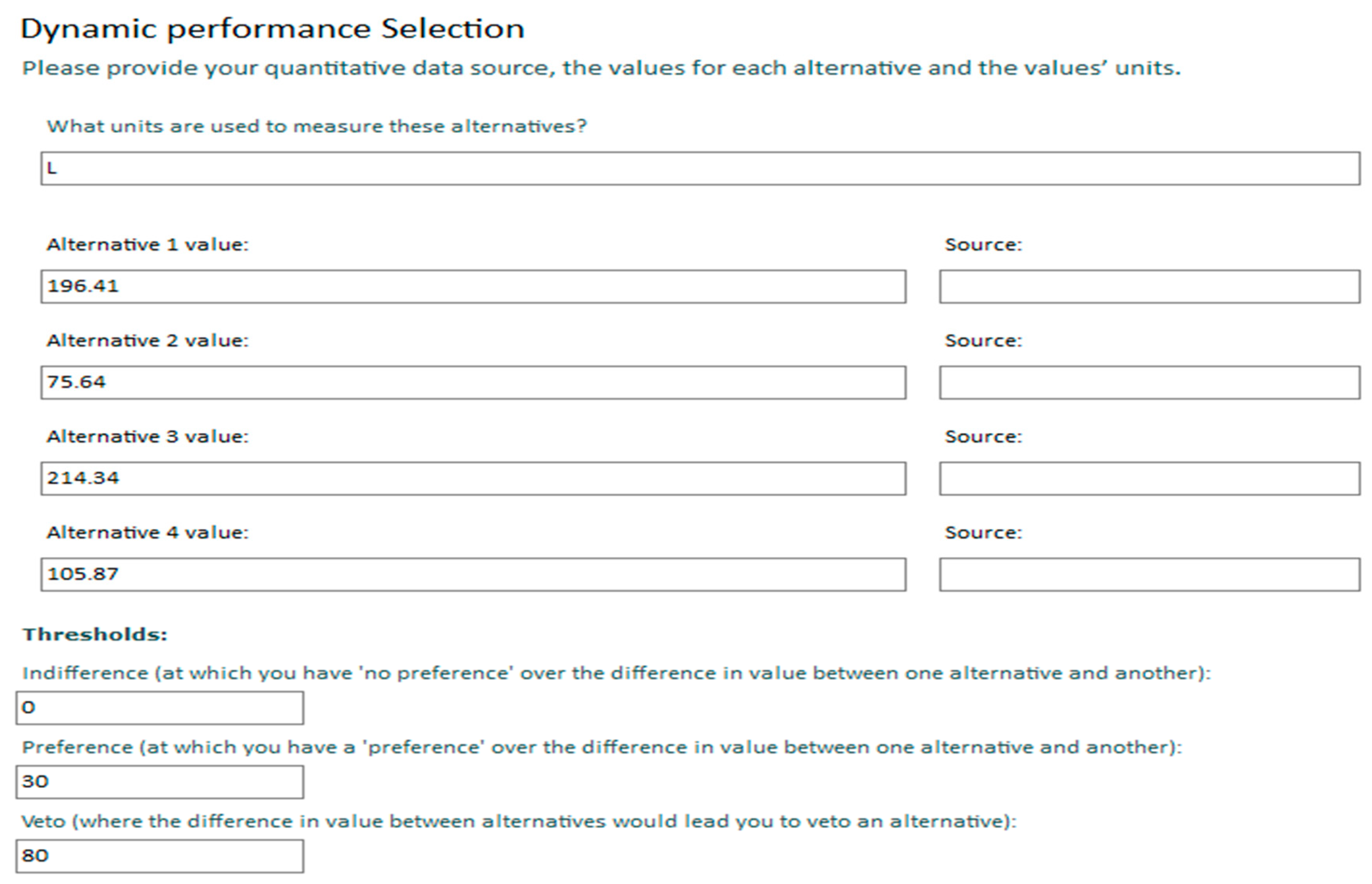
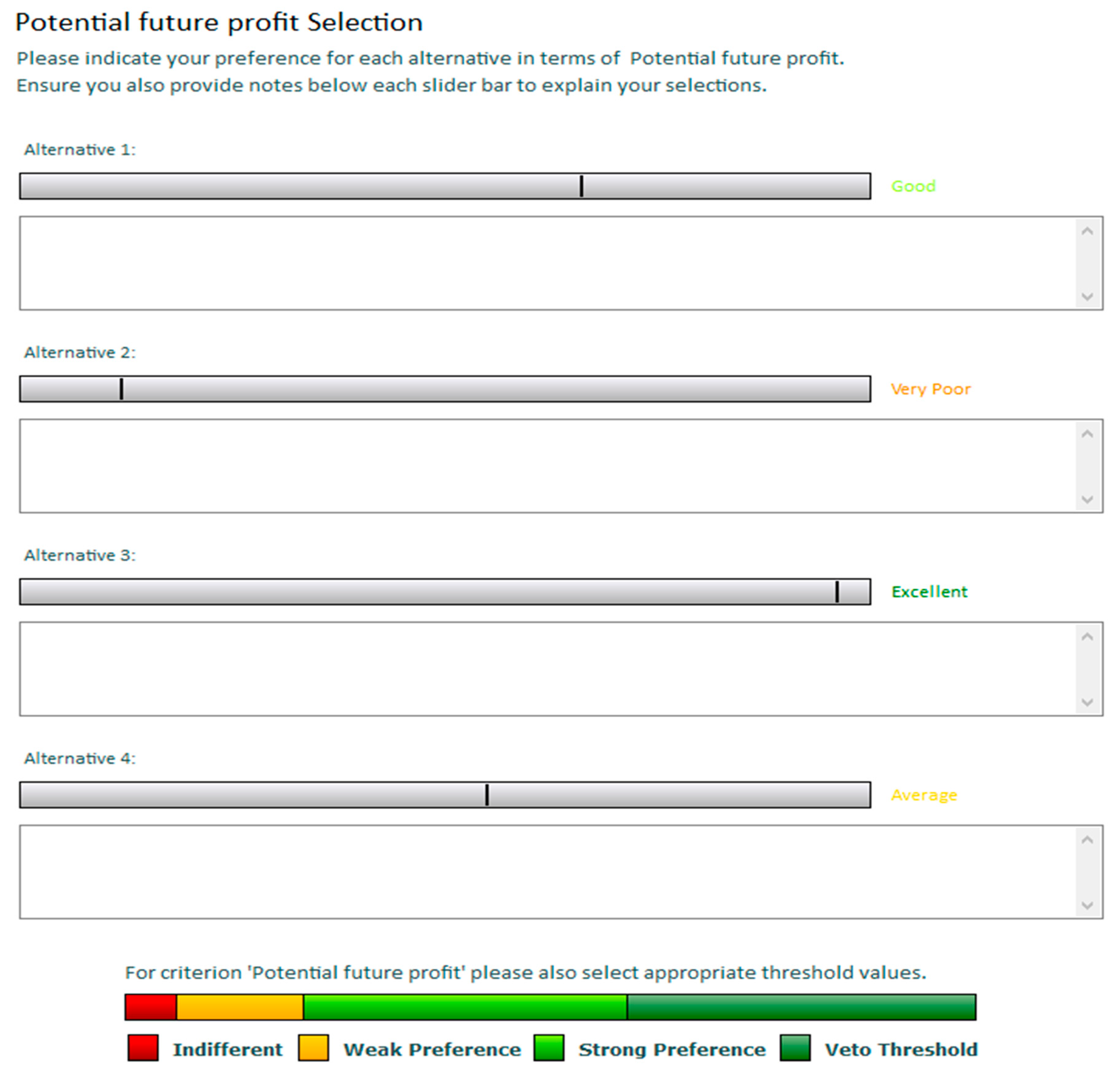
Step 3: For each quantitative criterion, enter its true quantitative data source (numerical value and unit) as well as the indifference, preference and veto thresholds. In this case, the user does not know the meaning thresholds; the tool has already provided the explanation to make sure the user entered reasonable inputs. For each qualitative criterion, the user indicates his/her preference for each alternative using the slider bar. The slider bar assigns an evaluation of extremely poor, very poor, average, good, very good, excellent. Figure 13 and Figure 14 provide some insight into the above description.

The user has entered all the information in the above steps. The software generates a report showing the results as in Table 7. It shows that ELECTRE III assigns both P1 and P2 first rank: the descending order proposes P1 as the best alternative, while the ascending order proposes P2 as the best alternative.

3.2.4. PROMETHEE II

Although all the PROMETHEE II computations can be performed manually, for the sake of simplicity, and because decision-makers can have a different experience using a manual decision-making process, a software tool is chosen to aid professionals in implementing this decision-making method.

The current available software packages for PROMETHEE are Decision Lab, D-Sight, Smart Picker Pro, and Visual Promethee [16]. From these, Smart Picker Pro [51], developed by a team from the Department of Engineering at the Free University of Brussels, is chosen. Its user-friendly interface allows decision-makers to model the decision problem step by step and enter their preferences, e.g., the criteria weighting and other preference parameters. It reflects the preference entered into the software. Also, unlike other software, it is available as a free trial version (www.smart-picker.com) with time-unlimited use. However, its trial version is limited to a maximum of five alternatives and four criteria, but this is sufficient to comprehend its application. Smart Picker Pro does not require much understanding of the PROMETHEE II method itself, which makes it very easy to use.

The algorithm behind this tool is PROMETHEE I (partial ranking) and PROMETHEE II (complete ranking). As previously mentioned, PROMETHEE II is the method used from the PROMETHEE family for this case study. Full instructions for this software can be found in [16] or the “Help” menu in the tool.

As was the case for ELECTRE III, the project manager represents the whole project group in using the software with the help of the author. The essential operating steps for the tool in solving the sewer network planning decision problem are listed below.

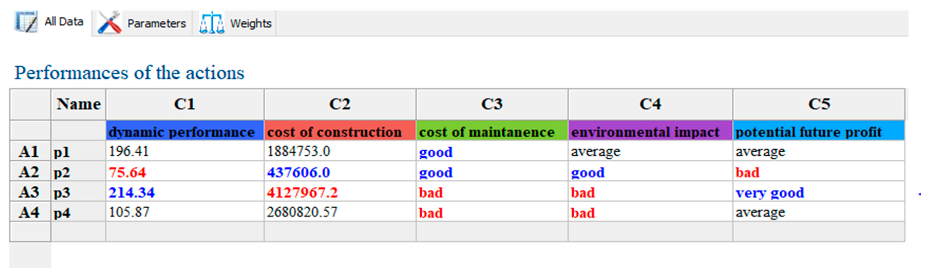
Step 1. Enter the performance of alternatives for different criteria (see Figure 12).

The performance of the alternatives for the qualitative criteria (dynamic performance and cost of construction) are based on the true experiment value, taken from Table 3 and Table 4, while the performances for quantitative criteria are evaluated on a scale of very good, good, average, bad or very bad; the corresponding scores for this scale are 4, 3, 2, 1, 0 respectively. Ultimately, both quantitative and qualitative criteria are quantified. It is worth mentioning that in the PROMETHEE method, there is no need to restrict all the performances measured to the same unit.

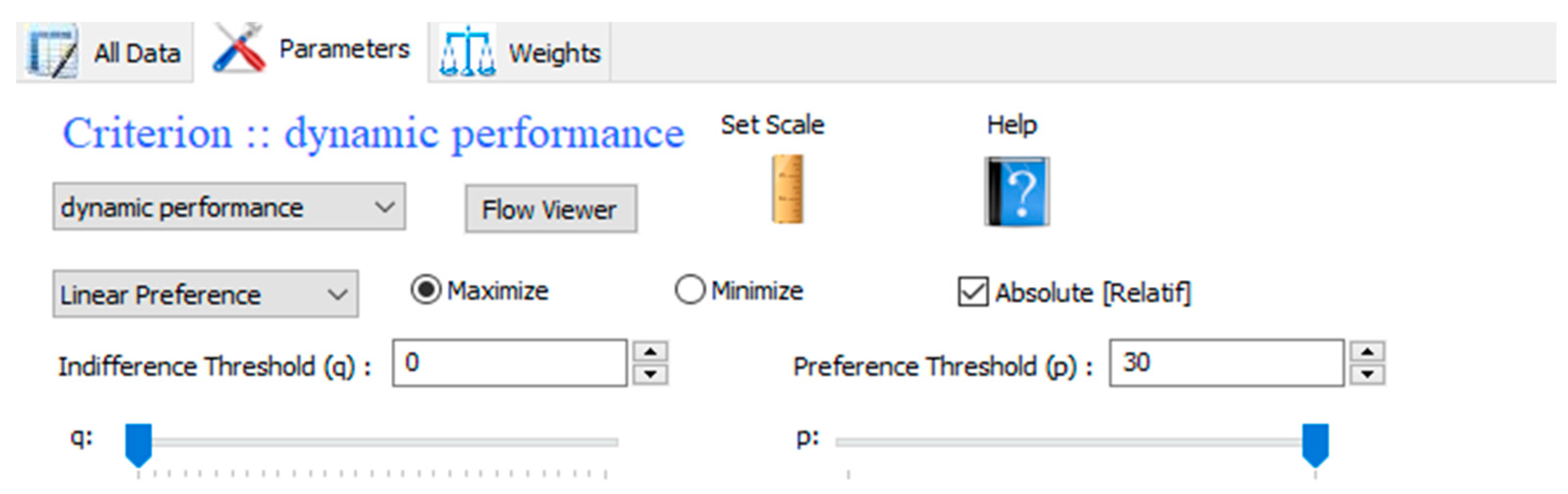
Step 2. Set up the preference parameters, such as maximize or minimize, to indicate whether the criterion is positive or negative; the preference function: the linear function is selected for all criteria; the indifference and preference threshold (see Figure 13 for the setup of one criterion).

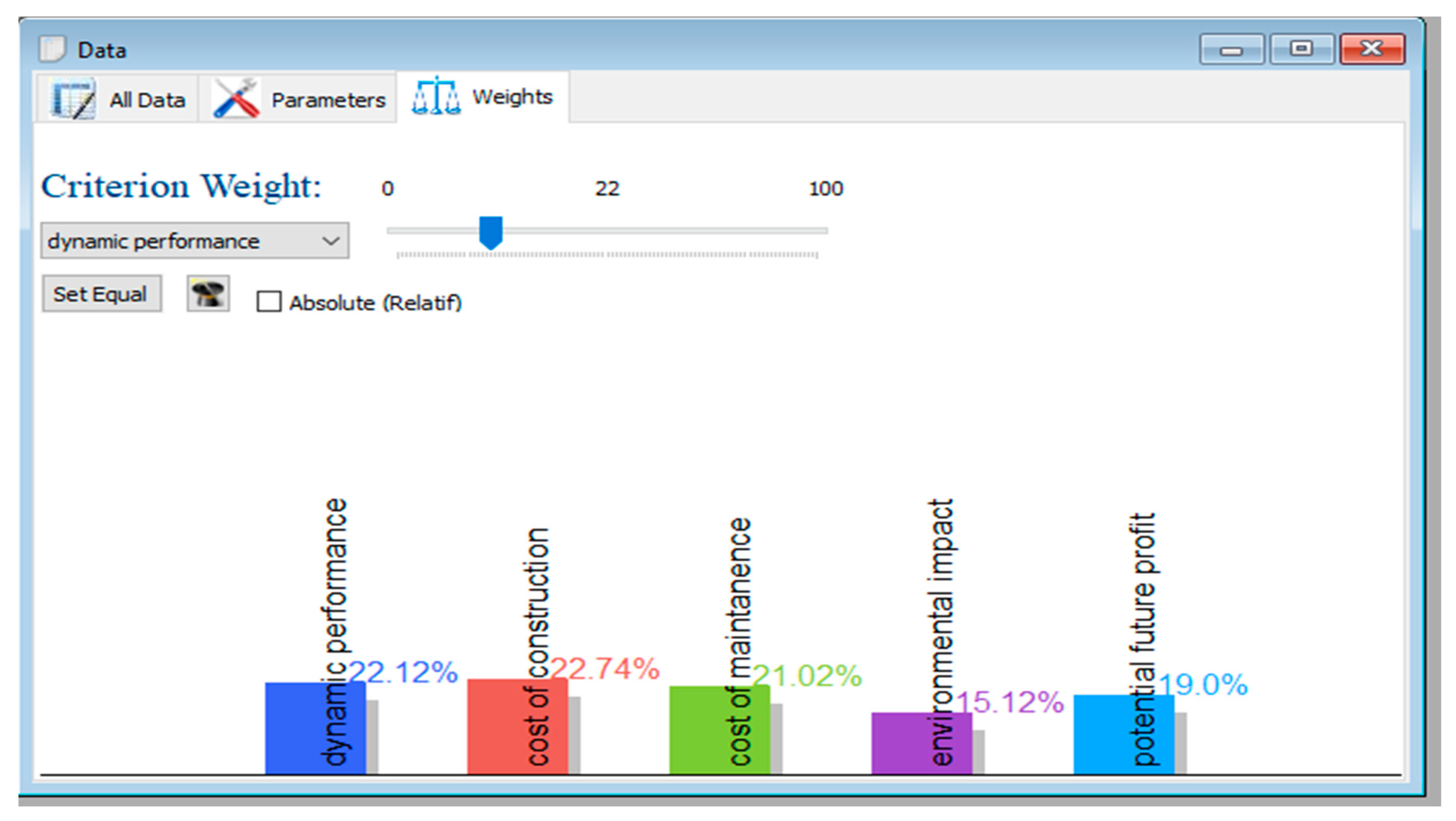
Step 3. Set the criterion weight values. In this case, the project manager decided to use the weights (in Figure 10) derived from the group discussion during the TOPSIS process. In Smart Picker Pro, users set the weights using a slider bar (see Figure 15). Note that the weights are not exactly the same values as shown in Figure 10, because the slider bar cannot provide the exact value and causes bias (see Figure 16).

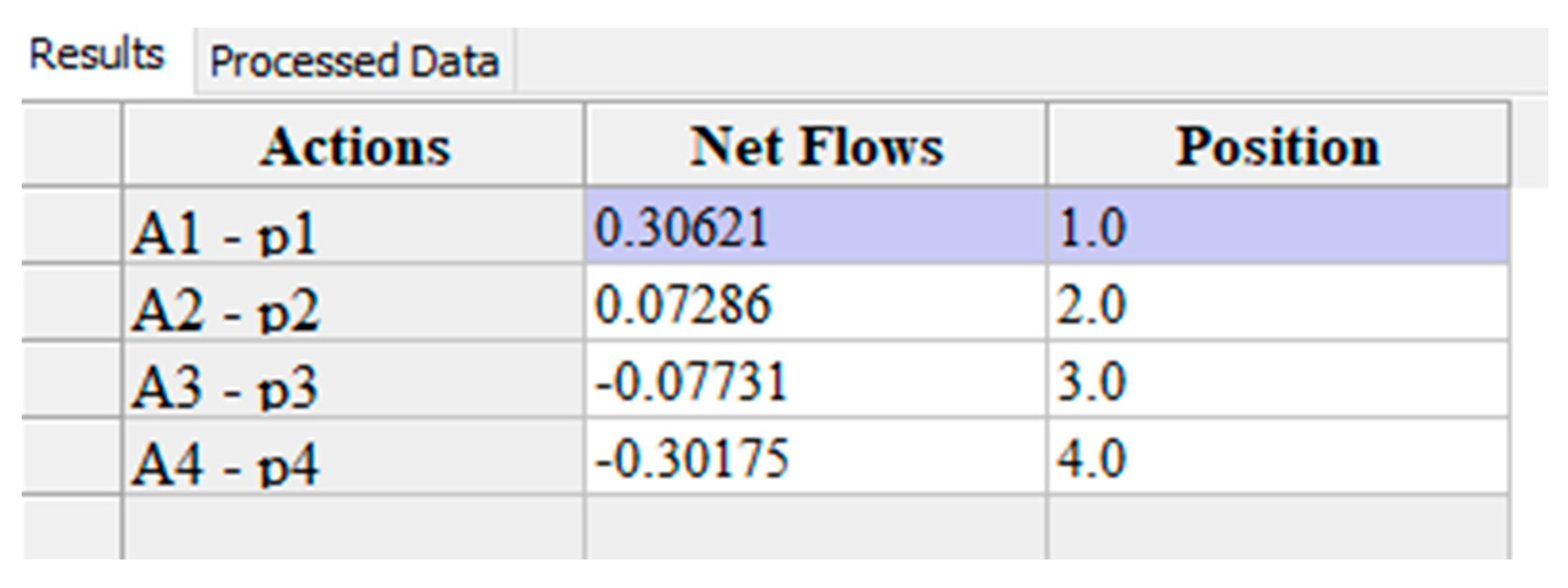
With the above steps, all the decision problem inputs are ready for Smart Picker Pro to analyze and show the final ranking result. The results are shown in Figure 17 P1, ranked in first position, has the highest net flow, which is much higher than the runner up, P2; this ensures its first position over all other alternatives. P3 and P4 received negative net flows far behind the first two.

3.3. Results Summary and Post-Analysis Interview

Figure 9, Table 8,

Table 9. ELECTRE III: result of the sewer network planning case study.

	Descending Order	Ascending Order	Final Order
First	P1	P2	P1 P2
Second	P2	P1	P3
Third	P3 P4	P3	P4
Fourth		P4

and Figure 18 show the results of AHP, TOPSIS, ELECTRE III and PROMETHEE II respectively. All of them recommend alternatives P1 and P2 over P3 and P4.

Table 10. Comparison of the four MCDM methodologies.

	1st	2nd	3rd	4th
AHP	P2	P1	P3	P4
TOPSIS	P1	P2	P3	P4
ELECTRE III	P1 P2		P3	P4
PROMETHEE II	P1	P2	P3	P4

groups all the results together. It shows that AHP chose P2 over P1 as the best option; TOPSIS and PROMETHEE II prefer P1 over P2; and ELECTRE II could not provide a conclusive decision between P1 and P2, where both are given first ranking.

The whole project team is interviewed to review their experiences and discuss the results. On reflection, for AHP, they agreed that pairwise comparison is indeed efficient and accurate in evaluating the preference between two alternatives rather than simultaneously evaluating all alternatives. However, numerous pairwise comparisons are required. Even though there is a consistency check to guarantee the subjective judgments from pairwise comparison, professionals still feel somewhat less confident with their inputs during the long pairwise comparison process. They stated that AHP is a good option for a decision involving only a few criteria and alternatives. During the TOPSIS process, experts also needed to have team meetings to decide criteria weighting and use a 1–10 scale to score the performance of each alternative for different criteria. They felt more comfortable and confident in evaluating their preference since it is less complex than pairwise comparison in terms of the number of inputs and measurement scale. This is also why the project manager used the criteria weights from TOPSIS for the other two MCDM methods instead of the weights from the pairwise comparison. They also wanted to mention that TOPSIS requires all performances for different criteria to be in the same measurement unit, even for the quantitative criteria, which means their true experimental values cannot be input into the decision matrix, but are instead transferred to a 1–10 scale. This also causes bias for the final score. The two software tools for ELECTRE III and PROMETHEE II are easy to operate and understand, which is the opposite of their complex underlying algorithms. The project manager found that the whole experience with software tools for the decision-making process was positive in terms of organization. It helped him to have a clear structure of the decision problem and give all necessary and correct inputs. Moreover, he had a clear view of the relations between the input values and the outcomes so that he is aware of which factors had more impact during the process. Therefore, using software tools reduced the disadvantages of these two methods. The result from PROMETHEE II is clearly indicated via each alternative’s net flow value, while ELECTRE III does not give a specific score to each alternative. Besides, ELECTRE III could not make a definite decision between P1 and P2, which made it more clear from the decision-maker’s point of view.

3.4. Comparative Analysis and Discussion

In order to fully understand the decisions reached by different MCDM methods, a deep comparative analysis is carried out on two factors: criteria weights obtained during the different MCDM processes and alternatives’ scores for each criterion assigned by different methods.

3.4.1. Comparison of Criteria Weights

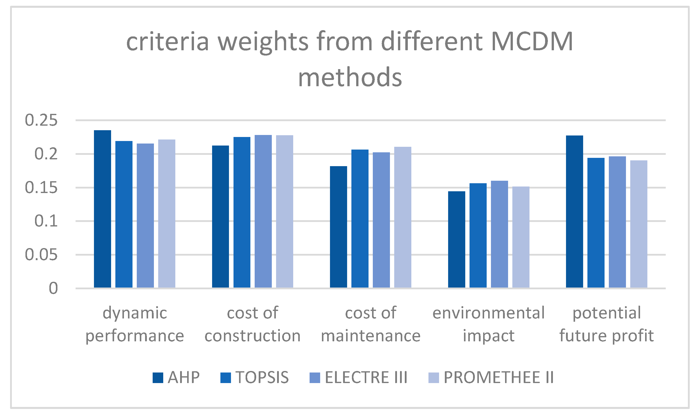
In Figure 19, each criterion’s weights derived from AHP, TOPSIS, ELECTRE III and PROMETHEE II are displayed together for a clear picture for comparison.

In general, the weight allocations for different criteria are consistent in TOPSIS, ELECTRE III and PROMETHEE II. Inconsistency occurs during AHP, which places considerable attention on the positive criteria (dynamic performance, potential future profit) compared to the other three negative criteria.

3.4.2. Comparison of Alternative Scores

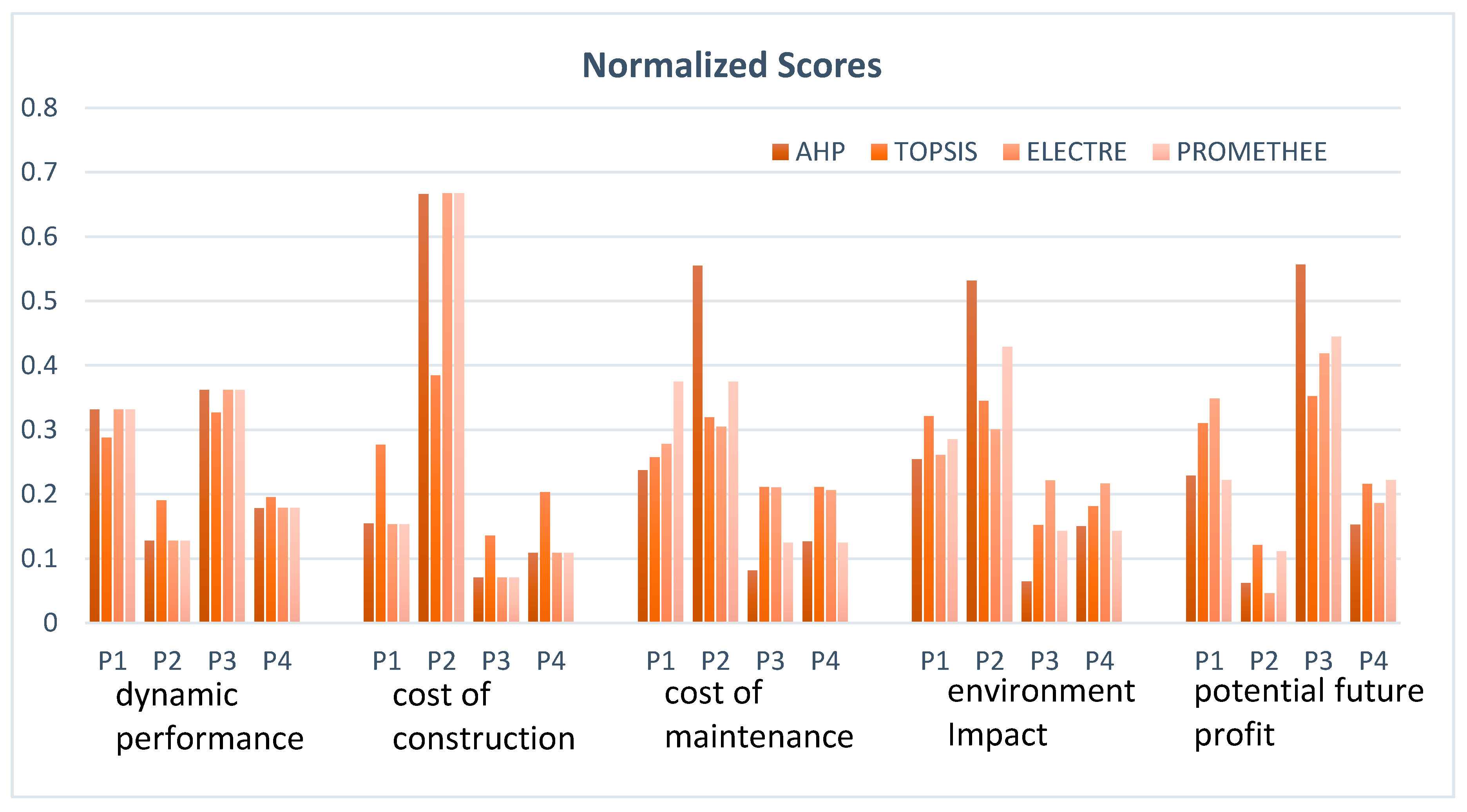
Figure 20 provides an overview of the differences for each alternative evaluated via different MCDM processes. Note that all scores have been normalized in order to make the comparison more persuasive.

For the two quantitative criteria (dynamic performance and cost of construction), the alternative scores in AHP, ELECTRE III and PROMETHEE II are consistent because the true experimental numerical values are used as input. However, in the TOPSIS process, since the decision matrix needs to be measured in the same unit, the inability to use true values for quantitative criteria causes inaccuracy.

For the other three qualitative criteria (cost of maintenance, environmental impact and potential future profit), alternative scores show a number of inconsistencies in the four MCDM methods. One explanation is that it is difficult to stay consistent when making subjective judgments on alternatives for qualitative criteria in different processes. The difficulty can be the result of decision-maker fatigue after prolonged attention and mental effort. Vohs, Baumeister, Twenge and Schmeichel [52] argue that making decision from different alternatives for various criteria requires energy, tires out decision-makers and thereby impairs self-regulation. Vohs, Baumeister, Twenge and Schmeichel [52] refer to this situation as “decision fatigue” and conclude that “self-regulation was poorer among those who had made choices than among those who had not.” Another explanation for the inconsistency is that decision-makers might feel that the impact of scores for qualitative criteria are minor. However, to have a sound, reliable decision result from a structured decision analysis requires decision-makers to express their preferences more carefully.

Nevertheless, it is worth mentioning that AHP has the most inconsistencies for qualitative criteria, with the majority of scores showing higher or lower criteria weights than the other three MCDM methods. This situation is in line with the criteria weights from AHP discussed in Section 3.4.1. This happened even though all of the decision-makers’ pairwise comparisons are theoretically consistent, i.e., the consistency ratio is less than 0.1. Therefore, either the decision-makers placed emphasis on their preferences on purpose or there are inaccuracies in the 1–9 fundamental scale proposed by Saaty and Vargas [23]. In fact, Salo and Hamalainen [53] point out that there is an uneven dispersion of values in Saaty’s AHP selection scale. They conclude that the difference in selecting between the scale of 1 and 2 is 15 times greater than the difference in selecting between the scale of 8 and 9. This indicates that Saaty’s AHP selection scale is responsible for the overemphasized criteria weights and alternative scores in the case study.

4. Conclusions and Future Work

Making a decision on a sewer network construction project is important for urban development, public health and environmental sustainability. It has been suggested that a group of decision-makers should apply an effective and efficient MCDM method for the sewer network decision problem. However, different methods have their own limitations, hypotheses, premises and perspectives, which leads to different decision results when applied to an identical problem. This paper provides a comparative study on four different MCDM methods (AHP, TOPSIS, ELECTRE III and PROMETHEE II) from their distinctive theoretical algorithms and from their implementation on one sewer network planning group decision problem. AHP and TOPSIS were implemented via spreadsheets, while ELECTRE III and PROMETHEE II were applied via available software tools due to their complex algorithms. A number of conclusions can be drawn:

• Five criteria require ten pairwise comparisons to determine the criteria weights in AHP, which is more time consuming. The other three methods only need ten inputs. By increasing the number of criteria and alternatives, AHP is not a practical method to implement.
• The criteria weights and scores of the four methods are inconsistent, with AHP showing the greatest variation (Figure 19 and Figure 20). This is most likely because of inaccuracies with AHP’s 1–9 fundamental scale, decision fatigue and decision-makers’ perception that qualitative criteria with low weights have minor impact on the decision results.
• There are visible differences in the results of the four methods (Table 10). It needs to be pointed out that ELECTRE III was unable to provide a conclusive result, identifying both P1 and P2 as the best alternatives. PROMETHEE II and TOPSIS prefer P1, while AHP selects P2 as the best option. In general, P2 receives extremely high scores on three criteria and extremely low scores on the other two criteria, while P1 has a more or less average evaluation on different criteria. When considering this, decision-makers all prefer P1 over P2.
• TOPSIS requires all the performances for different criteria to be expressed in the same measurement unit. This makes decision-makers feel that TOPSIS is limited when the true numerical experimental values cannot be used as input directly.
• PROMETHEE is the favored method for decision-makers in terms of the decisive result identifying P1 as the best option and decision-makers’ satisfaction with the implementation process.

The comparison of the different MCDM methods directly helped the whole project team to make an informed decision. By going through this process, all the experts became more knowledgeable about their decision and the uncertainty associated with each sewer network plan. The results clearly show that there is a risk in following the results of one particular MCDM method. Therefore, if time permits, it is advisable to approach a sewer network group decision problem using different decision-making methods. However, if time is a limitation then the results indicate that PROMETHEE II is the method that most effectively provided an accurate representation of the decision-makers’ preferences. The conclusion of this paper should also encourage industry professionals to cooperate with academic researchers in order to examine the compatibility of a wider range of MCDM methods with sewer water infrastructure management. More case studies are required to test and validate the theories, since the recommendations presented in this paper are based on only one sewer network decision problem.