Article

Micro-Mechanical Hyperelastic Modelling for (Un)Filled Polyurethane with Considerations of Strain Amplification

1
Fraunhofer Institute for Manufacturing Technology and Advanced Materials IFAM, D-28359 Bremen, Germany
2
Faculty 4—Production Engineering, University of Bremen, D-28359 Bremen, Germany
*
Author to whom correspondence should be addressed.
Modelling 2024, 5(2), 502-529; https://doi.org/10.3390/modelling5020027
Submission received: 8 March 2024 / Revised: 12 April 2024 / Accepted: 18 April 2024 / Published: 24 April 2024

Abstract

:
Polyurethane (PU) is a very versatile material in engineering applications, whose mechanical properties can be tailored by the introduction of active fillers. The current research aims to (i) investigate the effect of active fillers with varying filler loads on the mechanical properties of a PU system and (ii) develop a micro-mechanical model to describe the hyperelastic behavior of (un)filled PU. Three models are taken into consideration: without strain amplification, with constant strain amplification, and with a deformation-dependent strain amplification. The measured uniaxial stress–strain data of the filled PU nanocomposites reveal clear reinforcement due to the incorporation of carbon black at 5, 10 and 20 wt%. In low concentration (1 wt%), for two different grades of carbon black and a fumed silica, it results in a reduction in the mechanical properties. The micro-mechanical model without strain amplification has a good agreement with the measured stress–strain curves at low concentrations of fillers (1 wt%). For higher filled concentrations (5–15 wt%), the micro-mechanical model with constant strain amplification leads to a better prediction performance. For samples with a larger filler volume fraction (20 wt%) and for a commercial adhesive, the model with a deformation-dependent strain amplification effect leads to the best predictions, i.e., highest R2 regarding curve fitting.

1. Introduction

Due to the favorable stress state in bonded joints, adhesive bonding technology is favored for joining thin-walled lightweight structures [1]. The adhesives are used in (multi-material) bonding on coated metal and on fiber-reinforced composites (FRP) in automotive engineering, aerospace technology, shipbuilding, rail vehicle construction, and the electrical industry. The long-term durability of the bonded joints is decisive for an economically reasonable use of the joining technology [2]. With the increasing use of FRP in the automotive industry, hyperelastic polyurethane (PU) adhesives, which are very suitable for structural applications, are increasingly gaining in importance [3,4].
Efficient characterization of the mechanical properties of PU adhesives can hardly be achieved without the help of numerical methods [5]. The finite element method (FEM) has developed into an indispensable tool for computer-aided simulation and stress analysis of complex components which can be carried out within a reasonable timeframe [6]. It should be noticed that nonlinear stress–strain behavior is a key characteristic of PU adhesives [7]. It follows that this nonlinearity must be taken into account in the numerical prediction of adhesive bonds, particularly when they are subjected to large deformations. The description of such complex material behavior in FEM is carried out with the help of hyperelastic material models. These models provide a relationship between the deformation and the resulting stress for a given temperature and loading rate. Hyperelastic material models can be divided into two main groups: phenomenological and micromechanical models [8].
The phenomenological models are based on the macromechanics of deformation and are hence not concerned with the microscopic nature of the material. A well-known representative of this group is the Mooney–Rivlin model [9,10]. The micromechanical models on the other hand are derived from the deformation kinetics of the polymer chain in the network. One can mention the eight-chain model developed by Arruda and Boyce [11] as a well-known example of a micromechanical approach.
With the increasing number of considered influence parameters, the experimental effort for parameter identification increases extremely with a purely phenomenological approach. The usual testing of adhesive samples leads to an unmanageable amount of samples and parameter diversity for phenomenological models. Long-term tests are very cost-intensive and time-consuming. Hence, the development of physically motivated material models can be of great economic importance to limit the experimental effort for parameter identification to an acceptable scope from an industrial point of view.
In the micromechanical model, in contrast to the phenomenological approach, the physics of the polymer network is considered. From the point of view of the statistical mechanics, the network consists of interaction-free individual polymer chains located between crosslinks. The entropy change of the chain when it is stretched and the corresponding restoring force can be calculated using statistical evaluation (entropy elasticity) [12]. The elastic response of the polymer network is usually calculated as the average value of the elasticity of the single chain averaged over all possible orientations [13]. Due to the numerical effort of this averaging, models have been developed in various works [14,15] that deal with discrete chains in a unit cell.
To improve mechanical properties and to reduce the manufacturing costs, active (reinforcing) fillers are added to the PU matrix of the engineering materials. Such fillers mainly comprise aggregates of nanoscale particles exhibiting a higher stiffness compared to the polymer matrix [16]. Silica and carbon black could be named as classical representatives of this group of fillers [17]. Therefore, most PU adhesives can be considered as filled materials. However, there is not a universal modelling approach with regard to the filler effect on mechanical properties of PU. Moreover, in a number of publications, at some filler concentration regimes, a deterioration of some mechanical properties is reported, whereas for most concentrations, the obtained results exhibit a clear reinforcement of the PU elastomers brought about by active fillers [18,19].
PU elastomers present a microphase-separated morphology. The hard phase, i.e., the hard domains, being rigid and glassy in nature, do not solely provide connectivity between network strands. They also impart reinforcement to the material [20]. One may consider a polyurethane network as a particulate composite material where hard domains are uniformly dispersed in a rubbery matrix representing the soft phase. In order to account for the reinforcement effect of the hard domains, one focus can be directed towards the strain amplification concept according to Mullins and Tobin [21,22].
The strain amplification assumes that incorporation of filler leads to a consequent distortion of the stress pattern within the PU matrix. Thus, the matrix is prevented from deforming uniformly by polymer–filler adhesion, which, in turn, makes the overall apparent strain less than the strains occurring locally. Consequently, the ratio of the stress to strain is increased by a factor of X [21,22].
Within this background, the aim of the current research is twofold: (i) investigate the effect of active fillers with varying filler loads on the quasi-static uniaxial properties of a pure PU model system, and, (ii) develop a micro-mechanical model able to describe the hyperelastic behavior of filled PU systems with consideration of strain amplification.

2. Materials and Methods

2.1. Sample Material

To investigate the effect of active fillers on the mechanical properties of PU, composites were prepared for uniaxial tensile tests. For this purpose, PU-nanocomposites were prepared using a commercially available elastomeric casting resin, with the trademark Sika Biresin® U1404 (Sika Deutschland, Rosendahl, Germany), which is based on toluene diisocyanate (2,4-TDI) and poly (propylene) glycol (PPG). The so-called component A of the PU is an aromatic pre-polymer produced by the reaction between toluene diisocyanate (TDI) and polypropylene glycol or polypropylene oxide. The latter is a high-molecular-weight polyether also known as PPG. The B component (hardener) of the PU system is a low-molecular-weight aromatic diamine known as diethyl toluene diamine (DETDA). The mixing ratio A:B in parts by weight is 80:100 corresponding to the shore hardness A 40.
The filled samples contain a furnace carbon black, namely Printex® 30 (manufactured by Orion Engineer Carbons, Hanau, Germany), in different weight fractions (percentage by weight, abbr. wt%) up to 20%. Also prepared are PU-nanocomposites comprising 1% Special black 250 (a furnace carbon black from Orion Engineer Carbons), and 1% Aerosil® 200 (a fumed silica produced by Evonik, Essen, Germany). The weight fraction represents the mass of the filler with respect to the total mass of the sample.
As shown by SEM images in Figure 1, Special Black 250 exhibits coarser particles of average size around 47 nm, whereas Printex® 30 consists of smaller particles with a size around 27 nm. These particle sizes correspond to special surface areas 48 and 80 m2/g, respectively. Another key difference between these two carbon blacks is their structure, whose measure is the DBP or oil adsorption number. It should be mentioned that all three fillers are provided in powder form, the reason being that, compared with beads, powders are easier to disperse.
In comparison to Special Black 250 with a DBP number of 45 mL/100 g, Printex® 30 exhibits more openly structured aggregates, i.e., aggregates with a larger void volume, reflected by a DBP number of 108 mL/100 g. Among the three fillers used for the sample preparation, Aerosil® 200 has the smallest average particle size, namely 12 nm according to supplier information. Although the DBP number is not explicitly provided by the manufacturer, Aerosil® 200 exhibits a considerably large structure implying aggregates and agglomerates that are predominantly chain-like and branched. Due to these mentioned properties of Aerosil® 200, its processability is quite poor which makes the dispersion at a large filler concentration very challenging. Such a poor dispersion results in flocculation or sedimentation of the filler which finally has a negative impact on the mechanical properties of cured samples.
The filler structure is another factor affecting the quality of dispersion. Dispersion of fillers with low structure requires more effort. In the first step of dispersion, the filler must be optimally wetted by the polymer. However, a low structure, such as that of Special Black 250, implies that optimal penetration of the polymer into the void space of filler aggregates cannot take place. This makes the wetting of the filler by the matrix more difficult. In addition, primary particles in the aggregates of a low-structured filler are more densely packed. As a result, in order to break up large agglomerates into smaller units, a larger number of inter-aggregate contacts must be overcome. Hence, similar to the case of Aerosil® 200, obtaining an optimal dispersion of Special Black 250 is also a difficult task.
Due to the above-mentioned difficulties regarding the dispersibility of Aerosil® 200 and Special Black 250, Printex® 30 is used as the main filler material in the preparation of PU composites. Nevertheless, samples including a small amount (1 wt%) of Aerosil® 200 and Special Black 250 are as well prepared to have at least one comparative case for the effect of the three individual fillers on the mechanical properties of PU.
For the validation of micro-mechanical models, a one-component commercial adhesive produced by Sika Deutschland (Rosendahl, Germany), the Sikaflex®-250 UHM, is employed.
The corresponding volume fractions ϕ , the ratio of the filler volume to the total volume of the sample, are obtained using the elementary formula ϕ = w ρ m / [ ρ f 1 w + ρ m w ] and are given in Table 1. In this relation, the weight fraction of the filler is indicated by w , while ρ m = 1.05   g / c m 3 and ρ f 1.9   g / c m 3 are the mass density of the polymer matrix and the carbon black, respectively. In the case of Aerosil® 200, we have ρ f = 2.2   g / c m 3 .

2.2. Sample Preparation

In the sample preparation process, the filler is first added to component B of the PU system. This is due to the lower viscosity of the hardener in comparison to the pre-polymer which makes the dispersion of the filler easier. The two ingredients are then mixed in a speed mixer for two minutes.
The next step is the dispersing process which plays a decisive role in obtaining the desired mechanical properties of the final product. The main goal of dispersion is to optimize the wetting of the filler by the polymer, and to break up large agglomerates through shear forces and hence to have a homogeneous particle distribution in the matrix. For this purpose, a three-roller mill is employed. As shown in Figure 2, it consists of three cylinders whose rotational speeds and the distance between them can be adjusted.
The friction between the rotating rollers and the paste generates high shear forces necessary for the separation and reduced size of the filler agglomerates. The three-roller mill is mainly used for the samples filled with 5, 10, 15, and 20 wt% Printex® 30, as this dispersion equipment is mostly suitable for highly viscose media. For samples filled with 1 wt% filler, a conventional dissolver DISPERMAT CA manufactured by VMA-GETZMANN is employed. In this dispersion method, the shear force required for the de-agglomeration is generated through a rotating dissolver disk. When dispersing with a dissolver, the optimum viscosity must be configured which mainly depends on the concentration and fineness of the filler, and the viscosity of the liquid medium. Usually, the appearance of a ring-shaped bulge (the so-called donut effect) implies an optimum viscosity for the dispersion.
Furthermore, in the sample preparation, the prepared filler–polymer slurry is heated up to 70 °C under a vacuum for 2 h to remove the possible gas bubbles formed during the dispersion process. The component A of the PU system is also heated under the same conditions. After the addition of the component A, i.e., the pre-polymer, to the slurry, the resulting mixture is blended and degassed for 4 min in a planetary centrifugal mixer under vacuum. The freshly prepared polymer–filler mixture is then carefully poured into a silicon mold, and a cannula is used to remove the gas bubbles that appeared on the surface. It should be noted that the last step should eventually be carried out more quickly, as the pot life of the PU system, around 25 min, is quite short. Lastly, the samples are cured for 5 days under room temperature.
Even after several days of curing, a residual amount of isocyanate groups might still be present in the samples. Under high-humidity conditions, the reaction of water and excess isocyanate introduces diamines, which then react to introduce urea groups into the system that contribute to crosslinking. Hence, to obtain a maximum degree of crosslinking, the cured samples are stored in a climate chamber for 3 days at a temperature of 60 °C with maximum relative humidity. Subsequently, the samples dried out at the same temperature with a relative humidity of 20% for 7 days. Afterwards, they are stored and adapted to the test climate. The test specimens are then obtained by punching approximately 2 mm thick sheets as shown in Figure 3. The shapes and dimensions of the tensile test specimens correspond to those of the standard specimen type 5A according to ISO 527 and type S2 in ISO 53504.
As revealed by SEM images in Figure 4, taken from the cross-section of the test specimens, the distribution of the filler in the PU-nanocomposites is quite satisfactory. The evident difference in the surface morphology can be attributed to the increase in the carbon black (Printex® 30) content and to the formation of increasingly larger filler structures.

2.3. Quasi-Static Uniaxial Testing

To determine the mechanical properties and investigate the filler effect, quasi-static tensile tests are conducted according to DIN EN ISO 527-2 on the specimens. To this end, a 50 kN universal testing machine from the Zwick company is employed (see Figure 5). The tests are carried out at room temperature. The corresponding test speed is selected such that a strain rate of about 0.05 1/s is applied during the test. Five tensile tests are conducted for each series in which the specimens are stretched until failure.

3. Micro-Mechanical Model

3.1. Without Strain Amplification

A detailed description of the derivation of the micro-mechanical model is provided in Appendix A. A constitutive model in the form of an analytical expression for the first Piola–Kirchhoff (1. PK) stress is obtained from derivation of macroscopic strain energy with respect to the principal stretches λ i , where i = 1 ,   2 ,   3 . For this purpose, strain energy depending on the first and second invariant of the right Cauchy–Green tensor is used. This strain energy considers the finite extensibility of the chains and the topological constraints, i.e., entanglements, in a network of arbitrarily oriented polymer chains. It reads
Ψ = Ψ I 1 , I 2 = μ c N I 1 / 3 N   β + ln β sinh β   + μ t I 2 / 3 1
where I 1 = λ 1 2 + λ 2 2 + λ 3 2 and I 2 = λ 1 2 λ 2 2 + λ 2 2 λ 3 2 + λ 1 2 λ 3 2 are the first and second invariant of the right Cauchy–Green tensor. The number of statistical segments of the single chain is indicated by N . The inverse Langevin function L 1 I 1 / 3 N   is denoted by β and can be, as proposed by Darabi and Itskov in [23], estimated using
L 1 x x x 2 3 x + 3 1 x .
where x = I 1 / 3 N .
Once again, it should be mentioned that the first term of Equation (1) is equivalent to the well-known Arruda–Boyce model [11]. One can arrive at the same result, without necessarily introducing a polyhedric cell structure, by considering a network of molecular chains whose end-to-end vectors are distributed in a random manner in the initial state. The same applies to the second term of Equation (1).
The quantities I 1 / 3 and I 2 / 3   in Equation (3) represent the average chain stretch and the micro-tube deformation, respectively, obtained with integration over a unit sphere representing all possible chain orientations in the network. In this regard, Equation (1) is unique in the sense that it is not necessarily limited to an arbitrary chosen polyhedric cell that considers only a number of end-to-end directions. In other words, Equation (1) is a consequence of considering all possible chain orientations in a polymer network.
One can obtain the nominal (or engineering) stress by taking the derivative of Equation (1) with respect to the principal stretches λ i , where the incompressibility condition implies that λ 1 λ 2 λ 3 = 1 . Hence, this leads to the expression
P 1 = μ c N 3 I 1 L 1 I 1 / 3 N λ λ 2 + μ t   3 / I 2     1 λ 3
for the nominal stress in the uniaxial mode of deformation corresponding to the principal stretches λ = λ 1 and λ 2 = λ 3 = 1 / λ . The model parameters μ c = n k B T and N are associated with the unconstrained motion of the chains between two cross-links, whereas the parameter μ t = n k B T α N l / d 0 2 is related to the tube constraint that models the entanglements. Note that, in the next section, we frequently refer to Equation (3) as “the model” or “the constitutive relation”. This model has only three parameters and is mainly used for comparison to the experimental data where the reinforcement, i.e., strain amplification, is expected to be absent or negligibly small. This mainly concerns the unfilled PU samples and samples comprising a very low amount of filler.

3.2. With Constant Strain Amplification

The inclusion of rigid and non-deformable particles in a soft and highly deformable matrix leads to the enhancement of the average local deformation in the matrix phase. Such a strain amplification can be brought about through the incorporation of active fillers, such as carbon black or silica, into the polymer matrix. Besides filler particles, the microphase-separated morphology of the PU system might also lead to a comparable effect. The reason being that, similar to filler particles, hard domains in a PU network exhibit higher stiffness compared to soft segments, i.e., the matrix phase.
To account for the strain amplification effect, one needs to modify the constitutive relation Equation (3). For this purpose, following the method of Mullins and Tobin [21,22], the amplified local stretch appropriate to the matrix phase is calculated as Λ = X λ 1 + 1 , where X designates a constant strain amplification factor and λ is the principal stretch of the deformation. The macroscopic stretch λ is replaced by the amplified stretch Λ to consider the reinforcement effect. This leads to the following modification of Equation (3):
P 1 = μ c N 3 I 1 * L 1 I 1 * / 3 N Λ Λ 2 + μ t   3 / I 2   * 1 Λ 3
in which the quantities I 1 * = ( Λ 2 + 2 Λ 1 ) and I 2 * = ( Λ 2 + 2 Λ ) . Hence, besides μ c ,   N and μ t , which have the same meanings as in Equation (3), the constant X can be considered as an additional model parameter which considers the hydrodynamic reinforcement induced by the presence of rigid fillers or hard domains in the soft matrix. The strain amplification factor X is related to the volume fraction ϕ e f f of the filler (or hard phase) through the following relation:
X = 1 1 ϕ e f f
which implies that, instead of X , one can consider the volume fraction ϕ e f f of the rigid phase as the actual parameter of the modified model Equation (4). It is worth noting that ϕ e f f represents the effective volume fraction which is larger than the actual volume fraction of the hard phase. This is mainly due to the occlusion of the matrix phase in the void volume of the filler aggregates or hard domains. It should be mentioned that Equation (4) is only applicable for samples comprising almost spherical filler particles or hard domains in low concentrations. At higher concentrations, filler particles (or aggregates) might come into contact with each other, and secondary aggregation leads to the formation of clusters which are not of the spherical type. A further increase in the filler concentration brings the clusters into contact with each other and might also lead to the formation of a three-dimensional filler network. In this case, the strain amplification is not a simple function of the volume fraction ϕ e f f anymore. The strain amplification factor, in Equation (5), is first used by Einstein [24] and later by Batchelor and Green [25] for suspensions of non-aggregating particles in a dilute and non-dilute regime. Smallwood [26] showed that this equation is also applicable to an elastic matrix.
To sum up, Equation (4) is a result of the combination of the nominal stress (Equation (3)) with the concept of strain amplification due to Mullins and Tobin [22] and the strain amplification factor given by Equation (5). We believe that this is a new model combination which has not yet been proposed in the literature.

3.3. With Deformation-Dependent Strain Amplification

At high filler concentrations, where the flocculation of filler aggregates gives rise to the formation of fractal clusters and partially to their interpenetration, the reinforcement is not solely a function of the effective volume fraction ϕ e f f . The main reason is that, at this concentration regime, filler clusters not only interact with the matrix, but also with each other. The theoretical investigations of Huber [27] have revealed that the consideration of the mutual interaction of the filler clusters results in an amplification factor that depends on the relative size of the filler clusters. Huber [27] proposed the approximation Equation (6) for the deformation-dependent strain amplification factor
P 1 = μ c N 3 I 1 * L 1 I 1 * / 3 N Λ Λ 2 + μ t   3 / I 2   * 1 Λ 3
where, again, we have I 1 * = ( Λ 2 + 2 Λ 1 ) and I 2 * = ( Λ 2 + 2 Λ ) . Note that, although Equations (4) and (6) share the same mathematical form, the main difference between them is that the amplified matrix stretch in the latter is related to the approximate deformation-dependent strain amplification factor X ϵ , i.e., Λ = X ϵ λ 1 + 1 where
X ϵ X + X 0 X . exp z ϵ
Hence, besides μ c ,   N and μ t , X 0 , X and z are the additional model parameters of the modified constitutive relation Equation (6). The constants X 0 and X indicate the value of the strain amplification factor at the limit of zero and large strains. The constant z is related to the fractal properties of the filler clusters and is also supposed to depend on the strength and stiffness of the clusters and the elastic modulus of the polymer matrix.

4. Experimental Results: Effect of Filler on Mechanical Properties of PU

4.1. PU-Nanocomposites with High Filler Load

The representative stress–strain curves resulted from the quasi-static tensile tests on unfilled and filled PU-samples with higher filler load are shown in Figure 6. This figure reveals that the addition of a rigid filler to the polyurethane matrix, such as carbon black, leads to substantial changes in the uniaxial mechanical properties of the samples. These changes are more significant for samples with larger filler contents. It can clearly be seen that the measured stress–strain data of samples filled with 5, 10, 15, and 20 wt% Printex® 30 (solid lines) lie above those of the unfilled sample (dashed line).
The stresses at break (or tensile strengths) of PU-nanocomposites, i.e., the maximum nominal stress (in MPa) withstood by the samples [28], are compared in Figure 7. It is already known that the tensile strength of elastomers depends on test conditions, such as the temperature and strain rate [29,30]. Nonetheless, since the experimental conditions were the same for all PU-nanocomposites, the clear increase in the tensile strength recognizable in Figure 7 can be mainly attributed to the incorporation of carbon black (Printex® 30).
Investigations of failure behavior of filled elastomers [31] point out that when samples are subjected to tensile stress, high triaxial stresses are generated at short distances into the matrix, above and below the filler particles. This is attributed to non-uniform stress distribution accompanied by the strain amplification effect in the matrix due to the presence of rigid filler particles. Hence, the regions in the vicinity of the particles are favorable sites for the initiation and growth of cracks.
Under such cavitation mechanism, the matrix undergoes an internal rupture near the particle surface. Gent [32] has shown that in the case of weak polymer–filler interactions, dewetting, i.e., detachment of the polymer from the filler surface takes place. In other words, cavitation occurs at the surface of the filler instead of its vicinity. Gent showed that dewetting occurs at a critical applied stress which increases with increasing polymer–filler interaction, but also with decreasing particle size. This implies that, owing to the smaller aggregate size and stronger matrix–surface bonds, fillers with higher surface area are more efficient in delaying crack initiation through the dewetting process. Consequently, such fillers contribute to the improvement of the failure properties of elastomers.
It should be mentioned that the mechanism behind the tensile failure of elastomers is not very well understood. Experimental results obtained by Harwood and Payne [33] have revealed that, for filled and unfilled elastomers, a simple relation exists between the work done (energy density) to break and the hysteresis at the break. The latter is a measure of the energy lost upon stretching.
According to this relation, the larger the dissipated energy by the elastomer, the more energy it can withstand prior to breaking. In elastomers, filled with carbon black, the hysteresis increases with the filler concentration [33,34]. These results provide strong evidence that the dissipation of the strain energy is a major component of reinforcement, contributing to the strength of filled elastomers.
Different mechanisms have been proposed as a source of energy dissipation in carbon black-filled elastomers (see Ref. [35]). Among them is any loss of segmental mobility of the polymer matrix due to the polymer–filler interactions that give rise to higher hysteresis. The same applies to the losses associated with the change in the structure of the polymer network. The deagglomeration of the primary aggregates is also known to be an important loss mechanism. The so-called ‘molecular slippage’ mechanism [36,37] can play a major role in increasing the tensile strength of elastomers. According to this mechanism, upon deformations, the movement of the surface-adsorbed chain segments relative to the filler surface prevents molecular rupture by accommodating the imposed stress. Such a slippage process redistributes the stress to the neighboring molecules resulting in a developed molecular alignment and an increased strength. This can be considered a process in which the adsorbed elastic energy is dissipated by slippage as frictional heat, thereby increasing the required energy for rupture. The dissipation of elastic energy can also be accentuated by dewetting of chain molecules from the filler surface.
It should be noticed that the incorporation of fillers, such as carbon black, besides providing additional energy dissipation mechanisms, plays a major role in the deflection or retardation of cracks, delaying the onset of catastrophic failure. Due to the rigid nature of the carbon black particles, the length of the crack–path is extended, since it has to move around them, thereby requiring larger energies. Such an effect would be even more pronounced when the particles are covered by a layer (shell) of strongly adsorbed polymer, i.e., bound rubber.
The value of the nominal stress (modulus) at 300% extension, here denoted as σ 300 , is a widely used criterion, particularly in the rubber community [38,39], for the stiffness of elastomers. The effect of carbon black on the modulus of filled rubbers was extensively investigated by Kraus [40,41]. By comparing the effect of various carbon blacks of different specific surface areas and structures, he was able to show that the values of 300% modulus are essentially dependent on the structure, whose measure is the DBP number, also known as the oil absorption number (OAN).
It should be mentioned that the structure of the carbon black used in the PU composites is determined by the absorption of paraffin oil instead of dibutyl phthalate (DBP). However, since DBP (number) is a widely used abbreviation in the literature, it is also adopted here to refer to the measure of the filler structure [41].
It is demonstrated that the 300% modulus is essentially a function of an effective filler loading a ϕ , i.e., σ 300 = σ 300 ( a ϕ ) , where a is a structure-dependent factor and ϕ indicates the actual volume fraction of the carbon black in the composite. The factor a is related to the structure of the carbon black and is a linear function of the DBP number with a dimension of c m 3 / 100   g [41].
In Figure 8, the corresponding values of σ 300 of the PU composites (red circles) are plotted against the effective filler loading a ϕ . It should be mentioned that the exact form of σ 300 as a function of a ϕ is not revealed by Kraus. Following the suggestion of Wolff and Donnet [42], a polynomial function of the form σ 300 = σ 0,300 ( 1 + α a ϕ + β a ϕ 2 ) is fitted to the obtained data for 300% modulus and is represented by the red solid line in Figure 8. Here, σ 300 is the 300% modulus of the unfilled sample, and α and β are positive constants. The fitting procedure leads to a value a = 1.04 , which is within the reported range for carbon black-filled rubbers [42].
Also shown in Figure 8 are the data for the 200% and 400% modulus represented by black squares and green triangles, respectively. Analogous to the case of 300% modulus, a function of the same form given above, but with a fixed value a = 1.04 , is used to describe the corresponding data for 200% and 400% modulus (black and green solid lines).
It can be seen that employing a constant structure factor leads to good superposition of the data for all three moduli. Using this approach, Kraus argued that the factor a and consequently the effective volume loading a ϕ is independent of the strain between 100% and 400% extension. However, since fixing the value of a leads to variations in the values of α and β in the above given function, such independence from the strain seems uncertain. In contrast, Wolff and Donnet [42] showed that by fixing the values of α and β , a shift factor can be obtained which is not a constant and increases with the increasing strain. Either way, the existence of a correlation between the nominal stress at a fixed strain, being a characteristic feature of the reinforcement, and an effective filler loading seem probable. A similar correlation of modulus with a structure factor, determined using electron microscope measurements, was also reported by Hess et al. for carbon black-filled elastomers [43].

4.2. PU-Nanocomposites with Low Filler Load

In this section, the effect of low filler loading on the mechanical properties of PU-nanocomposites are reported separately, since unlike samples with larger filler concentrations, for the preparation of samples with 1% filler a dissolver device was used for dispersion, whereas the mechanical test results of samples with 5, 10, 15, and 20% (wt%) filler, reported in the previous section, exhibited a clear reinforcement of the PU elastomers by carbon black, and no significant improvement of the mechanical properties were observed for samples with low filler loading, namely 1% by mass.
This can be seen from the stress–strain curves shown in Figure 9 for PU-nanocomposites filled with 1% Printex® 30 (carbon black), Special Black 250 (carbon black), and Aerosil® 200 (fumed silica). It should be noticed that a filler mass fraction of 1% corresponds to a volume fraction ϕ = 0.005 of carbon black and ϕ = 0.004 of silica (see Table 1). Hence, it is not expected that the incorporation of fillers in such low concentrations would bring about a notable reinforcement of the samples.
On the contrary, as depicted in Figure 10, the mechanical properties of the samples deteriorated to some extent upon the addition of 1 wt% filler. For instance, compared with the unfilled polyurethane, the Young’s modulus of the composites filled with 1 wt% Printex® 30 and Aerosil® 200 decreases by almost 25%. Note that the assumption of spherical aggregates is somewhat plausible in the case of SS 250, given their low structure signified by a small DBP number of 45 mL/100 g. The Smallwood–Einstein relation predicts a value 1 + 2.5 ϕ 1.01 for the ratio between Young’s moduli of the filled and unfilled polymer. Thus, although this is a rather small change, a minimum increase of about 1% in the modulus should be expected. Instead, as shown in Figure 10, a decrease, e.g., by around 12.5% in the case of samples filled with SS 250, is observed. Two important assumptions upon which the Smallwood–Einstein relation is founded are (i) rigid particles and (ii) very good dispersion of the filler in the matrix. In this regard, it might be argued that the reduction in Young’s modulus is probably attributed to the violation of any of these two assumptions. Since, both carbon black grades and the silica can be considered as rigid materials, the rigidity assumption could be violated due to the emergence of a soft phase, namely air (gas) bubbles during the preparation process.
It has been shown [44,45,46] that upon introduction of inhomogeneities softer than the matrix, the composite is softened, i.e., it becomes more compliant. Eshelby [45] and Mackenzie [44] have dealt with the problem of spherical inclusions in an elastic medium. Inclusions are defined by Eshelby as regions or inhomogeneities within a matrix, disturbing its uniformity due to their shape or elastic constants that are distinct from those of the matrix. The term “cavity” refers to inclusions of vanishing stiffness, see Ref. [46].
According to their results, the modulus E of a composite, containing spherical inclusions of vanishing rigidity embedded in an incompressible matrix, decreases with the volume fraction ϕ i n of the inclusions as E / E 0 = ( 1 5 / 3   ϕ i n ) . Here, E 0 indicates the Young’s modulus of the matrix. Regarding air (gas) entrapments as spherical voids embedded in the matrix and neglecting the effect of rigid fillers allow us to use the above-mentioned relation as an approximation. It predicts a volume fraction ϕ i n 0.14 for the samples filled with 1 wt% Aerosil® 200 where we substituted the mean values E 0 = 4 mPa and E = 3.07 MPa indicated by the circles in Figure 10. This implies that approximately 14% of the volume of the samples is occupied by air bubbles and/or other types of spherical inclusions such as cavities. Analogously, the values ϕ i n = 0.13 and 0.07 correspond to the composites filled with 1 wt% Printex® 30 and SS 250, respectively. Although a rough approximation, this might to some extent explain the decrease in the stiffness of the filled samples relative to the pure PU.

5. Evaluation of Micro-Mechanical Model Performance

5.1. Assessing the Effect of Air Entrapments

In order to investigate the effect of gas bubbles or cavities on the model parameters, the constitutive relation (Equation (3)) is fitted to the uniaxial tensile data of the sample filled with 1 wt% Printex® 30 (P30) and 1 wt% Aerosil® 200 (A200). The corresponding model fit (the lines) and test data (symbols) are presented in Figure 11 and are compared to that of the unfilled PU. It can be seen that the model without strain amplification adequately predicts the uniaxial tensile behavior of the three samples.
The fitted values of the model parameters are reported in Table 2. It can be seen from this table that the fitting procedure leads the same value μ c 0.3 of the cross-link parameter for the three samples. However, this is not the case for the entanglement parameter μ t . The fitted value of μ t of the sample filled with 1 wt% Printex® 30 and 1 wt% Aerosil® 200 is about 35–38% lower than that of the unfilled sample. It can be argued that such a decrease in the value of the entanglement parameter, once more, signifies the formation of gas entrapments, cavities or other types of flaws resulted during the sample preparation.
The above-mentioned effect of defects in the samples on the entanglement parameter can be explained in terms of the so-called “trapped entanglements” [7]. It should be noticed that entanglements are also present in the uncrosslinked state. However, in the absence of cross-links, there is always a timescale for which disentanglement can take place. According to the concept of trapped entanglements, as a result of crosslinking, and consequently network formation, some topological arrangements that were also present prior to crosslinking become part of the permanent structure. Hence, the entanglements that are permanently trapped by the connectedness of the network act as elastically active restraints, increasing the equilibrium modulus of the network. The trapping factor T e ( 0 < T e < 1 ) can be viewed as the fraction of elastically active entanglements, i.e., the portion of entanglements that are permanently trapped between cross-links in the network.
Therefore, it can be argued that upon deformation, gas bubbles and cavities in a sample act as network imperfections giving rise to the release of topological constraints, i.e., a decrease in elastically active entanglements. The presence of such network imperfections weakens the entanglement contribution to the total stress leading to a lower value of the model parameter μ t . This to some extent explains the obtained fitted values of μ t presented in Table 2. Furthermore, it supports the claim regarding the formation of gas entrapments and other flaws mainly in samples filled with 1 wt% Printex® 30 and 1 wt% Aerosil® 200.

5.2. Modelling Filler Effect on Uniaxial Tension Curves

In this section, the performance of the constitutive relation (Equation (3)) is tested on the prepared polyurethane (PU) nanocomposites. The result of uniaxial tension tests conducted on PU composites filled with 5, 15 and 20 wt% Printex® 30 are represented by the dashed lines in Figure 12. The performance of the constitutive relation of Equation (3) is examined through a least square fit shown by solid lines in the figure.
As Table 3 indicates, the model provides a reasonable description of the mechanical behavior of the filled samples in uniaxial tension. Nevertheless, deviations in different regions, particularly for strain values smaller than unity, are observable. These deviations are more significant for samples with higher filler contents (see the inset of Figure 12). Comparison between the uniaxial tension data and the constitutive relation Equation (3) for the PU composites filled with 5, 15 and 20 wt% Printex® 30. The dashed and solid lines correspond to the test results and the model fits, respectively. The inset shows the comparison at small strain values for the samples filled with 5 and 20 wt% carbon black. The discrepancies between the model and experimental data are obviously attributed to the reinforcing effect of the carbon black which is not considered in the constitutive model (Equation (3)) rendering it inadequate for filled samples.
In order to consider the strain amplification effect, brought about by the presence of hard rigid fillers, one can follow the approach proposed by Mullins and Tobin [21,22]. A detailed description of this discussion is given in Section 3.2. It should be remembered that the amplified matrix stretch Λ = X λ 1 + 1 is chosen such that both incompressibility conditions on the macroscopic level and in the matrix phase are complied with.
One may assume that carbon black aggregates are of spherical shapes, well-separated, and are uniformly distributed in the composite. Furthermore, the reinforcing effect of the hard domains in the PU network is neglected. Under these assumptions, one can make use of the strain amplification factor in Equation (5) which is appropriate for low concentrations of the rigid phase. However, since the strain amplification effect of the hard domains in the PU matrix is not considered, their volume fraction ϕ h in the denominator of Equation (5) is replaced by the effective volume fraction ϕ e f f of carbon black. Hence, we find X = 1 / ( 1 ϕ e f f ) . It would be interesting to modify the constitutive model such that it could consider the resulting strain amplification factor from both the presence of hard domains and the carbon black in a PU composite.
As Figure 13 implies, by considering the strain amplification effect via the modified constitutive relation Equation (4) (the solid line), for small strain values, a higher stiffness is predicted compared to the prediction of the original constitutive relation without strain amplification (Equation (3)). Note that Equation (3) (dashed line in the Figure 13) corresponds to Equation (4) with X = 1 , i.e., where Λ i = λ i with i = 1,2 and 3. For samples filled with 5 wt% Printex® 30 (see Figure 13), the modified model Equation (4) shows a better performance than the original one. Nevertheless, as shown in Table 4, it results in too of a value of the finite extensibility parameter N which is much higher than the typical values in the range 5–10 reported in the literature [11,47,48]. The same argument applies to the fitted value of the effective volume fraction ϕ e f f .
Usually, the effective volume fraction of the filler is higher than the actual one introduced to the system. This is due to the fractal structure of carbon black leading to the formation of occluded rubber [42]. Occluded rubber is trapped in the void volume of the filler aggregates and is hence partially shielded from extension, acting as a part of the filler phase rather than the polymer matrix. The obtained value ϕ e f f = 0.64 implies that the effective volume fraction is almost 21 larger than the actual filler volume fraction ( ϕ = 0.03 ) which is significantly larger than the value 2.3 resulting from [17]:
ϕ e f f = ϕ 1 + 0.02185   D B P 1.46
Furthermore, this suggests that the occluded volume is about 20 times larger than ϕ , i.e., ( ϕ e f f ϕ ) / ϕ 20 , which is physically unsound and is much higher than the reported values in the literature for commercial carbon blacks [17,39,49]. This may be due to the violation of the initial assumptions, upon which the constant strain amplification factor X is based. One of these assumptions was the perfect adhesion between the filler particles and the matrix chains, which is hardly met at large extensions where the individual chains approach their finite extensibility. The obtained value of 0.64 for the effective filler volume fraction might also be a result of neglecting the effect of hard domains. In addition, the approximation of carbon black aggregates as spherical particles might not be a proper assumption. This is mainly associated with the fact that, as thoroughly emphasized before, carbon black aggregates and agglomerates are non-Euclidean fractal objects.
The predicting performance of the modified nominal stress with constant strain amplification is exhibited in Figure 14 for the samples filled with 20 wt% Printex® 30. Although the modified model performs quite well, it is apparent that it slightly deviates from the measured data at low elongations. Moreover, the fitting procedure results in physically unsound values of the model parameters N and ϕ e f f . Notice that substituting the value ϕ e f f = 0.84 , given in Table 5, in the relation X = 1 / ( 1 ϕ e f f ) results in a constant strain amplification X = 6.25 which is quite a large value and explains the slight over-prediction of the measured data at strains smaller than 0.25%. Hence, the fitting procedure results in the unreliable value N = 71.96 to compensate for the high stiffness of the model emerging from the large value of X .
This once again suggests that the modification (enhancement) of the local stretch ratios in the matrix phase with a constant strain amplification is not sufficient to describe the mechanical behavior of the filled PU samples under uniaxial tension. This deficiency is more apparent for samples with a higher filler content. Then again, at higher filler concentrations, where filler aggregates flocculate to form large clusters, the assumption of a constant strain amplification factor is an oversimplification of the problem. Filler clusters can undergo a successive breakdown under macroscopic deformations. Since, the strain amplification factor depends on the (relative) cluster size, such a breakdown would eventually result in a deformation-dependent strain amplification effect.
Obviously, the assumption of well-separated spherical particles is not valid for samples filled with 20% carbon black. Accordingly, it can be assumed that in samples filled with 20 wt% Printex® 30, flocculation has led to the formation of fractal carbon black clusters. Additionally, one may assume that the clusters overlap to some extent such that their initial configuration, at least partially. Under these conditions, one is allowed to make use of the approximation given in Equation (8) in order to account for the deformation dependence of the strain amplification effect. Subsequently, we once again employ the modified nominal stress given by Equation (7). Consequently, this leads to the amplified uniaxial stretch Λ = 1 + X ϵ   ϵ in the matrix phase, where ϵ = λ 1 . Note that ϵ and λ indicate the macroscopic uniaxial strain and stretch, respectively.
As shown in Figure 13, employing the modified constitutive relation Equation (7), as results in an almost perfect agreement with the measured data in the uniaxial tension mode (see the dotted line). The improvement over the non-modified model Equation (3) (dashed line) and the model modified with X = 1 / ( 1 ϕ e f f ) (solid line) is particularly evident in the region of small strains up to 100% (see the inset of Figure 13). The corresponding values of the model parameters obtained from the fitting procedure are given in Table 6.

5.3. Modelling the Hyperelastic Behavior of a Commercial Adhesive

Unfortunately, one is faced with an important issue when dealing with the micromechanical modelling of the conventional PU adhesives available on the market. The exact information about the exact recipe of adhesives in terms of the composition/concentration of fillers within these products is usually not provided by the manufacturers. Although such a lack of information may seem unimportant to the potential user, it is a clear disadvantage when it comes to the modelling of the mechanical behavior. Since, PU adhesives are commonly filled materials, the information about the type, size, and the applied concentration of the filler contained in them could help to choose and employ the appropriate constitutive model.
To simplify the modelling of the filler effect in commercial PU adhesives, the following points are considered. Firstly, there is a high possibility of the formation of a filler network due to the high filler content. Nevertheless, we ignore the contribution of a feasible filler network to the strain energy density. This is motivated by the fact that, as a result of the failure of the filler–filler bonds, the filler network is destroyed at a few percent elongation. Consequently, the network is divided into more or less large clusters, i.e., the state of (isolated) overlapping clusters is recovered. In addition, in order to account for the contribution of the filler network to the strain energy density, one needs to introduce additional parameters into the constitutive model and is thus faced with a higher numerical effort.
The inevitable drawback is that since the presence of a filler network influences the stress–strain behavior of the sample, particularly at low elongations, ignoring its contribution to the strain energy density might lead to unreasonable values of the model parameters. Notwithstanding, in what follows, only the strain energy density of the strained polymer matrix, including the strain amplification effect brought about by the rigid filler clusters, is accounted for. By doing so, the maximum number of six material parameters is retained, and one avoids the mathematical difficulties associated with the filler network.
As a representative of a commercial adhesive, the Sikaflex®-250 UHM, a one-component polyurethane adhesive produced by Sika, was employed. The stress–strain results from a uniaxial tensile test on this PU adhesive are shown in Figure 15. The test was conducted at room temperature with a strain rate of 0.1 s 1 . The specimen for the tensile test is prepared according to DIN 6701-3 and is cured at room temperature for one week.
The fit of the model with a deformation-dependent amplification (Equation (7)) leads to the highest correlation of R2 to the experimental data. As can be seen from Table 7, considering the model with deformation-dependent strain amplification, the fitting procedure leads to quite high values of the material parameters X 0 and N . We believe that the large value X 0 = 21.08 of the strain amplification factor in the limit of the small strain is probably a sign of the formation of filler–filler bonds. These provide mechanical connectivity between the filler particles which results in the development of a filler network in the sample. For the model without strain amplification, an extremely large value of N is obtained. This can be attributed to the neglect of the filler effect and hence the deficiency of the model without considering the strain amplification.
These results suggest that the developed micro-mechanical model is capable of describing the hyperelastic behavior with physically sound parameters of both filled PU systems (Section 5.2) and a commercial adhesive (Section 5.3), when the strain amplification is taken into account.

6. Conclusions and Outlook

The current work had the twofold aim of (i) investigating the effect of active fillers with varying filler loads on the mechanical properties of a PU system and (ii) developing a micro-mechanical model to describe the hyperelastic behavior of (un)filled PU. To achieve this aim, three models were developed: a model without strain amplification (Equation (3)), a model with constant strain amplification (Equation (4)), and a model with deformation-dependent strain amplification (Equation (6)).
The measured uniaxial stress–strain data of the filled PU composites revealed a clear reinforcement due to the incorporation of carbon black at 5, 10, and 20 wt%. Properties, such as tensile strength, nominal stress (modulus) at different strain values, and the Young’s modulus were improved upon addition of the filler. Furthermore, it was apparent that the reinforcement increases with increasing filler content. Additionally, increasing the filler concentration did not have a significant effect on the strain value at break. These results indicate why manufacturers tend to apply fillers to their products.
Mechanical tests were carried out on PU samples containing fillers in a low concentration, i.e., 1 wt%, for two different grades of carbon black and a fumed silica. For these samples, the addition of fillers did not result in reinforcement, and to some extent even deteriorated the mechanical properties of the samples. It was argued that this is mainly attributed to the emergence of soft inhomogeneities, such as gas entrapments, cavities, or other imperfections during the sample preparation. Additionally, poor dispersion resulted in the existence of large undispersed filler agglomerates and could be responsible for the weakening of the mechanical properties, particularly the tensile strength.
The micro-mechanical model without strain amplification presented a good agreement with the measured stress–strain curves at low concentrations of fillers. Moreover, the obtained fitted parameters suggested that the decline in the elastic modulus of the samples is associated with the weakening of the entanglement contribution to the total stress. This also points towards the existence of flaws and imperfections in the network. For higher filled concentrations, although the performance of the model was still acceptable, it led to deviations from the mechanical behavior. These deviations were larger for smaller strain values and might be due to disregard for the reinforcement effect in the original model, which was appropriate for unfilled samples.
The modified micro-mechanical model with constant strain amplification was compared to the experimental data, which indicated a better performance for the filled PU-samples. However, the model fit resulted in surprisingly large values of the finite extensibility and the effective volume fraction parameter. In the case of the samples with a larger filler volume fraction (20 wt%), it even led to negative values of the entanglement parameter. In addition, the model with a constant strain amplification factor slightly over-estimates the data at low extensions. In this regard, it was shown that a better result for the sample filled with 20 wt% carbon black was obtained by using the modified constitutive model with a deformation-dependent strain amplification effect.
As most of the conventional PU adhesives can be considered filled materials, a final validation of micro-mechanical models was carried for a commercial adhesive. The modified model with deformation-dependent strain amplification led to the best prediction of the uniaxial tension mechanical behavior of the adhesive.

Author Contributions

Conceptualization, S.H.R. and V.C.B.; investigation, S.H.R.; discussion, S.H.R. and V.C.B.; writing—manuscript review and editing, S.H.R. and V.C.B.; supervision, B.M. All authors have read and agreed to the published version of the manuscript.

Funding

V. C. Beber acknowledges the funding from CAPES (Coordenaçao de Aperfeiçoamento de Pessoal de Nível Superior) through the Science without Borders program (grant BEX 13458/13-2).

Data Availability Statement

Research data are not shared.

Conflicts of Interest

The authors declare no conflicts of interest.

Appendix A

A detailed description of derivation for the constitutive hyperelastic model without strain amplification is given here. The statistical development of the kinetic theory of a Gaussian polymer chain, and later of an ensemble of chains corresponding to a polymer network, was originally pioneered by Kuhn [12,13]. Since a single polymer chain exhibits intricate statistics, one needs to simplify the problem by idealizing the chains’ structure. Kuhn tackled this issue by replacing the actual chain structure with an ideal chain of N equal segments (links), each with the statistical length l with an entirely random orientation in space. The average molecular dimension of this ideal chain is then characterized by the root mean square end-to-end distance R 0 = N l .
One of the main assumptions in the treatment of a Gaussian chain is that that the end-to-end distance of the chain must be much shorter than the fully extended length N l of the chain, i.e., R / N l 1 . In the non-Gaussian treatment of the problem, Kuhn and Grün [3] abandoned this assumption by proposing the so-called inverse Langevin approximation which accounts for the finite extensibility of a polymer chain. Upon macroscopic deformation of the network, the end-to-end distance of a chain is stretched or compressed by a factor λ c = R / R 0 = R / N l (usually referred to as the chains stretch). According to the Langevin statistics, the corresponding change in the free energy of a chain due to the displacement of the chain ends (or cross-links) is given in [35]
ψ c λ c = N k B T λ c N β + ln β sinh β c 1
where the Boltzmann’s constant is denoted by k B , and T is the absolute temperature. The inverse Langevin function is denoted with β = L 1 λ c N . The constant c 1 does not depend on the deformation and is merely a result of the assumption of an energy-free undeformed state.
The interaction of a single chain with its surroundings in a polymer network brings about restrictions on its movement and hence reduces the number of configurations it can adopt. Such interactions, also known as entanglements, can be considered by a so-called tube model first developed by Edwards [50]. The physical idea behind this well-established model is the assumption of an average constraining potential, which acts equally on each segment of the chain, instead of focusing on discrete constraints. As the result of the uncrossability of the chains in a real polymer network, a single chain is confined to the neighborhood of an initial or mean configuration (also known as the primitive path). The movements of such a chain perpendicular to its contour are faced with great resistance, whereas the movements along the contour are much easier. Accordingly, one can assume that each chain is effectively confined in a tube-like region, where the tube radius characterizes the strength and the deformation dependence of the confinement. The tube radius d takes the value d 0 R 0 in the undeformed state. Upon a macroscopic deformation of the polymer network, the tube deforms as well, and as a result of which the initial tube radius d 0 changes into d . The change in the confinement free energy of the chain associated with the change in the tube cross-section area can be written as [51]
ψ t Γ = α k B T N l 2 d 0 2 Γ 1 .
in which Γ = d 0 / d 2 and α is a positive numerical factor depending on the geometry of the tube cross-section.
Consequently, the total strain energy per chain can be calculated as the sum of ψ c ( λ c ) associated with the unconstrained motion of the chain between two cross-links and a contribution ψ t ( Γ ) due to the constraining action of the tube. We then have [52]
ψ λ c , Γ = ψ c λ c + ψ t Γ
with λ c and Γ as the two micro-variables associated with the motion of the single chain in the polymer network.
In order to obtain the macroscopic strain energy of the network, one needs to find a relationship between the macroscopic deformation and the micro-variables. In continuum mechanics, the right Cauchy–Green tensor C = F T F provides direct information about the deformation of a body. The deformation gradient F = x / X describes how a line element d X originating from position X in a reference configuration changes to d x in the current configuration. Hyperelastic material models often depend on the invariants of the right Cauchy–Green tensor, i.e., I 1 = λ 1 2 + λ 2 2 + λ 3 2 , I 2 = λ 1 2 λ 2 2 + λ 2 2 λ 3 2 + λ 1 2 λ 3 2 and I 3 = λ 1 2 λ 2 2 λ 3 2 , where principal stretches λ 1 ,   λ 2 and λ 3 represent the eigenvalues of F and square roots of the eigenvalues of C . Hyperelastic materials usually show a decoupled response to volumetric (shape preserving) and deviatoric (volume-preserving) deformations. The multiplicative split of the deformation gradient in a volumetric and isochoric contribution F = ( J 1 / 3 I ) F ¯ was first proposed by Flory in [53]. The isochoric part F ¯ satisfies the relation det F ¯ = 1 . One can define the corresponding isochoric right Cauchy-Green tensor C ¯ = J 2 / 3 C , wherein J = det F . Upon the condition of incompressibility J = 1 , the invariants of C ¯ and C coincide [48]. In this case, the strain energy function depends solely on I 1 and I 2 .
The total strain energy Ψ of the network is dependent on the orientation and concentration of the single chains constituting the network. Different chain orientations in the network are often accounted for by the introduction of specific polyhedric unit cells, e.g., a cube in the eight-chain model of Arruda and Boyce [11], a tetrahedron in the four-chain model [54], and an octahedron in the three-chain model [14]. Obviously, these cell structures only incorporate a discrete number of chain orientations.
Alternatively, one can consider a network cell of polymer chains with the orientation of their end-to-end vector distributed in a random fashion in the unstrained state. It can be assumed that all chains are joined together from one end at a central junction point and have approximately the same initial end-to-end distance R 0 . This suggests that the other end of the chains lies on the surface of a sphere with a total surface area of S = 4 π R 0 2 .
This is also known as a full-network model developed by Wu and van der Giessen [55,56]. The initial isotropy of a polymer network in the undeformed state implies an equal distribution of chain orientations in three-dimensional space, i.e., one is faced with a continuous uniform distribution of chain orientations. Under these conditions, the total strain energy Ψ of the network can be obtained by accounting for the contribution ψ of all chains, with n as their number per unit volume, and their possible orientations. This can be expressed as
Ψ = n   ψ = n 4 π   0 2 π 0 π ψ   sin θ 0   d θ 0   d ϕ 0 = n S u   S u ψ   d A u
where d A u = sin θ 0 d θ 0 d ϕ 0 denotes a deferential area element of a unit sphere S u (a sphere with unit radius) with total area | S u | = 4 π . Note that θ 0 = [ 0 ,   π ] and ϕ 0 = [ 0,2 π ] represent the spherical coordinates in the undeformed state. Hence, the full-network model results in an integration over a unit sphere representing the continuous averaging for an equal distribution of chain distribution. The continuous averaging in Equation (A4) is denoted by the operator v = ( 1 / | S u | ) S u v   d A u , and is also expressed as the homogenization of the state variable ν [52].
Based on the full-network model, Beatty [57] proposed an alternative approach which does not require a specific polyhedric unit cell. Accordingly, one can consider a full network of molecular chains with end-to-end vectors distributed in a random manner initially. All the chains are joined together from one end at an arbitrarily chosen junction point, the other end being on the surface of a sphere S with radius R 0 . The end-to-end vector R 0 = R 0 N of a representative chain along a unit vector N in the unstrained state is characterized in terms of the spherical coordinates ( θ 0 ,   ϕ 0 ) by the initial direction cosines
N = N 1 ,   N 2 ,   N 3 = s i n θ o c o s ϕ 0 ,   s i n θ o s i n ϕ 0 ,   c o s θ o .
If the network undergoes an affine deformation with principal stretches λ 1 ,   λ 2 , and λ 3 , the initial end-to-end chain vector changes from R 0 to R = ( F ¯ N ) R 0 , with F ¯ as the isochoric deformation gradient. Subsequently, one can express the squared, deformed end-to-end vector length as
R 2 = R 0 2 F ¯ N 2 = R 0 2 N . F ¯ T F ¯ N = R 0 2 N . C ¯ N = R 0 2 j = 1 3 N j 2 λ j 2 .
The average value of the squared chain stretch over all possible chain orientations, namely λ c 2 = R 2 / R 0 2   can then be obtained with the aid of the averaging operator v = ( 1 / | S u | ) S u v   d A u . As shown for Equation (A4), for an initially uniform distribution of chain orientations, this is equivalent to the integration over a unit sphere. Thus, by incorporating Equations (A5) and (A6), we have
λ c 2 = 1 4 π   0 2 π 0 π sin 2 θ 0 ( λ 1 2 cos 2 ϕ 0 + λ 2 2 sin 2 ϕ 0 ) + λ 3 2 cos 2 θ 0 sin θ 0   d θ 0   d ϕ 0 = I 1 3
with I 1 = λ 1 2 + λ 2 2 + λ 3 2 as the first invariant of the right Cauchy–Green tensor C ¯ . The average chains stretch for a chain with an arbitrary initial orientations can be expressed as λ ¯ c = λ c 2 = I 1 / 3   which is equivalent to the well-known chain stretch in the eight-chain model of Arruda and Boyce [11]. It is worth mentioning that this average chain stretch had already been obtained in 1971 by Dickie and Smith [58] and later in 1989 by Kearsely [59]. If we only consider the single chain energy ψ c ( λ c ) given using Equation (A1), the macroscopic strain energy per unit volume for a homogeneous full-network can be approximated as [53,58]
Ψ = n ψ c ( λ c ) n ψ c λ ¯ c
where, as previously found, λ ¯ c = I 1 / 3   . For the sake of comparison, the integral n ψ c ( λ c ) 
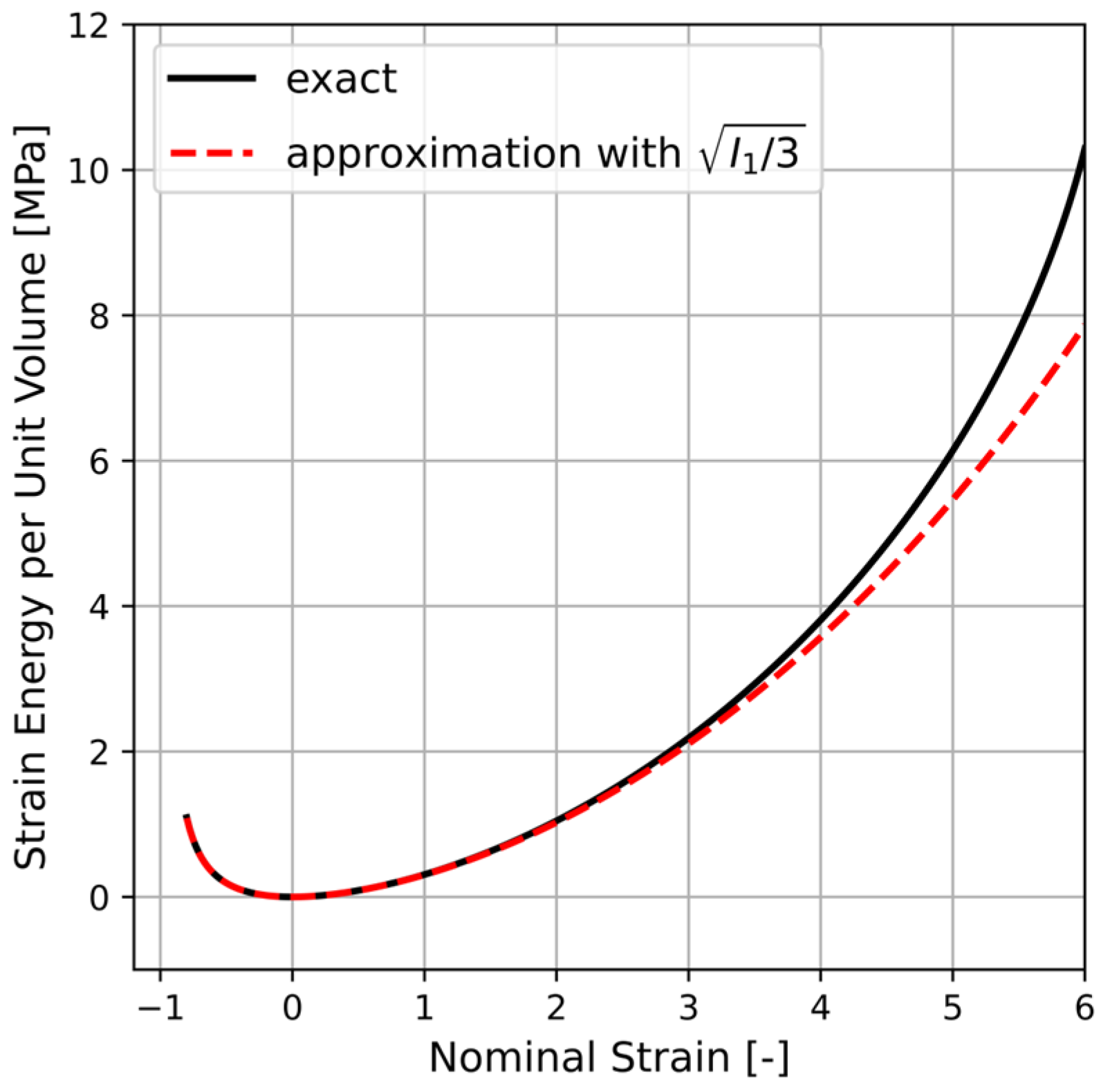
in Equation (A8) is solved numerically in a Python script by incorporating Equation (A1) and the direction cosines given using Equation (A5). The result is indicated by a solid line in Figure A1 where also n ψ c λ ¯ c with λ ¯ c = I 1 / 3   (dashed line) is plotted. It is apparent that the approximation given by Equation (A8) is fairly accurate. Hence, by using the concept of averaging of a single chain micro-variable over all possible chain orientations, the corresponding macroscopic strain energy can be obtained.
Figure A1. Comparison between n ψ c ( λ c ) (solid line) and n ψ c λ ¯ c with λ ¯ c = I 1 / 3   (dashed line) where the integral in the former is solved numerically using Python. The chosen constants are n N k B T = 0.3 and N = 7 (cf. Equation (A4)).
Modelling 05 00027 g0a1
In analogous matter, one can find the contribution of topological constraints (Equation (A2)) to the strain energy of the network. Hence, a relation between the corresponding micro-variable, i.e., the change in the tube cross-section Γ = d 0 / d 2 , and the macroscopic principal stretches λ 1 ,   λ 2 and λ 3 . In continuums mechanic, an area element d A characterized by a unit normal vector N in an initial configuration is related to the deformed (current) configuration according to the Nanson’s Formula d a   n = J   d A   F T N where d a is the area element in the current configuration with the unit normal n . Multiplying each side (dot product) of Equation (A9) by itself yields the squared areal change
d a d A 2 = J 2   F T N . F T N = J 2   N . C 1 N = J 2 j = 1 3 N j 2 λ j 2 ,
with λ 1 2 , λ 2 2 and λ 3 2 as the principal values of the inverse of the right Cauchy–Green tensor C 1 . One can assume that the micro-tube deformation, i.e., the reduction in the tube cross-section Γ = d 0 / d 2 coincides with the macroscopic areal change of the material surface element such that Γ 2 = d a / d A 2 = λ 1 λ 2 λ 3 2 j = 1 3 N j 2 λ j 2 , where J 2 in Equation (A9) is substituted by λ 1 λ 2 λ 3 2 . In order to account for all possible orientations of the normal vector N , we employ the averaging operator v = ( 1 / S u ) S u v   d A u . Hence, with the help of the relation found above for Γ 2 and the direction cosine given using Equation (A5), we obtain
Γ 2 = 1 4 π 0 2 π 0 π sin 2 θ 0 ( λ 2 2 λ 3 2 cos 2 ϕ 0 + λ 1 2 λ 3 2 sin 2 ϕ 0 ) + λ 1 2 λ 2 2 cos 2 θ 0 sin θ 0   d θ 0   d ϕ 0 = I 2 3
in which I 2 = λ 2 2 λ 3 2 + λ 1 2 λ 3 2 + λ 1 2 λ 2 2 is the second invariant of the right Cauchy–Green tensor C . It should be mentioned that Kearsley [59] was apparently the first to notice the relation between the second strain invariant and the average areal change of a surface element in which the average is taken over all possible orientations. According to Equation (A10), the average reduction in the tube cross-section for a chain with an arbitrary initial orientation can be expressed as Γ ¯ = Γ 2 = I 2 / 3 . Subsequently, one can extend Equation (A8) by an extra term that accounts for the effect of topological constraints in the network, i.e., Ψ = n ψ c λ ¯ c + n ψ t Γ ¯ . Hence, substitution of the average micro-variables λ ¯ c = I 1 / 3 and Γ ¯ = I 2 / 3 in the single chain strain energies Equations (A1) and (A2) yields the total strain energy per unit volume of the network
Ψ I 1 , I 2 = n k B T N I 1 3 N β + ln β sinh β   + n k B T α N l / d 0 2 I 2 3 1
The nominal or engineering stress for an incompressible material is given by P i = Ψ / λ i p / λ i with i = 1 ,   2 and 3 [48,60]. In the case where no volume change occurs, p turns out to be a Lagrange multiplier that can be evaluated from the reference state of stress. Note that the strain energy function given using Equation (A11) depends on the first and second invariant of the deformation and hence the chain rule must be applied for the derivation of the nominal stress. In case of a uniaxial deformation, λ 1 = λ and the incompressibility condition λ 1 λ 2 λ 3 = 1 imply that λ 2 = λ 3 = λ 1 / 2 . The hydrostatic pressure p can then be found from the boundary condition P 2 = P 3 = 0 . Consequently, the nominal stress in uniaxial deformation corresponding to the strain energy function Equation (A11) may be written as
P 1 = μ c N 3 I 1 L 1 I 1 / 3 N λ λ 2 + μ t   3 / I 2     1 λ 3
in which the model parameters μ c = n k B T and N are associated with the unconstrained motion of the chains between two cross-links, whereas the constant μ t = n k B T α N l / d 0 2 is related to the tube constraint that models the entanglements.

References

  1. Da Silva, L.F.M.; Öchsner, A.; Adams, R.D. Handbook of Adhesion Technology: Volume 1; Springer: Berlin/Heidelberg, Germany, 2011; ISBN 978-3-642-01168-9. [Google Scholar]
  2. Evangelista Fernandes, P.H.; Nagel, C.; Wulf, A.; Beber, V.C. Mean stress correction and fatigue failure criteria for hyperelastic adhesive joints. J. Adhes. 2024, 100, 219–242. [Google Scholar] [CrossRef]
  3. Fernandes, P.H.E.; Nagel, C.; Wulf, A.; Beber, V.C.; Mayer, B. Compliance-Based Determination of Fatigue Design Curves for Elastomeric Adhesive Joints. Eng 2023, 4, 2615–2639. [Google Scholar] [CrossRef]
  4. Fernandes, P.H.E.; Wulf, A.; Nagel, C.; Beber, V.C. FE-Simulation and Experimental Characterisation of Environmental Effects on the Diffusion and Mechanical Performance of Hyperelastic Adhesive Joints. Eng 2023, 4, 2122–2140. [Google Scholar] [CrossRef]
  5. Da Silva, L.F.M.; Campilho, R.D.S.G. Advances in Numerical Modelling of Adhesive Joints. In Advances in Numerical Modeling of Adhesive Joints; Da Silva, L.F.M., Campilho, R.D.S.G., Eds.; Springer: Berlin/Heidelberg, Germany, 2012; pp. 1–93. ISBN 978-3-642-23607-5. [Google Scholar]
  6. He, X. A review of finite element analysis of adhesively bonded joints. Int. J. Adhes. Adhes. 2011, 31, 248–264. [Google Scholar] [CrossRef]
  7. Hesebeck, O.; Wulf, A. Hyperelastic constitutive modeling with exponential decay and application to a viscoelastic adhesive. Int. J. Solids Struct. 2018, 141–142, 60–72. [Google Scholar] [CrossRef]
  8. Bergström, J. Elasticity/Hyperelasticity. In Mechanics of Solid Polymers; Elsevier: Amsterdam, The Netherlands, 2015; pp. 209–307. ISBN 9780323311502. [Google Scholar]
  9. Mooney, M. A Theory of Large Elastic Deformation. J. Appl. Phys. 1940, 11, 582–592. [Google Scholar] [CrossRef]
  10. Rivlin, R.S.; Saunder, D.W. Large elastic deformations of isotropic materials VII. Experiments on the deformation of rubber. Phil. Trans. R. Soc. Lond. A 1951, 243, 251–288. [Google Scholar] [CrossRef]
  11. Arruda, E.; Boyce, M. A three-dimensional constitutive model for the large stretch behavior of rubber elastic materials. J. Mech. Phys. Solids 1993, 41, 89–412. [Google Scholar] [CrossRef]
  12. Kuhn, W. Beziehungen zwischen Molekülgröße, statistischer Molekülgestalt und elastischen Eigensehaften Hochpolymerer Stoffe. Kolloid-Zeitschrift 1936, 76, 258–271. [Google Scholar] [CrossRef]
  13. Kuhn, W.; Grün, F. Beziehungen zwischen elastischen Konstanten und Dehnungsdoppelbrechung hochelastischer Stoffe. Kolloid-Zeitschrift 1942, 101, 248–271. [Google Scholar] [CrossRef]
  14. James, H.M.; Guth, E. Theory of the Elastic Properties of Rubber. J. Chem. Phys. 1943, 11, 455–481. [Google Scholar] [CrossRef]
  15. Treloar, L.R.G. The Photoelastic Properties of Short-Chain Molecular Networks. Trans. Faraday Soc. 1954, 50, 881. [Google Scholar] [CrossRef]
  16. Witten, T.A.; Rubinstein, M.; Colby, R.H. Reinforcement of rubber by fractal aggregates. J. Phys. II Fr. 1993, 3, 367–383. [Google Scholar] [CrossRef]
  17. Medalia, A.I. Effective Degree of Immobilization of Rubber Occluded within Carbon Black Aggregates. Rubber Chem. Technol. 1972, 45, 1171–1194. [Google Scholar] [CrossRef]
  18. Nunes, R.; Fonseca, J.; Pereira, M.R. Polymer–filler interactions and mechanical properties of a polyurethane elastomer. Polym. Test. 2000, 19, 93–103. [Google Scholar] [CrossRef]
  19. Dong, M.; Li, Q.; Liu, H.; Liu, C.; Wujcik, E.K.; Shao, Q.; Ding, T.; Mai, X.; Shen, C.; Guo, Z. Thermoplastic polyurethane-carbon black nanocomposite coating: Fabrication and solid particle erosion resistance. Polymer 2018, 158, 381–390. [Google Scholar] [CrossRef]
  20. Petrović, Z.S.; Ferguson, J. Polyurethane elastomers. Progress. Polym. Sci. 1991, 16, 695–836. [Google Scholar] [CrossRef]
  21. Mullins, L.; Tobin, N.R. Behavior of Filler-Reinforced Vulcanized Rubbers. Rubber Chem. Technol. 1957, 30, 555. [Google Scholar] [CrossRef]
  22. Mullins, L.; Tobin, N.R. Stress softening in rubber vulcanizates. Part I. Use of a strain amplification factor to describe the elastic behavior of filler-reinforced vulcanized rubber. J. Appl. Polym. Sci. 1965, 9, 2993–3009. [Google Scholar] [CrossRef]
  23. Darabi, E.; Itskov, M. A simple and accurate approximation of the inverse Langevin function. Rheol. Acta 2015, 54, 455–459. [Google Scholar] [CrossRef]
  24. Einstein, A. Eine Neue Bestimmung der Moleküldimensionen. Ph.D. Thesis, ETH Zurich, Zürich, Switzerland, 1906. [Google Scholar]
  25. Batchelor, G.K.; Green, J.T. The determination of the bulk stress in a suspension of spherical particles to order c 2. J. Fluid. Mech. 1972, 56, 401. [Google Scholar] [CrossRef]
  26. Smallwood, H.M. Limiting Law of the Reinforcement of Rubber. J. Appl. Phys. 1944, 15, 758–766. [Google Scholar] [CrossRef]
  27. Huber, G. Universelle Eigenschaften Gefüllter Elastomere; University of Mainz: Mainz, Germany, 1997. [Google Scholar]
  28. Brostow, W. Mechanical Properties. In Physical Properties of Polymers Handbook; Mark, J.E., Ed.; Springer: New York, NY, USA, 2007; pp. 423–445. [Google Scholar]
  29. Kraus, G. Reinforcement of elastomers by carbon black. In Fortschritte der Hochpolymeren-Forschung; Advances in Polymer Science; Springer: Berlin/Heidelberg, Germany, 1971; Volume 8, pp. 155–237. [Google Scholar]
  30. Smith, T.L. Strength of Elastomers. A Perspective. Rubber Chem. Technol. 1978, 51, 225–252. [Google Scholar] [CrossRef]
  31. Oberth, A.E.; Bruenner, R.S. Tear Phenomena around Solid Inclusions in Castable Elastomers. Trans. Soc. Rheol. 1965, 9, 165–185. [Google Scholar] [CrossRef]
  32. Gent, A.N. Detachment of an elastic matrix from a rigid spherical inclusion. J. Mater. Sci. 1980, 15, 2884. [Google Scholar] [CrossRef]
  33. Harwood, J.A.C.; Payne, A.R. Hysteresis and strength of rubbers. J. Appl. Sci. 1968, 12, 889–901. [Google Scholar] [CrossRef]
  34. Kraus, G. Reinforcement of Elastomers by Particulate Fillers. In Science and Technology of Rubber; Kraus, G., Ed.; Academic Press: Cambridge, MA, USA, 1978; pp. 339–365. ISBN 9780122343605. [Google Scholar]
  35. Kraus, G. Reinforcement of elastomers by carbon black. Angew. Makromol. Chem. 1977, 60, 215–248. [Google Scholar] [CrossRef]
  36. Dannenberg, E.M. The Effects of Surface Chemical Interactions on the Properties of Filler-Reinforced Rubbers. Rubber Chem. Technol. 1975, 48, 410–444. [Google Scholar] [CrossRef]
  37. Boonstra, B.B. Role of particulate fillers in elastomer reinforcement: A review. Polymer 1979, 20, 691–704. [Google Scholar] [CrossRef]
  38. Medalia, A.I.; Kraus, G. Reinforcement of Elastomers by Particulate Fillers. In Science and Technology of Rubber, 2nd ed.; Elsevier: Amsterdam, The Netherlands, 1994; pp. 387–418. ISBN 9780080516677. [Google Scholar]
  39. Medalia, A.I. Filler Aggregates and Their Effect on Reinforcement. Rubber Chem. Technol. 1974, 47, 411–433. [Google Scholar] [CrossRef]
  40. Kraus, G. A Structure—Concentration Equivalence Principle in Carbon Black Reinforcement of Elastomers. Polym. Lett. 1970, 8, 601–606. [Google Scholar] [CrossRef]
  41. Kraus, G. A Carbon Black Structure-Concentration Equivalence Principle. Application to Stress-Strain Relationships of Filled Rubbers. Rubber Chem. Technol. 1971, 44, 199–213. [Google Scholar] [CrossRef]
  42. Wolff, S.; Donnet, J.-B. Characterization of Fillers in Vulcanizates According to the Einstein-Guth-Gold Equation. Rubber Chem. Technol. 1990, 63, 32–45. [Google Scholar] [CrossRef]
  43. Hess, W.M.; Ban, L.L.; McDonald, G.C. Carbon Black Morphology: I. Particle Microstructure. II. Automated EM Analysis of Aggregate Size and Shape. Rubber Chem. Technol. 1969, 42, 1209–1234. [Google Scholar] [CrossRef]
  44. Mackenzie, J.K. The Elastic Constants of a Solid containing Spherical Holes. Proc. Phys. Soc. B 1950, 63, 2–11. [Google Scholar] [CrossRef]
  45. Eshelby, J.D. The Determination of the Elastic Field of an Ellipsoidal Inclusion, and Related Problems. Proc. R. Soc. Lond. Ser. A Math. Phys. 1957, 241, 376–396. [Google Scholar]
  46. Krichen, S.; Liu, L.; Sharma, P. Liquid inclusions in soft materials: Capillary effect, mechanical stiffening and enhanced electromechanical response. J. Mech. Phys. Solids 2019, 127, 332–357. [Google Scholar] [CrossRef]
  47. Steinmann, P.; Hossain, M.; Possart, G. Hyperelastic models for rubber-like materials: Consistent tangent operators and suitability for Treloar’s data. Arch. Appl. Mech. 2012, 82, 1183–1217. [Google Scholar] [CrossRef]
  48. Edwards, S.F.; Vilgis, T.A. The tube model theory of rubber elasticity. Rep. Prog. Phys. 1988, 51, 243–297. [Google Scholar] [CrossRef]
  49. Medalia, A.I. Morphology of aggregates: VI. Effective volume of aggregates of carbon black from electron microscopy; Application to vehicle absorption and to die swell of filled rubber. J. Colloid. Interface Sci. 1970, 32, 115–131. [Google Scholar] [CrossRef]
  50. Edwards, S.F. The statistical mechanics of polymerized material. Proc. Phys. Soc. 1967, 92, 9–16. [Google Scholar] [CrossRef]
  51. Doi, M.; Edwards, S. The Theory of Polymer Dynamics; Clarendon Press: Oxford, UK, 1986. [Google Scholar]
  52. Miehe, C. A micro-macro approach to rubber-like materials? Part I: The non-affine micro-sphere model of rubber elasticity. J. Mech. Phys. Solids 2004, 52, 2617–2660. [Google Scholar] [CrossRef]
  53. Flory, P.J. Thermodynamic Relations for High Elastic Materials. Trans. Faraday Soc. 1961, 57, 829–838. [Google Scholar] [CrossRef]
  54. Flory, P.J.; Rehner, J. Statistical Mechanics of Cross-Linked Polymer Networks I. Rubberlike Elasticity. J. Chem. Phys. 1943, 11, 512–520. [Google Scholar] [CrossRef]
  55. Wu, P.D.; van der Giessen, E. On improved 3-D non-Gaussian network models for rubber elasticity. Mech. Res. 1992, 19, 427–433. [Google Scholar] [CrossRef]
  56. Wu, P.D.; van der Giessen, E. On improved network models for rubber elasticity and their applications to orientation hardening in glassy polymers. J. Mech. Phys. Solids 1993, 41, 427–456. [Google Scholar] [CrossRef]
  57. Beatty, M.F. An Average-Stretch Full-Network Model for Rubber Elasticity. J. Elast. 2003, 70, 65–86. [Google Scholar] [CrossRef]
  58. Dickie, R.A.; Smith, T.L. Viscoelastic Properties of a Rubber Vulcanizate Under Large Deformations in Equal Biaxial Tension, Pure Shear, and Simple Tension. Trans. Soc. Rheol. 1971, 15, 91–110. [Google Scholar] [CrossRef]
  59. Kearsley, E.A. Note: Strain Invariants Expressed as Average Stretches. J. Rheol. 1989, 33, 757–760. [Google Scholar] [CrossRef]
  60. Treloar, L.R.G. The Physics of Rubber Elasticity, 3rd ed.; Clarendon Press: Oxford, UK, 1975; ISBN 0198513550. [Google Scholar]
Figure 1. Scanning electron microscopy (SEM) images of the fillers used in the PU composites, namely Aerosil 200 (upper left), Special Black 250 (upper right) and Printex 30 (bottom). The images are taken at 30,000× magnification. The scale bars in all three images correspond to 1 µm.
Modelling 05 00027 g001
Figure 2. Three-roller mill used for the dispersion of Printex® 30. The black high-viscose substance shown in both images is the resulting paste after the dispersion of carbon black in the B component of the PU system.
Modelling 05 00027 g002
Figure 3. Image of the test specimens used for uniaxial tensile tests. The dimensions of the specimens correspond to those of standard specimens of type 5A in ISO 527 and type S2 in ISO 53504. The image corresponds to a PU-nanocomposite filled with 10 wt% Printex® 30.
Modelling 05 00027 g003
Figure 4. Scanning electron microscopy (SEM) images taken from the cross-section of the prepared test specimens at 2000× magnification. The upper left and upper right images correspond to the unfilled sample and the PU-nanocomposite including 5 wt% Printex® 30, respectively. The samples filled with 10 wt% and 20 wt% Printex® 30 are represented by the lower left and right images. The scale bars in the images correspond to 20 µm.
Modelling 05 00027 g004
Figure 5. Test setup for quasi-static tensile tests (left). Extension of an unfilled specimen (pure PU) according to DIN EN ISO 527-2 (right).
Modelling 05 00027 g005
Figure 6. Measured uniaxial stress–strain curves of PU-nanocomposites filled with 5, 10, 15, and 20% (wt%) Printex® 30 (solid curves). The dashed curve corresponds to the pure (unfilled) polyurethane sample.
Modelling 05 00027 g006
Figure 7. Measured tensile strength, corresponding to the maximal nominal stress experienced by a sample, of PU-nanocomposites filled with 0, 5, 10, 15, and 20% (wt%) Printex® 30.
Modelling 05 00027 g007
Figure 8. Stress at 200, 300, and 400% extension as a function of the effective filler volume loading a ϕ for PU-nanocomposites filled with 0, 5, 10, 15, and 20% (wt%) Printex® 30. The symbols correspond to the measured data and the solid lines are polynomial functions of the effective volume loading. Note that the symbols at a ϕ = 0, 0.031, 0.062, 0.093, and 0.124 correspond to the samples filled with 0, 5, 10, 15 and 20% (wt%) Printex® 30, respectively.
Modelling 05 00027 g008
Figure 9. Representative measured uniaxial stress–strain curves of unfilled PU and PU-nanocomposites filled with 1% (wt%) Printex® 30, Special Black 250 (SS250), and Aerosil® 200 (fumed silica).
Modelling 05 00027 g009
Figure 10. The effect of 1 wt% filler on the small strain (Young’s) modulus and the tensile strength of the PU-nanocomposites represented by circles and squares, respectively. The corresponding volume fraction for both carbon blacks, i.e., Printex® 30 and Special Black 250, is ϕ = 0.005 . For Aerosil® 200, ϕ = 0.004 .
Modelling 05 00027 g010
Figure 11. Uniaxial stress–strain curves of the unfilled PU and PU-nanocomposites filled with 1 wt% Printex® 30 (P30) and Aerosil® 200 (A200). Symbols and lines correspond to the measured data and fit of the model without strain amplification (Equation (3)), respectively.
Modelling 05 00027 g011
Figure 12. Comparison between the uniaxial tension data and the constitutive relation Equation (3) for the PU composites filled with 5, 15, and 20 wt% Printex® 30. The dashed and solid lines correspond to the test results and the model fits, respectively. The inset shows the comparison at small strain values for the samples filled with 5 and 20 wt% carbon black.
Modelling 05 00027 g012
Figure 13. Comparison between the uniaxial tension data (circles), the constitutive relation Equation (3) (dashed line) and the modified constitutive relation (Equation (3)) (solid line) for a PU composite filled with 5 wt% Printex® 30. The inset shows the comparison in the small strain region. Note that Equation (3) corresponds to Equation (4) with X = 1 . The term X > 1 refers to the constant strain amplification factor X = 1 / ( 1 ϕ e f f ) .
Modelling 05 00027 g013
Figure 14. Comparison between the uniaxial tension data (circles) and different constitutive relations for a PU sample filled with 20 wt% Printex® 30. The constitutive relation Equation (3), corresponding to a strain amplification factor of unity, is represented by the dashed line. The solid and the dotted line correspond to the modified constitutive relation (Equation (4)) with the constant strain amplification X = 1 / ( 1 ϕ e f f ) and Equation (7) where the deformation-dependent amplification factor X ( ϵ ) is given by Equation (8), respectively. The inset shows the comparison in the small strain region.
Modelling 05 00027 g014
Figure 15. Stress–strain curves of uniaxial tensile test on Sikaflex-250 UHM at a strain rate of approximately 0.1 s 1 at room temperature and respective fits of the model without strain amplification ( X = 1 ) , with constant strain amplification ( X = c o n s t . ) and with deformation-dependent strain amplification ( X = X ( ϵ ) ) .
Modelling 05 00027 g015
Table 1. Key filler-related parameters of PU-nanocomposites.
FillerWeight Fraction (wt%)Volume Fraction ϕ [−]Density [g/cm3]Specific Surface [m2/g]Oil Absorption (DBP) Number [mL/100 g]Average Primary Particle Size [nm]
10.0051.98010827
50.03
Printex®30100.06
150.09
200.12
SS 25010.0051.9484547
Aerosil®20010.0042.2200-12
Table 2. Parameters for the model without strain amplification (Equation (3)) for Figure 11.
μ c   [ M P a ] μ t   [ M P a ] N   [ ] R 2   [ ]
Unfilled PU 0.30 1.5 6.65 0.9993
PU + 1 wt% A200 0.31 0.93 6 0.9993
PU + 1 wt% P30 0.3 0.98 5.8 0.9990
Table 3. Parameters for the model without strain amplification (Equation (3)).
μ c   [ m P a ] μ t   [ m P a ] N   [ ] R 2   [ ]
PU + 5 wt% 0.49   0.65 6 0.9990
PU + 15 wt% 0.80   0.27 7 0.9978
PU + 20 wt% 1.01 0.65 7 0.9946
Table 4. Parameters for the model with constant strain amplification (Equation (4)) for Figure 13.
μ c   [ M P a ] μ t   [ M P a ] N   [ ] ϕ e f f   [ ]
PU + 5 wt% 0.2 1.35 16.29 0.64
Table 5. Parameters for the model with constant strain amplification (Equation (4)) for Figure 14.
μ c   [ M P a ] μ t   [ M P a ] N   [ ] ϕ e f f   [ ]
PU + 20 wt% 0.2 1.72 71.96 0.84
Table 6. Parameters for the model with deformation-dependent strain amplification (Equation (7)) for Figure 14.
μ c   [ M P a ] μ t   [ M P a ] X 0   [ ] X   [ ] z   [ ] N   [ ]
PU + 20 wt% 0.41 1.62 2.85 0.45 0.33.9
Table 7. Model parameters for fitting of the commercial adhesive SikaFlex 250 UHM at RT.
Parameter μ c   [ M P a ] μ t   [ M P a ] X 0   [ ] X   [ ] z   [ ] N   [ ]
AdhesiveModel
SikaFlex 250 UHM RT Model + X ( ϵ ) 0.572.121.083.330.7915.53
Model + const .   X 2.0728.50.46--3.27
Model   without   X 2.2417.2---3.6 × 10⁴
Disclaimer/Publisher’s Note: The statements, opinions and data contained in all publications are solely those of the individual author(s) and contributor(s) and not of MDPI and/or the editor(s). MDPI and/or the editor(s) disclaim responsibility for any injury to people or property resulting from any ideas, methods, instructions or products referred to in the content.

