Article

Stress–Strength Reliability of the Type P(X < Y) for Birnbaum–Saunders Components: A General Result, Simulations and Real Data Set Applications

by
Felipe S. Quintino
1,
Luan Carlos de Sena Monteiro Ozelim
2,*,
Tiago A. da Fonseca
3 and
Pushpa Narayan Rathie
1
1
Department of Statistics, University of Brasilia, Brasília 70910-900, Brazil
2
Department of Civil and Environmental Engineering, University of Brasilia, Brasília 70910-900, Brazil
3
Gama Engineering College, University of Brasilia, Brasília 72444-240, Brazil
*
Author to whom correspondence should be addressed.
Modelling 2024, 5(1), 223-237; https://doi.org/10.3390/modelling5010012
Submission received: 30 December 2023 / Revised: 8 February 2024 / Accepted: 13 February 2024 / Published: 15 February 2024

Abstract

:
An exact expression for R = P ( X < Y ) has been obtained when X and Y are independent and follow Birnbaum–Saunders (BS) distributions. Using some special functions, it was possible to express R analytically with minimal parameter restrictions. Monte Carlo simulations and two applications considering real datasets were carried out to show the performance of the BS models in reliability scenarios. The new expressions are accurate and easy to use, making the results of interest to practitioners using BS models.

1. Introduction

The Birnbaum–Saunders (BS) fatigue-life model with two parameters was originally introduced in [1] and stems from the principles of renewal theory, focusing on the count of cycles required to surpass a critical threshold and induce fatigue crack propagation. In the same year, those same authors [2] provided maximum likelihood estimates (MLE) for BS model parameters. Later, Desmond [3] presented an alternative derivation of the distribution using a biological model and relaxing several of the assumptions made in [1], and Desmond [4] further studied how the Birnbaum–Saunders distribution could be related to inverse Gaussian distributions. The cumulative distribution function (CDF) of the Birnbaum–Saunders ( B S ( α , β ) ) model is given by:
F ( t ; α , β ) = Φ 1 α ξ t β , t > 0 ,
where Φ ( · ) is the CDF of a standard normal distribution, α > 0 and β > 0 are the shape and scale parameters, respectively, and
ξ ( x ) = x 1 x , x > 0 .
In this work, the focus is on the stress–strength reliability metric P ( X < Y ) (cf. [5]) when both X and Y are distributed as B S ( α , β ) random variables. In broad terms, one may be interested in the likelihood of a system or component failing based on a comparison between the applied stress and the system’s strength. Let us consider stress, denoted as variable Y, and strength, denoted as variable X. Assuming these are independent continuous random variables (RVs) with probability density function (PDF) f Y and CDF F X , respectively, the stress–strength probability (also referred to as reliability) is defined as follows:
R : = P ( X < Y ) = F X ( x ) f Y ( x ) d x .
This theory finds numerous applications, including statistics, economics, engineering and decision theory, and the reader may refer to the seminal work by Kotz et al. [5] for additional details.
For instance, when considering the reliability of a particular system, such a metric can indicate the likelihood of one system performing better than another concerning reliability or failure rates. Thus, specialists might utilise this metric to determine which system is more reliable for a specific application. Also, financial analysts might employ this metric to evaluate the relative risk linked with various investment strategies or assets. In contrast, manufacturing sectors could utilise this measure to appraise the effectiveness of quality control methods or production processes, thereby pinpointing areas for enhancement and optimising operations to enhance product quality and customer satisfaction.
In essence, the significance of reliability metrics such as R lies in their capacity to enable quantitative assessments for comparison, evaluation and informed decision making in intricate and uncertain circumstances. This, in turn, facilitates improved risk management, allocation of resources and optimisation across a broad spectrum of domains.
The stress–strength reliability metric when X and Y are independent RVs with distributions, respectively, B S ( α x , β x ) and B S ( α y , β y ) , was studied by Xiuyun et al. [6], who derived an expression for the stress–strength probability R based on progressively Type II-censored samples. They presented an approximated expression for R when α x = α y = α . MLE and Bayesian estimators were also studied in [6]. In the present paper, it is of interest to explore cases without such parameter restrictions and in an exact and compact framework through the use of generalised hypergeometric special functions like the ones proposed by Rathie et al. [7].
Special functions are widely studied in the literature, such as the cases of the generalised hypergeometric function, Meijer’s G-function, Fox’s H-function, modified Bessel K ν -function of the third kind (see Definitions 1.1, 1.5, 1.6 and 1.11 in [8]), I ^ -function ([7]). Thus, the results are hereby obtained using such functions and their properties. In the context of stress–strength reliability, the use of special functions is a way to provide expressions for R with fewer parameter restrictions (see [9] for example).
The paper is organised as follows: in Section 2, some preliminary concepts are presented, especially the definition of some useful special functions and of the Birnbaum–Saunders distribution (its density and properties of interest). Section 3 deals with the derivation of R when X and Y are independent Birnbaum–Saunders RVs as well as the estimation of R. In Section 4, Monte-Carlo simulations are presented to show the correctness of the analytical expressions derived. Besides, in Section 4, the modelling of two real datasets which account for the strength of different-length carbon fibres and daily wind speeds in two Atlantic coastal cities are presented. Then, conclusions are presented in Section 5.

2. Preliminaries

In this section, some definitions and results, which will be used subsequently, are presented.

2.1. Special Functions and Mellin Transforms

The Fox’s H-function (cf. Definition 1.1 in [8]) is defined by:
H p , q m , n z | ( a 1 , A 1 ) , , ( a p , A p ) ( b 1 , B 1 ) , , ( b q , B q ) = 1 2 π i L k = 1 m Γ ( b j + B j s ) j = 1 n Γ ( 1 a j A j s ) k = m + 1 q Γ ( 1 b j B j s ) j = n + 1 p Γ ( a j + A j s ) z s d s ,
where 0 m q , 0 n p (not both m and n simultaneously zero), Γ ( · ) is the gamma function and i stands for square root of ( 1 ) , A j > 0 ( j = 1 , , p ), B k > 0 ( k = 1 , , q ), a j and b k are complex numbers such that no poles of Γ ( b k + B k s ) ( k = 1 , , m ) coincide with poles of Γ ( 1 a j A j s ) ( j = 1 , , n ) . L is a suitable contour w i to w + i , w R , separating the poles of the two types mentioned above. For more details, see [8].
The Meijer’s G-function is a particular case of the H-function and can be defined (Definition 1.5 in 1.5 [8]) by:
G p , q m , n z | a 1 , , a p b 1 , , b q = 1 2 π i L k = 1 m Γ ( b k s ) j = 1 n Γ ( 1 a j + s ) k = m + 1 q Γ ( 1 b k + s ) j = n + 1 p Γ ( a j s ) z s d s ,
where x 0 , an empty product is interpreted as unity, 0 m q , 0 n p (not both m and n simultaneously zero). The parameters a j ( j = 1 , , n ) and b k ( k = 1 , , m ) are such that no poles of j = 1 n Γ ( b k s ) coincide with poles of j = 1 n Γ ( 1 a j + s ) . Refer to the study by [10] for details about the contour L and about the convergence conditions of the integral.
Let M [ f ] ( s ) denote the Mellin transform of a function f, which can be mathematically defined as (cf. [8]):
M [ f ] ( s ) = 0 t s 1 f ( t ) d t ,
provided that the integral converges. The inverse Mellin transform is obtained by the contour integral:
f ( x ) = M 1 [ M [ f ] ] ( x ) = 1 2 π i c i c + i x s M [ f ] ( s ) d s .
Rathie et al. [7] proposed a generalisation of the H-function, thereby named the I ^ function, defined as a contour complex integral which contains H-functions in their integrands. The function is given by:
I ^ m z ( a ¯ m , 1 , a ^ m , 1 , A ¯ m , 1 ) , ( a ¯ m , 2 , a ^ m , 2 , A ¯ m , 2 ) , ( a ¯ m , 3 , a ^ m , 3 , A ¯ m , 3 ) ( b ¯ m , 1 , b ^ m , 1 , B ¯ m , 1 ) , ( b ¯ m , 2 , b ^ m , 2 , B ¯ m , 2 ) ( γ ¯ m , Γ ¯ m , π ¯ m , Π ¯ m , ρ ¯ m , σ ¯ m ) ( α ¯ m , β ¯ m , Λ ¯ m , Θ ¯ m , ζ ¯ m , η ¯ m ) = 1 2 π i L Ψ ( s ) z s d s ,
in which Ψ ( s ) is the Mellin transform of the new function and can be explicitly given as:
Ψ ( s ) = j = 1 m ( α ¯ j s + β ¯ j ) Λ ¯ j s + Θ ¯ j e ζ ¯ j s + η ¯ j × × H 3 , 2 2 , 1 ( γ ¯ j + Γ ¯ j s ) π ¯ j + Π ¯ j s ( a ¯ j , 1 + a ^ j , 1 s , A ¯ j , 1 ) , ( a ¯ j , 2 + a ^ j , 2 s , A ¯ j , 2 ) , ( a ¯ j , 3 + a ^ j , 3 s , A ¯ j , 3 ) ( b ¯ j , 1 + b ^ j , 1 s , B ¯ j , 1 ) , ( b ¯ j , 2 + b ^ j , 2 s , B ¯ j , 2 ) ρ ¯ j s + σ ¯ j ,
where A ¯ j , k and B ¯ j , k are assumed to be positive real quantities, the a ¯ j , k , a ^ j , k , b ¯ j , k , b ^ j , k , Π ¯ j , π ¯ j , Γ ¯ j , γ ¯ j , ρ ¯ j , σ ¯ j , α ¯ j , β ¯ j , Λ ¯ j , Θ ¯ j , ζ ¯ j , η ¯ j , j = 1 , , m are real numbers. The contour L runs from c i to c + i , where c is a real number, and exists in accordance with Mellin inversion theorem, taking into account all the singularities.

2.2. The BS Model

The PDF of the BS model is given by:
f ( t ) = ϕ 1 α ξ t β 1 α ξ t β 1 β , t > 0 ,
which can also be explicitly expressed as:
f ( t ; α , β ) = 1 2 2 π α β β t 1 / 2 + β t 3 / 2 exp 1 2 α 2 t β + β t 2 , t > 0 ,
since ϕ ( · ) denotes the PDF of a standard normal distribution. Figure 1 shows the PDF given in (7) and the CDF given in (1) for some choices of parameters.
From [11,12], it follows that:
E [ T p ] = β p I ( p , α ) ,
where T B S ( α , β ) and
I ( p , α ) = K p + 1 / 2 ( α 2 ) + K p 1 / 2 ( α 2 ) 2 K 1 / 2 ( α 2 ) ,
and K ν ( z ) is the modified Bessel function of the third kind (see Definition 1.11 in [8]). Also, literature [8] (p. 24) indicates that:
K ν ( z ) = 1 2 H 0 , 2 2 , 0 z 2 4 ( ν / 2 , 1 ) , ( ν / 2 , 1 ) = 1 2 G 0 , 2 2 , 0 z 2 4 ν 2 , ν 2 .
Equation (11) will be used to obtain an expression for the stress–strength probability R in terms of I ^ functions.

3. Stress–Strength Probability for BS Models

Let X and Y be independent random variables with X B S ( α x , β x ) , and Y B S ( α y , β y ) , α j , β j R + ( j { x , y } ). The stress–strength probability is given by:
R = P ( X < Y ) = 0 F X ( t ; α x , β x ) f Y ( t ; α y , β y ) d t .
As described, Xiuyun et al. [6] presented an approximate expression for (12) when α 1 = α 2 = α . The results hereby obtained, on the other hand, will not consider such restrictions.
Thus, it follows from (7) and (12) that:
R = 0 Φ 1 α x ξ t β x ϕ 1 α y ξ t β y 1 α y ξ t β y 1 β y d t
At first, let us consider a special case where ξ t β x = ξ t β y = u . Then, β x = β y , which implies:
R = Φ 1 α x u ϕ 1 α y u 1 α y d u .
In this case, it is worth noticing that:
  • Φ 1 α x u is the CDF of V x N ( 0 , α x ) ;
  • ϕ 1 α y u is the PDF of V y N ( 0 , α y ) .
Thus, since V x and V y are independent:
R = P ( V x < V y ) = P ( V x V y < 0 ) = 1 2 ,
which suggests the following remark:
Remark 1.
If β x = β x = β , the stress–strength reliability metric in (12) is given by R = 0.5 .
Coming back to the definition of R given in (12), then:
R = P ( X < Y ) = P X Y < 1 ,
since Y is a positive RV. One may look for the CDF of W = X Y to investigate R. The Mellin transform, as defined in (4), of the PDF f W is given by:
M [ f W ] ( s ) = M [ f X ] ( s ) M [ f Y ] ( 2 s ) .
One may refer to [13] for further details on the properties of Mellin transforms in the context of the algebra of random variables.
From (9):
M [ f X ] ( s ) = E [ X s 1 ] = β x s 1 I ( s 1 , α x )
and, similarly,
M [ f Y ] ( s ) = E [ Y s 1 ] = β y s 1 I ( s 1 , α y ) .
Then, by inverting the Mellin transform:
f W ( z ) = β y β x 1 2 π i L I ( s 1 , α x ) I ( 1 s , α y ) β y z β x s d s .
The direct integration of the PDF f W ( z ) leads to:
F W ( z ) = 0 z f W ( w ) d w = β y β x 1 2 π i L I ( s 1 , α x ) I ( 1 s , α y ) β y β x s 0 z w s d w d s = β y β x 1 2 π i L I ( s 1 , α x ) I ( 1 s , α y ) β y β x s z 1 s 1 s d s ,
provided that R e ( 1 s ) > 0 ( R e ( z ) is the real part of z). Then:
F W ( z ) = z β y β x 1 2 π i L I ( s 1 , α x ) I ( 1 s , α y ) 1 s β y z β x s d s ,
which implies:
R = P X 1 X 2 < 1 = F W ( 1 ) = β y β x 1 2 π i L I ( s 1 , α x ) I ( 1 s , α y ) 1 s β y β x s d s .
Using (10) and (11), the inner part of the integral (13) becomes:
I ( s 1 , α x ) I ( 1 s , α y ) = 1 16 1 K 1 / 2 ( α x 2 ) K 1 / 2 ( α y 2 ) × G 0 , 2 2 , 0 α x 4 4 s 1 / 2 2 , s 1 / 2 2 + G 0 , 2 2 , 0 α x 4 4 s 3 / 2 2 , s 3 / 2 2 × G 0 , 2 2 , 0 α y 4 4 s 1 / 2 2 , s 1 / 2 2 + G 0 , 2 2 , 0 α y 4 4 s 3 / 2 2 , s 3 / 2 2 .
This implies that R is the sum of four I ^ functions (5), proving the following result:
Theorem 1.
Let X B S ( α x , β x ) and Y B S ( α y , β y ) be independent RVs, α x , α x , β x , β y R + . Then:
R = P ( X < Y ) = 1 16 β y β x 1 K 1 / 2 ( α x 2 ) K 1 / 2 ( α y 2 ) I 1 + I 2 + I 3 + I 4 ,
where, for k = 1 , , 4 :
I k = I ^ 2 β y β x { ( 0 , 0 , 0 ) , ( 1 , 0 , 0 ) , ( 1 , 0 , 0 ) } , { ( 0 , 0 , 0 ) , ( 1 , 0 , 0 ) , ( 1 , 0 , 0 ) } { ( ν 1 , k / 2 , 1 / 2 , 1 ) , ( ν 1 , k / 2 , 1 / 2 , 1 ) } , { ( ν 2 , k / 2 , 1 / 2 , 1 ) , ( ν 2 , k / 2 , 1 / 2 , 1 ) } { ( α x 4 / 4 , 0 , 1 , 0 , 0 , 1 ) } , { ( α y 4 / 4 , 0 , 1 , 0 , 0 , 1 ) } { ( 1 , 1 , 0 , 1 , 0 , 0 ) } , { ( 0 , 1 , 0 , 1 , 0 , 0 ) } ,
in which:
ν 1 , k = 1 2 , k { 1 , 2 } , 3 2 , k { 3 , 4 } ,
and
ν 2 , k = 1 2 , k { 1 , 3 } , 3 2 , k { 2 , 4 } .

Estimation

Let X B S ( α x , β x ) and Y B S ( α y , β y ) be independent RVs. It is of interest to estimate R = P ( X < Y ) based on random samples of X and Y. For this, estimates of θ = ( α x , α y , β x , β y ) are required. For simplicity of notation, let x = ( x 1 , , x n ) and y = ( y 1 , , y m ) denote observed random samples of X and Y, respectively.
The log-likelihood function, denoted by l ( θ ) : = l ( θ ; x , y ) , is given by
l ( θ ) = n ( log α x + log β x ) m ( log α y + log β y ) + i = 1 n 1 2 α x 2 ξ 2 t i β x + log ξ t i β x + j = 1 m 1 2 α y 2 ξ 2 u j β y + log ξ u j β y .
The maximum likelihood estimator (MLE) of ( α , β ) was presented in [2]. In the present paper, two independent samples are considered with no parameter equality constraint (as α x = α y considered by [6]), such that θ ^ is obtained directly by the MLEs ( α ^ x , β ^ x ) and ( α ^ y , β ^ y ) .
Remark 2.
The MLE of R is obtained using the invariance property of MLE. This is due to the Theorem 1 that describes R in terms of I ^ functions (which are integrals, hence continuous and measurable functions), that is, using the estimates α ^ x , α ^ y β ^ x and β ^ y . Then, from (14):
R ^ M L E = R ( α ^ x , α ^ y , β ^ x , β ^ y ) .
Algorithm 1 describes the approach used in the next section to obtain bootstrap confidence intervals of R.    
Algorithm 1: Let x and y be samples of sizes n and m, respectively, and a positive integer M.
Step 1 
Generate independent bootstrap samples x i and y i from x and y (or directly sample from distributions if true parameters are known).
Step 2 
Compute the estimate θ ^ i = ( α ^ x , i , α ^ y , i , β ^ x , i , β ^ y , i ) based on x i and y i .
Step 3 
Obtain R ^ i = R ^ ( θ ^ i ) by (14).
Step 4 
Repeat steps 1 to 3 M times.
Step 5 
The approximate 100 ( 1 α ) % confidence interval of R is given by  [ R ^ M ( α / 2 ) , R ^ M ( 1 α / 2 ) ] , where  R ^ M ( α ) G ^ 1 ( α )  and   G ^  is the cumulative distribution function of R ^ considering all  i = 1 , . . . , M samples.
It is also possible to calculate the mean of the estimates obtained in Algorithm 1, denoting this mean as R ^ b o o t = M 1 i = 1 M R ^ i . It is clear that R ^ M L E is the value of R ^ i when x = x i and y = y i , i.e., when the full sample is used to estimate the parameters of the distribution. In the following section, the estimates for both R ^ M L E and R ^ b o o t are obtained. When matched data are present ( m = n ), these results can be compared with a nonparametric estimator denoted as R ^ N P , which is defined as:
R ^ N P = 1 n j = 1 n 1 x j y j ,
where 1 A denotes the indicator function on the set A.

4. Applications

Monte Carlo simulations are presented to assess the estimation of R for the BS model as well as the modelling of two real data sets involving different-length carbon fibres and daily wind speeds in two Atlantic coastal cities. All the applications have been devised to show the full capabilities of the expressions hereby developed, and readers may inquire about the codes used directly to the corresponding author.

4.1. Monte Carlo Simulations

In this subsection, a Monte Carlo simulation study is carried out to evaluate the Bootstrap MLE R ^ b o o t , described in Algorithm 1. Additionally, the assessment of the estimates of α x , β x , α y and β y are also considered. The following fixed parameters are considered for the simulations:
  • True population parameters ( α x , β x , α y ) = ( 0.3 , 35 , 0.5 ) and β y { 27.5 , 30 , 32.5 , 37.5 } ;
  • M = 100 Monte Carlo replications of samples x and y directly sampled from true distributions since the parameters are known;
  • sample sizes m = n { 25 , 100 , 500 , 1000 } .
Aiming to study the Monte Carlo MLEs, the bias and root mean squared error (RMSE) of each estimated value with respect to their true population’s values are computed. The simulation study was programmed in Python. The simulation results of R ^ b o o t are presented in Table 1. Figure 2 and Figure 3 present the bias and RMSE for each estimated parameter. In short, each time Step 2 in Algorithm 1 is run, one ends up having estimates of the parameters α x , β x , α y and β y . After M = 100 runs, there are 100 values which are compared to the true population’s values mentioned before. Observe that by increasing the sample size n, the bias and RMSE of the Monte Carlo simulations decrease.

4.2. Real Data Set

Taking advantage of real data previously analysed in the literature, two applications are presented. The validity of the model for both datasets is studied and it is shown that the BS distribution presents a good fit in both cases.

4.2.1. Carbon Fibres

In the work of Bader and Priest [14], single carbon fibres were tested under tension at gauge lengths of 20 mm and 10 mm, having their strength measured in GPa. The data for both lengths are compared to assess which is statistically higher than the other. These data sets were modelled previously in several works (see, for example, [15]). For the convenience of the reader, data sets of length 20 mm ( x ) and length 10 mm ( y ) are presented below:
x = ( 1.312 , 1.314 , 1.479 , 1.552 , 1.700 , 1.803 , 1.861 , 1.865 , 1.944 , 1.958 , 1.966 , 1.977 , 2.006 , 2.021 , 2.027 , 2.055 , 2.063 , 2.098 , 2.140 , 2.179 , 2.224 , 2.240 , 2.253 , 2.270 , 2.272 , 2.274 , 2.301 , 2.301 , 2.359 , 2.382 , 2.382 , 2.426 , 2.434 , 2.435 , 2.478 , 2.490 , 2.511 , 2.514 , 2.535 , 2.554 , 2.566 , 2.570 , 2.586 , 2.629 , 2.633 , 2.642 , 2.648 , 2.684 , 2.697 , 2.726 , 2.770 , 2.773 , 2.800 , 2.809 , 2.818 , 2.821 , 2.848 , 2.880 , 2.954 , 3.012 , 3.067 , 3.084 , 3.090 , 3.096 , 3.128 , 3.233 , 3.433 , 3.585 , 3.585 )
and
y = ( 1.901 , 2.132 , 2.203 , 2.228 , 2.257 , 2.350 , 2.361 , 2.396 , 2.397 , 2.445 , 2.454 , 2.474 , 2.518 , 2.522 , 2.525 , 2.532 , 2.575 , 2.614 , 2.616 , 2.618 , 2.624 , 2.659 , 2.675 , 2.738 , 2.740 , 2.856 , 2.917 , 2.928 , 2.937 , 2.937 , 2.977 , 2.996 , 3.030 , 3.125 , 3.139 , 3.145 , 3.220 , 3.223 , 3.235 , 3.243 , 3.264 , 3.272 , 3.294 , 3.332 , 3.346 , 3.377 , 3.408 , 3.435 , 3.493 , 3.501 , 3.537 , 3.554 , 3.562 , 3.628 , 3.852 , 3.871 , 3.886 , 3.971 , 4.024 , 4.027 , 4.225 , 4.395 , 5.020 ) .
Descriptive statistics for x and y are presented in Table 2. The boxplot in Figure 4 shows that the data in x are a bit skewed to the right while the data in y are closer to being symmetric. Computing the value of the statistic R is important to quantitatively assess the differences observed in the data sets.
As the data sets have positive support, the BS distribution is a candidate to model such data sets. Let us assume that x and y are observed samples of X B S ( α x , β x ) and Y B S ( α y , β y ) , respectively. Estimates of parameters α x , α y , β x and β y are presented in Table 3 as well as the p-value of the Kolmogorov–Smirnov (KS) test. The results indicate that it is not possible to reject the null hypothesis that BS models the CDF. Figure 5 shows the fit of distributions to data sets.
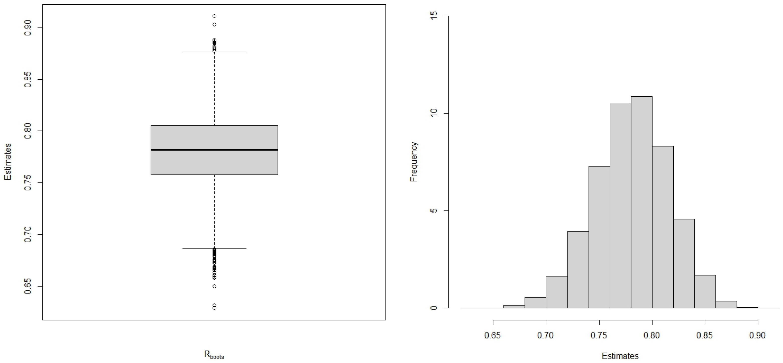
Using Theorem 1 and Algorithm 1, the values of R ^ M L E = 0.7802 , R ^ b o o t s = 0.7808 and the 95 % bootstrap confidence interval ( 0.7092 , 0.8472 ) were obtained. The spread of the bootstrap estimates can be assessed in Figure 6. From the results, it is possible to say that since P ( X < Y ) > 0.5 and 0.5 is not within the CI of the Bootstrap estimates, carbon fibres with a length of 20 mm (sampled from X) show less strength when compared to carbon fibres with a length of 10 mm (sampled from Y).
As mentioned, this dataset has already been analysed in the stress–strength context previously. Valiollahi et al. [15] estimated R after transforming the original data (so that the transformed data had the same scale parameter) and modelling it using the Weibull distribution. They considered MLE, approximate MLE (AML) and Bayes estimator obtaining the values 0.5002 , 0.5172 and 0.5221 , respectively. They also obtained the 95% Boot-p and Boot-t confidence intervals as ( 0.4758 , 0.5789 ) and ( 0.4726 , 0.5823 ) . Their results cannot provide conclusive evidence of the true problem, as the transformation severely impairs the reliability calculations (now P ( X < Y ) = 0.5 is within the CI). In the present analysis, such a transformation is not needed since the BS distribution was a good candidate for modelling the data and Theorem 1 does not require equality of parameters between x and y . To compare the findings of the present study with their transformed datasets, using Tables 4 and 5 of [15], it was estimated that X B S ( 0.2138 , 0.9040 ) , Y B S ( 0.1983 , 0.9051 ) and R ^ M L E = 0.4984 , which also sits on the reported confidence interval even though B S distributions are considered.

4.2.2. Daily Wind Speeds

An application of stress–strength probability R = P ( X < Y ) in the modelling and comparison of daily wind speeds (in 0.1 m/s units) in two Atlantic coastal cities, Coruña (Spain)—X—and Bergen (Norway)—Y—from 1 January 2010 till 31 December 2019, is presented. The data are presented below and were first analysed and studied in [16]:
x = ( 81 , 33 , 39 , 78 , 28 , 22 , 53 , 25 , 25 , 28 , 17 , 44 , 31 , 28 , 39 , 22 , 22 , 42 , 39 , 31 , 36 , 39 , 44 , 33 , 36 , 25 , 33 , 36 , 28 , 44 )
and
y = ( 36 , 57 , 26 , 52 , 29 , 93 , 50 , 72 , 53 , 11 , 31 , 27 , 37 , 15 , 28 , 38 , 28 , 26 , 48 , 17 , 34 , 28 , 35 , 30 , 45 , 22 , 100 , 126 , 21 , 39 ) .
Descriptive statistics for x (Coruña) and y (Bergen) are presented in Table 4. The boxplot in Figure 7 shows that the 50% highest y values appear to be larger and more dispersed than the 50% highest x values. Computing R can be useful to assess the suitability of building a wind power plant in either city.
Figure 8 shows the fit of BS models to the datasets; meanwhile, the estimated parameters are shown in Table 5. Results of the Kolgomorov–Smirnov (KS) test indicate that BS random variables provide a reasonable representation of the datasets.
Using Theorem 1 with the parameters of Table 5, it was possible to obtain R ^ M L E = 0.5390 from the fitted distributions, R ^ N P = 0.5333 and R ^ b o o t s = 0.5394 ( M = 10 4 ) whose confidence interval is ( 0.3921 , 0.6825 ) at a 95 % significance level. It is important to highlight that the size of the bootstrap confidence interval was large, similar to the results obtained in [16] ( R ^ = 0.57 and C I = ( 0.45 , 0.69 ) ). One can see the distribution of the bootstrap estimates in Figure 9.
Since P ( X < Y ) = 0.5 is within the CI, it is not possible to indicate which city would have higher coastal wind speeds, statistically.

5. Conclusions

Assessing reliability measures of the type R = P ( X < Y ) has received much attention in several fields. When both X and Y follow Birnbaum–Saunders distributions, i.e., X B S ( α x , β x ) and Y B S ( α y , β y ) , previous works have addressed the exact and approximate evaluation of R assuming several restrictions on the parameters of each distribution. In the present paper, R is obtained analytically in an exact and compact form in terms of generalised hypergeometric functions. This allows one to provide maximum likelihood estimates for R in a straightforward way. The results obtained indicate that the case when β x = β y = β is not interesting because it implies R = 0.5 . A Monte Carlo simulation indicated the correctness of the estimators proposed. Additionally, two real datasets were modelled using the new expression hereby derived, showing they are easy to use and accurate. Accurate and precise calculations of such metrics are essential for offering quantitative evaluations that aid in comparing, evaluating and making informed decisions in complex and uncertain situations. Consequently, this paper contributes to enhanced risk management, resource allocation and optimisation across various domains which consider Birnbaum–Saunders distributions to model the analysed random variables.

Author Contributions

Conceptualisation, F.S.Q.; methodology, F.S.Q., T.A.d.F., L.C.d.S.M.O. and P.N.R.; software, F.S.Q. and T.A.d.F.; validation, F.S.Q. and T.A.d.F.; formal analysis, F.S.Q., T.A.d.F., L.C.d.S.M.O. and P.N.R.; investigation, F.S.Q.; writing—original draft preparation, F.S.Q. and T.A.d.F.; writing—review and editing, L.C.d.S.M.O. and P.N.R.; supervision, P.N.R. All authors have read and agreed to the published version of the manuscript.

Funding

This research received no external funding.

Data Availability Statement

The original contributions presented in the study are included in the article, further inquiries can be directed to the corresponding author/s.

Acknowledgments

The authors acknowledge the support provided by the University of Brasilia (UnB).

Conflicts of Interest

The authors declare no conflicts of interest.

References

  1. Birnbaum, Z.W.; Saunders, S.C. A new family of life distributions. J. Appl. Probab. 1969, 6, 319–327. [Google Scholar] [CrossRef]
  2. Birnbaum, Z.W.; Saunders, S.C. Estimation for a family of life distributions with applications to fatigue. J. Appl. Probab. 1969, 6, 328–347. [Google Scholar] [CrossRef]
  3. Desmond, A. Stochastic models of failure in random environments. Can. J. Stat. 1985, 13, 171–183. [Google Scholar] [CrossRef]
  4. Desmond, A.F. On the Relationship between Two Fatigue-Life Models. IEEE Trans. Reliab. 1986, 35, 167–169. [Google Scholar] [CrossRef]
  5. Kotz, S.; Lumelskii, Y.; Pensky, M. The Stress-Strength Model and Its Generalizations: Theory and Applications; World Scientific: Hackensack, NJ, USA, 2003. [Google Scholar]
  6. Xiuyun, P.; Yan, X.; Zaizai, Y. Reliability analysis of Birnbaum–Saunders model based on progressive type-II censoring. J. Stat. Comput. Simul. 2019, 89, 461–477. [Google Scholar] [CrossRef]
  7. Rathie, P.N.; Rathie, A.K.; Ozelim, L.C. On the distribution of the product and the sum of generalized shifted gamma random variables. Math. Aeterna 2013, 3, 421–432. [Google Scholar]
  8. Mathai, A.; Saxena, R.; Haubold, H. The H-Function: Theory and Applications; Springer Science & Business Media: Berlin, Germany, 2010. [Google Scholar]
  9. Nadarajah, S. Reliability for extreme value distributions. Math. Comput. Model. 2003, 37, 915–922. [Google Scholar] [CrossRef]
  10. Luke, Y.L. Special Functions and Their Approximations; Academic Press: Cambridge, MA, USA, 1969; Volume 1. [Google Scholar]
  11. Rieck, J.R. A moment-generating function with application to the Birnbaum-Saunders distribution. Commun. Stat. Theory Methods 1999, 28, 2213–2222. [Google Scholar] [CrossRef]
  12. Cordeiro, G.M.; Lemonte, A.J. The β-Birnbaum–Saunders distribution: An improved distribution for fatigue life modeling. Commun. Stat. Data Anal. 2011, 55, 1445–1461. [Google Scholar] [CrossRef]
  13. Springer, M.D. The Algebra of Random Variables; John Wiley: New York, NY, USA, 1979. [Google Scholar]
  14. Badar, M.G.; Priest, A.M. Statistical aspects of fiber and bundle strength in hybrid composites. In Progress in Science and Engineering Composites; Hayashi, T., Kawata, K., Umekawa, S., Eds.; ICCM-IV: Tokyo, Japan, 1982; pp. 1129–1136. [Google Scholar]
  15. Valiollahi, R.; Asgharzadeh, A.; Raqab, M.Z. Estimation of P (Y< X) for Weibull distribution under progressive Type-II censoring. Commun. Stat. Theory Methods 2013, 42, 4476–4498. [Google Scholar]
  16. Jovanović, M.; Milošević, B.; Obradović, M.; Vidović, Z. Inference on reliability of stress-strength model with Peng-Yan extended Weibull distributions. Filomat 2021, 35, 1927–1948. [Google Scholar] [CrossRef]
Figure 1. Plots for the probability density function (PDF) (left) and cumulative distribution function (CDF) (right) of the Birnbaum–Saunders (BS) model.
Modelling 05 00012 g001
Figure 2. Bias (left) and root mean squared error (RMSE) (right) of the Monte Carlo simulation results for Bootstrap maximum likelihood estimates (MLE) of α x and β x .
Modelling 05 00012 g002aModelling 05 00012 g002b
Figure 3. Bias (left) and root mean squared error (RMSE) (right) of the Monte Carlo simulation results for Bootstrap maximum likelihood estimates (MLE) of α y , β y and R.
Modelling 05 00012 g003aModelling 05 00012 g003b
Figure 4. Boxplots of carbon fibre breaking strengths at gauge lengths 20 mm (left) and 10 mm (right). The circles denote outliers, hereby considered as being outside the range ( Q 1 1.5 ( Q 3 Q 1 ) , Q 3 + 1.5 ( Q 3 Q 1 ) ) , where Q 1 and Q 3 are the first and third quartiles of the dataset.
Modelling 05 00012 g004
Figure 5. Plots for x (left) and y (right). On top, histogram and fitted probability density function (PDF); on bottom, empirical cumulative distribution function (CDF) and fitted CDF.
Modelling 05 00012 g005
Figure 6. Boxplot (left) and histogram (right) for bootstrap estimates R ^ i . The circles denote outliers, hereby considered as being outside the range ( Q 1 1.5 ( Q 3 Q 1 ) , Q 3 + 1.5 ( Q 3 Q 1 ) ) , where Q 1 and Q 3 are the first and third quartiles of the dataset.
Modelling 05 00012 g006
Figure 7. Boxplots of daily winter speeds in cities Coruña (left) and Bergen (right). The circles denote outliers, hereby considered as being outside the range ( Q 1 1.5 ( Q 3 Q 1 ) , Q 3 + 1.5 ( Q 3 Q 1 ) ) , where Q 1 and Q 3 are the first and third quartiles of the dataset.
Modelling 05 00012 g007
Figure 8. Plots for x (left) and y (right). On top, histogram and fitted probability density function (PDF); on bottom, empirical cumulative distribution function (CDF) and fitted CDF.
Modelling 05 00012 g008
Figure 9. Boxplot (left) and histogram (right) for bootstrap estimates R ^ i . The circles denote outliers, hereby considered as being outside the range ( Q 1 1.5 ( Q 3 Q 1 ) , Q 3 + 1.5 ( Q 3 Q 1 ) ) , where Q 1 and Q 3 are the first and third quartiles of the dataset.
Modelling 05 00012 g009
Table 1. Monte Carlo simulation results for R estimation.
n α x β x α y β y R R ^ boot Bias ( R ^ boot ) RMSE ( R ^ boot )
250.3350.527.50.66180.66940.00760.0060
250.3350.5300.60510.60920.00410.0071
250.3350.532.50.55100.55990.00890.0075
250.3350.537.50.45250.4484−0.00420.0068
1000.3350.527.50.66180.66290.00110.0016
1000.3350.5300.60510.60630.00120.0016
1000.3350.532.50.55100.55310.00210.0019
1000.3350.537.50.45250.4523−0.00030.0017
5000.3350.527.50.66180.66190.00010.0003
5000.3350.5300.60510.60580.00070.0003
5000.3350.532.50.55100.55160.00060.0004
5000.3350.537.50.45250.4522−0.00030.0004
10000.3350.527.50.66180.6614−0.00040.0001
10000.3350.5300.60510.6048−0.00030.0002
10000.3350.532.50.55100.55160.00060.0002
10000.3350.537.50.45250.45270.00020.0002
Table 2. Descriptive statistics for breaking strength (in GPa) of carbon fibre at gauge lengths 20 mm ( x ) and 10 mm ( y ).
Data SetMin.1st Qu.MedianMean3rd Qu.Max.Std. dv.
x 1.312.102.482.452.773.580.50
y 1.902.553.003.063.425.020.62
Table 3. Estimated parameters, p-value of Kolmogorov–Smirnov (KS) test.
Data Set α ^ β ^ KS p-Value
x 0.21382.39650.8496
y 0.19843.00030.7678
Table 4. Descriptive statistics for daily wind speeds (in 0.1 m/s units) in Coruña ( x ) and Bergen ( y ).
CityMin.1st Qu.MedianMean3rd Qu.Max.Std. dv.
Coruña17.0028.0033.0036.0339.0081.0014.37
Bergen11.0027.2534.5041.8049.50126.0025.99
Table 5. Estimated parameters, p-value of Kolgomorov–Smirnov (KS) test for daily winter speeds in Coruña and Bergen.
CityData Set α ^ β ^ KS p-Value
Coruña x 0.346334.00080.7125
Bergen y 0.555936.23000.8309
Disclaimer/Publisher’s Note: The statements, opinions and data contained in all publications are solely those of the individual author(s) and contributor(s) and not of MDPI and/or the editor(s). MDPI and/or the editor(s) disclaim responsibility for any injury to people or property resulting from any ideas, methods, instructions or products referred to in the content.

