Finite Element Modeling Aspects of Buried Large Diameter Steel Pipe–Butterfly Valve Interaction

Abstract

Buried flexible pipes are allowed to deflect up to 2–5% of the pipe diameter, which can become problematic for the connected direct-bury, large-diameter butterfly valves. The complex behavior of the pipe–valve–soil system makes it difficult to predict the deflection of the pipe/valve system. In the absence of field/experimental studies, the application of finite element analysis (FEA) seems necessary to predict deflection and stresses and to avoid potential downtime associated with disruption of service. This paper described the FEA of a large-diameter pipe–valve system, with different backfills under gravity, overburden, and internal pressure loads. The effects of modeling different components of the system (e.g., flanges, bearing housing, gate disc, etc.) were described and investigated. The goal of this study was to provide insight into the design and installation of direct-bury pipe–valve systems and evaluate current installation methods in the absence of guidelines. In addition, the level of modeling details required for FEA to yield accurate results was discussed.

1. Introduction

The performance of buried flexible pipes is primarily influenced via ring action. However, in the case of large-diameter flexible pipes with high diameter-to-thickness (D/t) ratios, shell action may become the dominant factor affecting their behavior. If these pipes are not designed appropriately, excessive ring deflection can lead to secondary performance issues, including the malfunctioning of connected valves and increased downtime. The pipe–valve interaction has always been a challenge, where the pipe equipment is considered as a system and analyzed under the applied loads. As the diameter of the pipe increases, pipe deflection can become a potential concern for valve operability and may lead to seal issues in the valve. The limit for the pipe deflection has been set by the American Water Works Association (AWWA) [1] to range from 2% to 5% of the pipe diameter, depending on the lining and coating type. However, although the pipe deflection is within the allowable limit of 2% to 5%, it can still cause valve binding and sealing issues.

Traditionally, underground pipe–valve systems have been constructed using reinforced concrete vaults. Nevertheless, in recent years, researchers have explored the use of directly buried valves as an alternative due to the added expenses and extended project timelines associated with concrete vaults. One of the first studies [2] evaluated the use of flowable fill as alternative backfill materials for a 2438-mm-in-diameter butterfly valve. The study evaluated the backfill soil stiffness using 2D Fast Lagrangian Analysis of Continua (FLAC, version 7.0) finite difference software. Their results showed that the strength and stiffness of the embedment material have a greater impact on limiting the deflections of large-diameter butterfly valves compared to the properties of the natural soil. As a result, the authors concluded that deflection can be effectively managed utilizing high-strength flowable fill, also known as controlled low-strength material (CLSM). This approach can serve as a viable alternative to concrete encasement or valve vaults, offering substantial reductions in construction time and cost-effectiveness. AWWA C504 [3] and C516 [4] highlighted the importance that valves, whether installed directly underground or housed in a vault, should never be directly supported using any method. Instead, the focus should be on supporting or reinforcing the connected pipes to ensure a proper and secure “circular mating connection”. Green [5] and Salinas et al. [6] presented the design of a 2743 mm diameter direct-bury butterfly valve, where the pipes were supported with saddle supports that were rigidly connected to a concrete foundation. The valve was not directly supported, and as a result the pipes were intended to carry the valve weight in compliance with the AWWA standards [3,4].

The pipe–valve interaction is a highly complex design, and it becomes increasingly crucial when subjected to factors like temperature variations and ground settling. Sundberg and Prinsloo [7] used CAESAR II (2018, version 10.00.00.7700) finite element software to simulate a butterfly valve–pipe system subjected to ground settlement. The pipes were modeled using simplified beam behavior assumption, and settlement was applied on the pipe and the valve individually. As a result, local buckling effects were not included in their analyses. Ban et al. [8] investigated the soil pressure distribution around buried concrete pipes considering the soil–pipe interaction to understand the load transfer mechanism to buried pipes. This study presented a FEA approach to evaluate load transfer to the pipe under various loading conditions. However, this study also included a single pipe buried in the soil without attachments to the pipe, such as valve or stiffeners.

The current approach to analyzing and designing large-diameter valves does not consider their interaction with the connected pipe(s). As a result, this approach is constrained to individual component design rather than a comprehensive system design. For instance, AWWA C516 [4] specifies 1.5 mm allowable valve deflection, neglecting the constraining impact of soil or bedding support under the designated design loads. Additionally, many frequently employed numerical analyses rely on simplified beam analyses that cannot accommodate shell behavior and local buckling effects. Expressed differently, failure may occur at fewer loads than small-deformation shell theory buckling loads. Moreover, the AWWA [1] does not account for local buckling as a limit state, and design engineers refer to alternative design codes [9]. For instance, the American Institute of Steel Construction (AISC) considers pipes with D/t ratios larger than $0.31\times \raisebox{1ex}{$E$}\!\left/ \!\raisebox{-1ex}{$F_y$}\right.$ susceptible to local buckling, where E and F_y are the modulus of elasticity and yield stress of the pipe material, respectively. For slender cross-sections, using a 1.67 safety factor, the allowable stress is reduced to $0.2\times \raisebox{1ex}{$E$}\!\left/ \!\raisebox{-1ex}{$\frac{D}{t}$}\right.$. In this case, the pipe–valve system design is completely different from individual components’ design. Therefore, numerical procedures, such as finite element analysis, are required to evaluate the design. It is important to note that while these finite element analyses (FEAs) offer initial insights, their results may not be as precise as anticipated and may contain significant margins of error. Moreover, it is worth noting that the effects of the soil–pipe interaction [10] are solely taken into account at the individual component level (for both pipes and valves). These effects are incorporated to predict ring deflection using the modified Iowa formulation outlined in the AWWA [1] guidelines. Moreover, two research projects [11,12] have been carried out to evaluate large-diameter pipes, as well as large diameter pipe–valve interactions, due to their complex design and risks behind the slightest failure. Daradkeh et al. [13] evaluated the pipe–butterfly valve interaction of a 2819-mm-in-diameter valve using three-dimensional (3D) non-linear finite element analysis to clarify some of the concerns in the pipeline industry. Moreover, there are no specific design guidelines for direct-bury butterfly valves due to the absence of experimental data. There have been many discussions between design engineers about the connection between the pipe and valve, as when the design is not carried out properly the loading from the pipe can transfer to the valve, leading to operability issues (the valve may become inoperable). Furthermore, sponsoring utilities faced difficulties in predicting the deflection/stresses of direct-bury butterfly valves in such complex cases. Therefore, FEA serves as a prediction tool to minimize cost, time, and difficulties in performing physical testing.

This paper discussed the 3D non-linear finite element analyses (FEAs) of a large-diameter buried pipe–valve as a unit. This study described the finite element model (FEM), its appropriate boundary conditions (BCs), loading, mesh analyses, and the effects of modeling secondary parts on the system. Additionally, a comparison between the effects of using controlled low-strength material (CLSM) as an alternative to regular backfill material was realized. In addition to the evaluation of the CLSM modulus of elasticity, loading limits were investigated. Finally, this paper discussed the FEA of soil compaction application and its effects on pipe–valve stress and deflection. This paper aimed to set an example of FEA for design engineers, manufacturers, researchers, and utility providers to gain the necessary knowledge in applying FEA for testing purposes, since such large systems are difficult and expensive to physically test. Moreover, since the direct-bury pipe–valve system is a complex structure, it may become cumbersome to model all the details. This article shed some light on the level of detail for the modeling and analysis of such complex systems. Additionally, this article evaluated soil compaction effects on large diameter pipe–valve deflections and stresses in comparison to current prediction and design solutions that heavily rely on individual components’ modeling and simplified FE models. Furthermore, the methodology presented in this article considered the interaction between the pipe–valve system components and the pipe/valve–soil interaction, which is not the current state of practice. Moreover, this study will help avoid unnecessary failures and unpredictable stresses and deflections by testing the design in the FEA space before manufacturing and site installation. This article was designed to provide the designers flexibility in changing their design parameters (stiffeners diameter, location, thickness, etc.) to test and analyze their designs, especially since there is no specific guideline for the design.

This paper is divided as follows: Section 1 introduces the topic and provides a literature review on the problem. Section 2 discusses the FEA model and provides a description of the materials and loadings used in the analyses. Section 3 discusses the results obtained in this study and provides a benchmark model that will be used in the following studies in addition to the FEA validation method. Finally, Section 4 summarizes the study and provides the key findings of this study.

2. Materials and Methods

The pipe–valve system used in this study is part of a pressure reduction station; the schematics of the system are part of the Integrated Pipeline (IPL) Project and are provided and owned by Tarrant Regional Water District (TRWD). The system was modeled using the commercial finite element software ABAQUS/CAE (2023, version 09_28-13), and it consists of four circular pipes, a butterfly valve, two butt straps (used to connect two pipes), two stiffening rings (used to reduce the amount of deflection transferred to the valve from the pipes), four flanges to connect the pipes to the valve, and bearing housing (BH) to simulate a gate in the valve body responsible for water flow. Figure 1 shows the pipe–valve system as modeled in FEA.

Table 1. Pipe–valve components’ geometrical properties.

Component	Outer Diameter (mm)	Internal Diameter (mm)	Width/Thickness (mm)
Pipes (1,4)	2819	2786	1334
Pipes (2,3)	2819	2786	1219
Valve	2819	2673	686
Stiffening rings	3023	2819	38
Butt straps	2853	2819	610
Flanges (blue)	3296	2819	86
Flanges (red)	3296	2819	114

and

Table 2. Pipe–valve components’ mechanical properties.

Component	Yield Stress (MPa)	Unit Weight (kg/m3)	Young’s Modulus (MPa)	Poisson’s Ratio
Pipes (steel)	250	7857	200,000	0.300
Valve (ductile iron)	310	7288	165,000	0.275
Stiffening rings (steel)	221	7857	200,000	0.300
Butt straps (steel)	290	7857	200,000	0.300
Flanges (blue—steel)	220	7857	200,000	0.300
Flanges (red—ductile iron)	310	7288	165,000	0.275

provide the geometric and mechanical properties of the individual parts of the system, respectively.

The bearing housing was made of the same material as the pipes, with a depth of that of the valve flanges. Except for bearing housing, all the pipe–valve system components were modeled using four-node shell elements with a hourglass control (S4R). The elastic–perfectly plastic bilinear model (von Mises plasticity model) was used to simulate the non-linear material behavior of the pipe–valve system components. The system was buried in the CLSM at a depth of 2155 mm to the top of the pipe–valve, and 305 mm underneath the pipe–valve. The CLSM was covered by 305 mm backfill soil, and the whole system was installed on native soil, which was subsequently used to assign boundary conditions. Figure 2 shows the geometric properties of the system, which represent half of the manhole physically installed.

The system was subjected to three different loading stages: stage 1 is under gravity to simulate its self-weight, stage 2 is adding internal pressure to the internal faces of the pipes and the valves, and stage 3 is adding live loads distributed at the top surface of the backfill soil. This load application was intended to simulate a real-life installation process of the system. The live load was applied as an occasional extreme load. It is worth mentioning that the original schematic drawings had the full manhole. However, in the FEA, only half of the manhole was modeled to reduce the model size and the analysis cost. This was also investigated by modeling the whole manhole, and identical results were obtained since there was enough space for the pipe and the valve to deflect along the X-axis (towards the manhole), with no effects from the BCs. The CLSM, backfill soil, and native soil were modeled using eight-node solid elements with reduced integration and hourglass control (C38DR).

Table 3. FEA model of solid parts’ mechanical properties.

Component	Failure Behavior	Unit Weight (kg/m3)	Young’s Modulus (MPa)	Poisson’s Ratio
CLSM	Concrete damage plasticity	2003	55	0.200
Backfill soil	Mohr–Coulomb model	1762	52	0.350
Native soil	Mohr–Coulomb model	2082	10	0.300

provides the mechanical properties of the solid components of the model.

The CLSM’s properties cannot be found without physical compressive testing, and since there is no formulation to estimate its stiffness, the properties of the CLSM have been adopted from the literature with experiments, including its failure modes [11,14]. The CLSM non-linear material behavior was realized using the concrete damage plasticity (CDP) model. The inelastic behavior of concrete in CDP was simulated by integrating isotropic-damaged elasticity alongside plasticity for both tensile and compressive stresses. When it was subjected to tension, the post-failure behavior was characterized by a strain-softening mechanism, while compression initially underwent hardening and subsequently transitioned into softening. To simulate the CDP in FEA, five input parameters are required: the dilation angle, eccentricity, the equibiaxial-to-uniaxial compressive strength (f_b0/f_c0), the ratio of the second stress invariant on the tensile meridian to that of the compressive meridian (k), and the viscosity parameter, as shown in

Table 4. The CLSM CDP material model’s main parameters.

Parameter	Value
Dilation angle	20°
Eccentricity	0.1
fb0/fc0	1.16
k	0.67
Viscosity parameter	0.001

. Additionally, concrete tension damage and concrete compression damage are required as part of the CDP model. Due to the lengths of the concrete tension and compression damage data, they are shown in Appendix A and

Table A1. CLSM CDP concrete tension damage.

Yield Stress (MPa)	Damage Parameter	Cracking Strain
0.124	0	0
0.163	0	0.000849
0.124	0.237939	0.0018
0.117	0.280275809	0.0022
0.100	0.386117602	0.012
0	0.45	0.03

and

Table A2. CLSM CDP concrete compression damage.

Yield Stress (MPa)	Damage Parameter	Inelastic Strain
0.0378	0	0
0.0942	0	0.0004
0.126	0	0.0009
0.163	0	0.0014
0.216	0	0.002
0.251	0	0.0027
0.270	0	0.0037
0.276	0	0.0047
0.284	0	0.0057
0.284	0.0002	0.0067
0.278	0.0194	0.0077
0.268	0.0551	0.0087
0.255	0.1022	0.0097
0.241	0.1502	0.0107
0.226	0.2039	0.0117
0.209	0.2637	0.0127
0.195	0.3122	0.0137
0.184	0.3527	0.0147

. On the other hand, soil material behavior was simulated using the Mohr–Coulomb material model with a non-associated flow rule. Five parameters were used to define the soil behavior; in addition to the mechanical properties, the angle of friction (φ), cohesion (c), and the dilatancy angle (ψ) were required to model soil behavior, as shown in

Table 5. The soil Mohr–Coulomb material model’s main parameters.

Parameter	Value
Angle of friction (φ)	8°
Cohesion (c)	0.1 MPa
Dilatancy angle (ψ)	7°

. It is worth mentioning that clay soil, which was used in the model, does not exhibit dilatancy. However, the dilatancy angle was required for the FEA to execute and converge. Therefore, the dilatancy angle was selected to be small. However, multiple angles have been examined, and their impact on the result was minimal since the main backfill was the CLSM, and the native soil did not have any effects on the pipe–valve system in this case.

The boundary conditions (BCs) must not hinder the natural progression of the load. The BCs were assigned to the native soil, the CLSM exterior surfaces, and pipe ends. Each surface was constrained in the perpendicular direction except for the bottom of the native soil, which was constrained along the x, y, and z axes. The fiberglass manhole vertical surfaces were free. However, its behavior was between a free and fixed constraint. This has been investigated, and the results are shown in the next section. Such BCs will simulate the real behavior of the trench wall based on the construction site’s conditions. Furthermore, the extent to which the native soil is modeled is obtained based on preliminary analyses, such that the stresses and deflection of the system show little variation between different models. The extent to which the steel pipes are modeled are determined similarly. The pipe and the valve were unrestricted in all directions. Lastly, the boundary conditions were situated at a sufficient distance from the manhole, and the end of the pipes were restrained in the longitudinal direction (Z).

Three types of loads were sequentially applied at the model: gravity (self-weight), a 96.5 kPa internal pressure applied to the internal surface of the pipe and the valve, and a 55.2 kPa live load applied at the top surface of the backfill soil. It is worth noting that the live load, which is regarded as an extreme and occasional load, was computed according to the AWWA standards [1], specifically using a railroad E-80 loading scenario with a 2591 mm burial depth. The loading sequence was designed to mimic the real-world installation process. Initially, when the system was placed in the ground and covered with CLSM, it only experienced gravitational forces. Subsequently, as water flowed through the system, it generated internal pressure. Finally, an occasional live load resulted from moving transportation at the top surface.

In any FEA, meshing is one of the most pivotal steps in the simulation process. Consequently, the careful selection of an appropriate mesh size and type (shape) holds paramount importance, as it greatly influences the realism of the results and the convergence of the model. After conducting preliminary analyses to assess mesh sensitivity, the pipes, valve, stiffening rings, and flanges were meshed using four-node shell elements with reduced integration (S4R) and a size of 51 mm. The butt strap was meshed using S4R elements and a size of 76 mm. Furthermore, the topsoil, CLSM, and native soil were meshed using eight-node solid elements with reduced integration (C3D8R). The mesh sizes for these materials were set at 203 mm for the topsoil and CLSM, and 254 mm for the native soil. Additionally, hourglass control measures were implemented to address any mesh distortions arising from significant deformations if present. Mesh sensitivity analysis is presented in the next section.

The final step in FEA is the contact regions and components’ interaction, which is the last source of non-linearity in the FEA. The CLSM–pipe interaction was defined in the model using contact elements positioned at the interface where these two components come into contact. Two distinct types of interactions have been established:

• The soil–CLSM interaction: This pertains to the connection between the soil and CLSM, as well as the connection between the topsoil and native soil.
• The CLSM–pipe interaction: This specifically addresses the connection between the CLSM and the pipe, as well as between the CLSM and the valve.

The behavior of these contacts was defined in two perpendicular directions, namely tangential and normal to the surface. To simulate tangential behavior, a penalty-type approach, with a friction coefficient of 0.3, was employed [15]. It is worth mentioning that the literature [15] recommends using a friction coefficient ranging from 0.2 to 0.5; the deflection varies from 5% to 20% between the lowest and highest friction values. Hence, an intermediate friction coefficient value (0.3) was selected. On the other hand, in the normal direction, hard contacts were established to prevent any penetration between the two surfaces. In the context of the soil–CLSM interaction, separation between the soil and CLSM was not permitted, ensuring a continuous connection. However, in the case of the CLSM–pipe interaction, separation was considered as part of the modeling. Additionally, to simulate a fixed connection, the flanges were tied to both the pipe and the valve. Furthermore, the stiffening rings and butt straps were similarly tied to the pipe to simulate weld connections as installed on-site.

3. Results and Discussion

3.1. Development of Benchmark Model and FEA Common Settings

Initially, a benchmark FEA was established per drawings provided by Tarrant Regional Water District (TRWD). To this end, the previously described geometrical and mechanical properties were used. The first setting to investigate is the behavior of the manhole walls, the BH connection to the valve, and their effects on the pipe and valve deflections. This was necessary, since details of the fiberglass manhole were not readily available at the time of the study, and its behavior is somewhere between fixed and free. Concurrently, the bearing housing would restrain the valve body from deflection, which is prevented using a gap mechanism in the valve–BH connection. Therefore, the gap should be modeled if the BH is modeled. To this end, three models were developed, with the focus on investigating the manhole and BH effects, as follows:

• Model A: The fiberglass manhole was restrained in the X-direction, and the BH provided restraint in the horizontal direction, with no gap between the valve body and bearing housing;
• Model B: The fiberglass manhole was restrained in the X-direction, and a 2.5 mm gap was introduced between the valve body and BH based on the valve shaft details;
• Model C: The fiberglass manhole was free in the X-direction, and a 2.5 mm gap was introduced between the valve body and BH.

To evaluate the valve deflection, three different deflections were calculated from the FEA model as shown in Figure 3, where the deflection is the distance along each arrow in Figure 3 after pipe/valve deformation. The results are compared against the AWWA C516 valve deflection limitations [4]. The AWWA limits the valve deflection under gravity to 1.5 mm, while the pipe deflection is limited to 2–5% of its outer diameter according to AWWA M11 [1].

Figure 4 shows a comparison between the three investigated models. It was observed that the valve deflection (in all three directions shown in Figure 3) did not exceed the allowable deflection limit (red dashed line in Figure 4) under gravity loading. Moreover, since the manhole was not completely fixed nor completely free, its behavior was expected to be in-between. Finally, since model C yielded the maximum deflections, it was used for further investigation.

Moreover, it is notable that the manhole BC plays a significant role in the valve deflection, as it adds additional restraints to the valve body, preventing it from deflecting.

3.1.1. Level of Details Required to Achieve Consistent Results

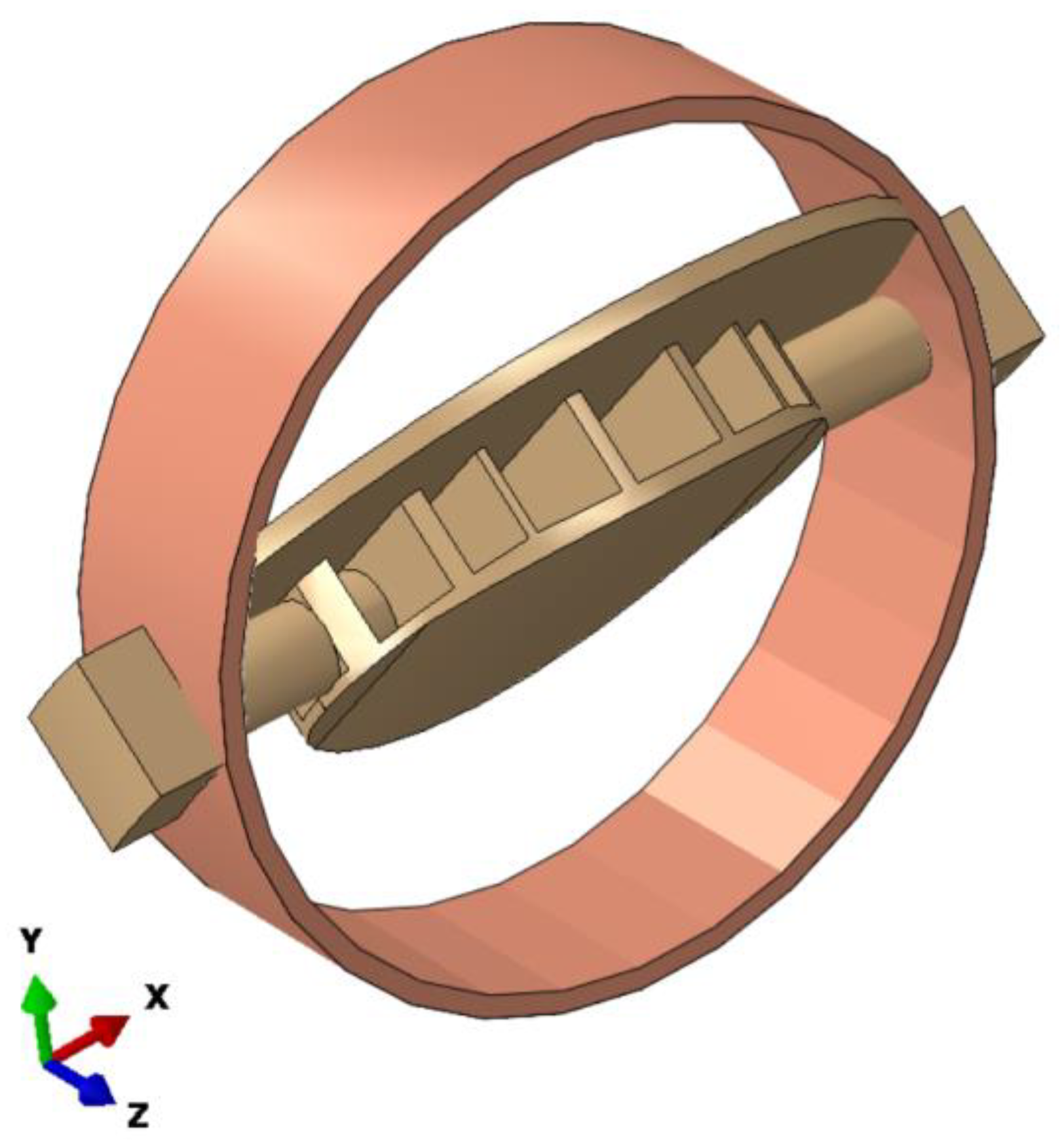
The level of detail that should be included in the finite element (FE) model is a crucial part of the cost analyses, as adding some components such as the valve gate disc is time-consuming and significantly increases the analysis cost and time. To this end, a model of the gate disc was created, as shown in Figure 5, and the model was analyzed including the gate disc. The findings indicated that incorporating such intricate details did not enhance the results; in fact, it substantially increased both the time required for preparation and analysis in comparison to omitting the disc from the model. The observed valve deflection when the gate disc was included in the model was 2.29 mm, while it measured 2.24 mm when the gate disc was excluded. Consequently, it was concluded not to model these highly detailed components due to the associated rise in computational expenses. However, the gate disc exists, and has weight, and its weight might affect the valve deflection. Therefore, the gate disc’s weight was approximated and employed a solid shaft (bearing housing with a gap between the bearing housing and the valve) that matched the gate’s weight for future models.

3.1.2. Mesh Sensitivity Analysis

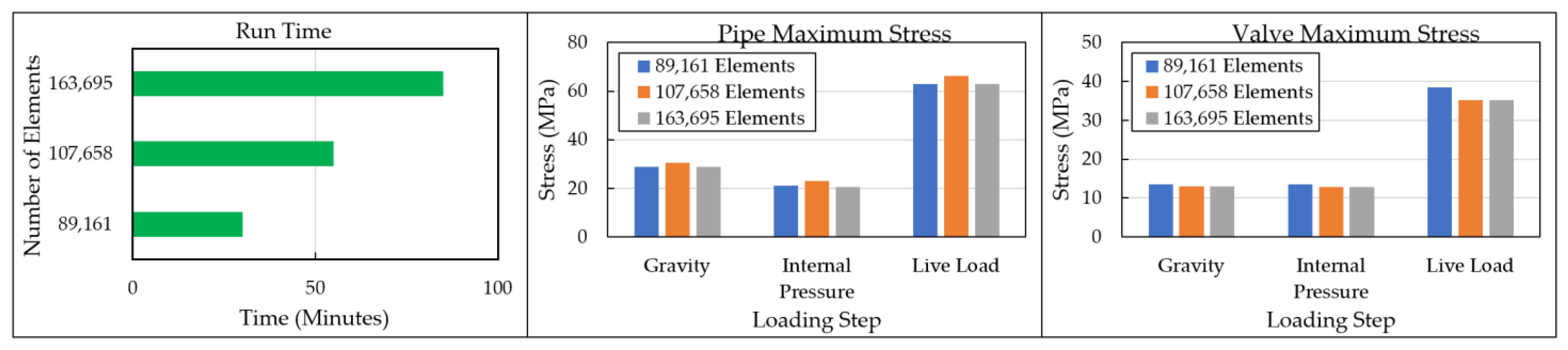
The last step in finalizing the benchmark model was to perform a mesh sensitivity analysis to ensure the accuracy of the results. Due to the size of the model, three different mesh sizes for different components were considered with a total number of elements of 89,161, 107,658, and 163,695. The stress results showed slight variations for both the valve and pipe. However, the run time of the analysis was significantly affected by increasing the number of elements. Figure 6 shows the data observed from the mesh sensitivity analysis. A small variance in the valve stress was observed, and the remaining variations were negligible. Therefore, the final selected total elements were 107,658 elements, and the size of each component has been discussed in the previous section. 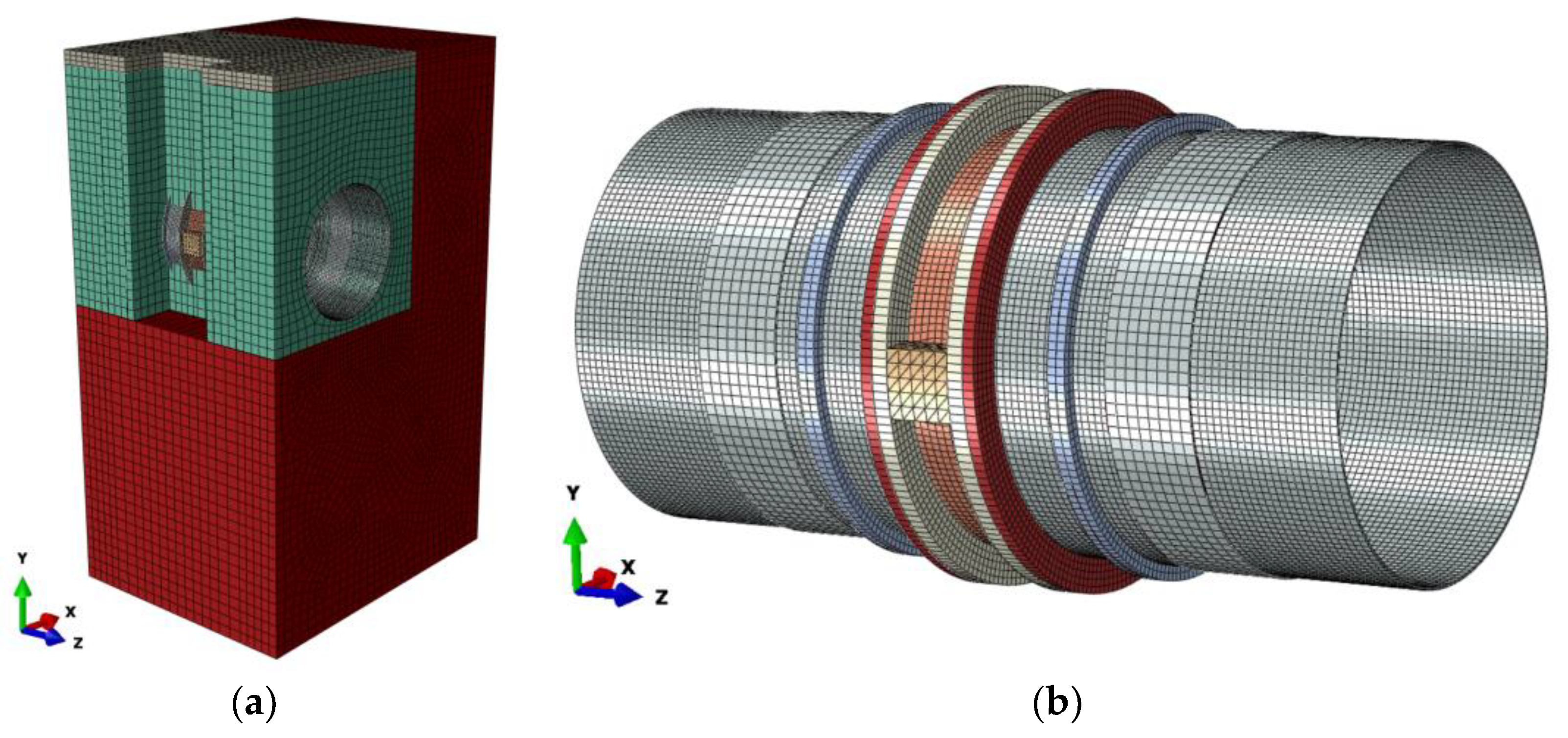Figure 7 shows the meshed components of the manhole and the pipe–valve system for the intermediate mesh size.

3.1.3. Final Selected Benchmark Model

The final selected FEM is shown in Figure 1 and Figure 2, including a 2.5 mm gap between the valve body and the BH to prevent unnecessary restraints. The gap was validated to be sufficient to prevent restraining effects by measuring the maximum valve deflection in the horizontal direction and comparing it to the remaining gap between the valve and the BH. The gap after deformation was measured to be less than 2.5 mm, indicating that the presence of the BH did not impede the deflection of the valve. By simulating the benchmark model as previously described, the component’s stresses were obtained. The maximum observed stresses were 52.3 MPa, 10.1 MPa, 67.6 MPa, and 48.1 MPa for the stiffening rings, butt straps, pipes, and valve, respectively. The focal point, in terms of stresses, is that the maximum observed stress at the bodies of the pipes and the valve should be less than the allowable stresses set by AWWA M11 [1] and AWWA C516 [4], respectively. The pipe’s allowable stress was specified by the AWWA [1] as “values of 50 percent of the specified minimum yield strength of the steel, not exceeding 18,000 psi (124 MPa) for the working pressure”. As specified by AWWA M11 [1], the steel pipe’s allowable stress was 125 MPa compared to the obtained steel stress of 67.6 MPa, indicating that the pipe stress was well below the allowable limit and that the design was safe. Moreover, AWWA C516 [4] specifies the allowable valve stress to be “the lesser of 1/5 of the tensile strength or 1/3 of the yield strength for alloy ductile iron, ductile iron, cast or fabricated steel, and stainless steel materials”. Therefore, the valve allowable stress is the lesser of $\frac{1}{3}\times 310=103$ MPa or $\frac{1}{5}\times 448=89.6$ MPa, and in this case the tensile strength of 448 MPa controls the allowable stress, which equals 89.6 MPa. When the obtained valve stress equal to 48.1 MPa was compared to the allowable stress, it was well below the allowable stress, and therefore both the pipe and the valve were designed safely. Finally, the deflection of the valve and the pipe is the second limitation of a large-diameter pipe–valve system, with the pipe deflection being 2–5% of its outer diameter, and the valve deflection being 1.5 mm under gravity.

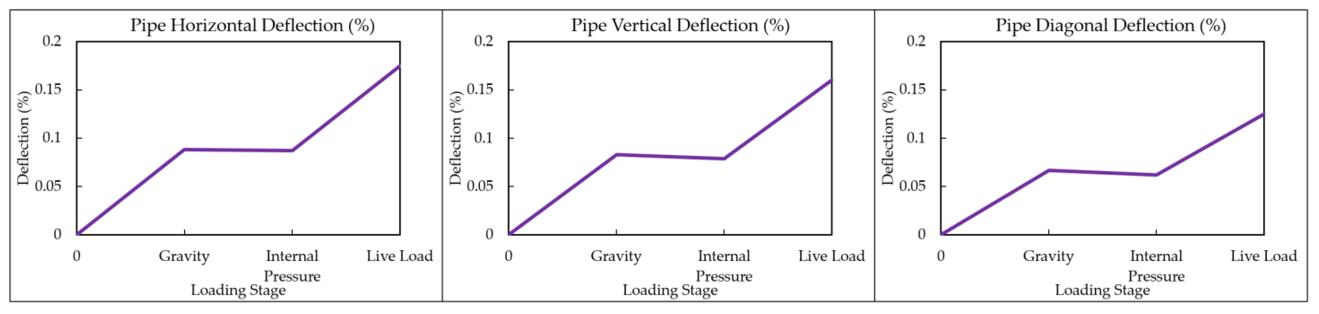
Figure 8 shows the pipe deflection percentage of its outer diameter. The results in all deflection directions showed that even after applying the extreme live load on the model the maximum observed pipe deflection was 0.175% of its outer diameter, which is way below the allowable deflection of 2%.

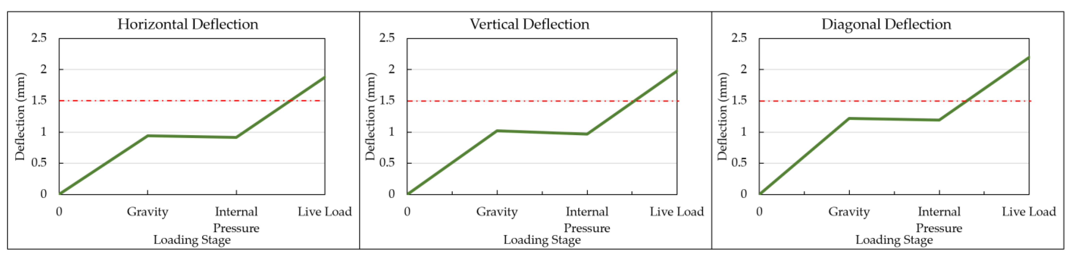
Figure 9 shows the obtained valve deflection. The results showed that under gravity, the valve deflection values were less than 1.5 mm (red dashed line in Figure 9). The maximum observed deflection was a 1.02 mm vertical deflection under gravity, which is less than the allowable deflection of 1.5 mm. Furthermore, the internal pressure was applied at the internal surfaces of the pipes and the valves, and it was applied in all directions. On the other hand, gravity is a vertical load distributed on the top half of the valves and the pipes. As a result, the internal pressure affects the pipes and the valves in the opposite direction of gravity. Therefore, the internal pressure would reduce the deflection of the pipes and the valve. This is known as re-rounding effects.

To validate the stress results obtained in the FEA, the modified Iowa formula to predict pipe deflection can be employed, as indicated in AWWA M11 [1]. It is worth mentioning that this formula provides an estimate of the horizontal deflection of the pipe under earth loads. Therefore, it can predict pipe deflection under gravity and live loads without internal pressure. Hence, the modified Iowa formula was used to predict the pipe deflection at a distance away from the interaction and BC regions under gravity, and the results were compared to those obtained in the FEA. Furthermore, the formula was only established in the foot-pound-second (FPS) system of units. Therefore, the data shown below are in the FPS system of units, and the predicted deflection value was converted to the international system of units (SI). The modified Iowa formula is shown in Equation (1):

$$∆x=D_l\frac{KW{r}^3}{EI+0.061E^{\prime }{r}^3}$$

(1)

where $∆x$ is the predicted horizontal deflection (mm), $D_l$ is the deflection lag factor (1.0), K is the bedding constant (0.1), W is the load per unit of pipe length (lb/lin in.), which can be calculated in Equation (2), r is the mean radius of the pipe (in.), $E^{\prime }$ is the modulus of soil reaction of embedment material, E is the modulus of elasticity (psi), I is the transverse moment of inertia per unit length of individual pipe wall equal to ($\frac{t^3}{12}) ({\mathrm{i}\mathrm{n}.}^3)$, and t is the pipe wall thickness (in.). Equation (2) is as follows:

$$W=\raisebox{1ex}{$W_c$}\!\left/ \!\raisebox{-1ex}{$12$}\right.+\raisebox{1ex}{$W_L{D}_c$}\!\left/ \!\raisebox{-1ex}{$144$}\right.$$

(2)

where $W_c$ is the prism load (dead load on the conduit) (lb/lin ft of the pipe) given in Equation (3), $W_L$ denotes the extreme external loading, such as railroads and heavy construction equipment, and $D_c$ is the outer diameter of the pipe (ft). Equation (3) is as follows:

$$W_c=\omega H_c\frac{D_c}{12}$$

(3)

where $\omega$ is the unit weight of fill (lb/ft³), and $H_c$ is the height of the fill above the top of the pipe (ft). With the given data, as described in Section 2, the CLSM reaction modulus was between 3000 psi (21 MPa) and 25,000 psi (172 MPa) [1]. As the actual value of E′ (which is not an inherent material property and cannot be directly quantified) is usually determined indirectly through deflection measurements (as outlined in AWWA M11), the calculations for pipe deflection will involve using both upper and lower estimates for E′. The predicted pipe’s horizontal deflection was 0.367% and 0.045% of the pipe’s outer diameter based on the lower and upper E′ values, respectively. When comparing the pipe’s maximum horizontal deflection under gravity obtained in the FEA of 0.088%, the result of the FEA falls within the range of the predicted pipe deflection and can be considered acceptable. However, using the upper and lower limits of E′ may result in an overestimation or underestimation of the pipe/valve deflection. Hence, non-linear 3-dimensional finite element analysis of such systems is necessary for predicting pipe–valve deflections.

3.2. CLSM vs. Regular Backfill Material Effects on the Pipe and Valve Deflections

After finalizing the benchmark model, the first evaluation compares the deflection of the pipe and the valve under different backfill materials. With the same configurations and settings discussed in Section 2, the FEA model was used with varying CLSM properties to regular backfill soil using the Mohr–Coulomb plasticity material model. The backfill soil has a unit weight of 1762 kg/m³, modulus of elasticity (E) of 48.3 MPa, and a Poisson’s ratio of 0.35, and its Mohr–Coulomb plasticity parameters include an angle of friction of 48^o, dilation angle of 7^o, and 0.1 MPa cohesion.

Table 6. Valve deflection comparison between using different backfill material.

Deflection	Loading Step	CLSM Backfill	Soil Backfill
Horizontal deflection (mm)	Gravity	0.940	0.889
	Internal pressure	0.914	0.889
	Live load	1.880	1.800
Vertical deflection (mm)	Gravity	1.020	0.940
	Internal pressure	0.965	0.900
	Live load	1.980	1.950
Diagonal deflection (mm)	Gravity	1.220	1.160
	Internal pressure	1.190	1.020
	Live load	2.200	2.168

compares the valve deflection between using CLSM and regular soil as backfill material.

The results show that the valve deflection was not significantly affected by changing the backfill material to soil; this was due to the high friction angle and unit weight of soil being close to that of CLSM.

3.3. Internal Pressure and Live Load Limits

In this section, the internal pressure and live load limits before the valve deflection exceeds the allowable limit are investigated. To this end, two different models were analyzed, wherein the first model had its internal pressure gradually raised from 0.1 MPa to 1.73 MPa and a 0.1 MPa live load applied after that. Thereafter, the second model experienced a gradual increase in live load from 0.055 MPa to 0.14 MPa, while maintaining a constant internal pressure of 0.1 MPa. 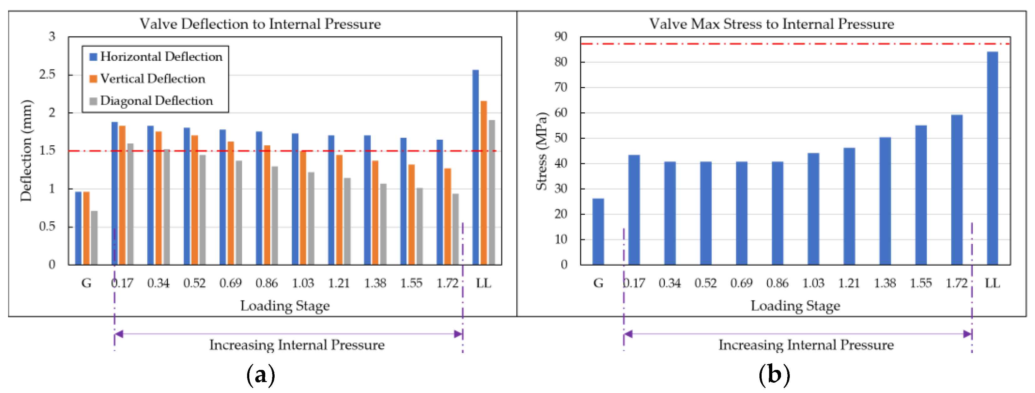Figure 10 illustrates the valve’s deflection and stress evolution as the internal pressure increases, indicating that valve deflection decreases as internal pressure increases. Furthermore, the maximum valve stress due to internal pressure was found to be 59.2 MPa, which remains below the allowable limit of 89.6 MPa. However, once the live load was applied, the valve stress reached the allowable limit of 89.6 MPa. Consequently, the pipe–valve system can endure an internal pressure of 1.73 MPa without surpassing the allowable stress thresholds. 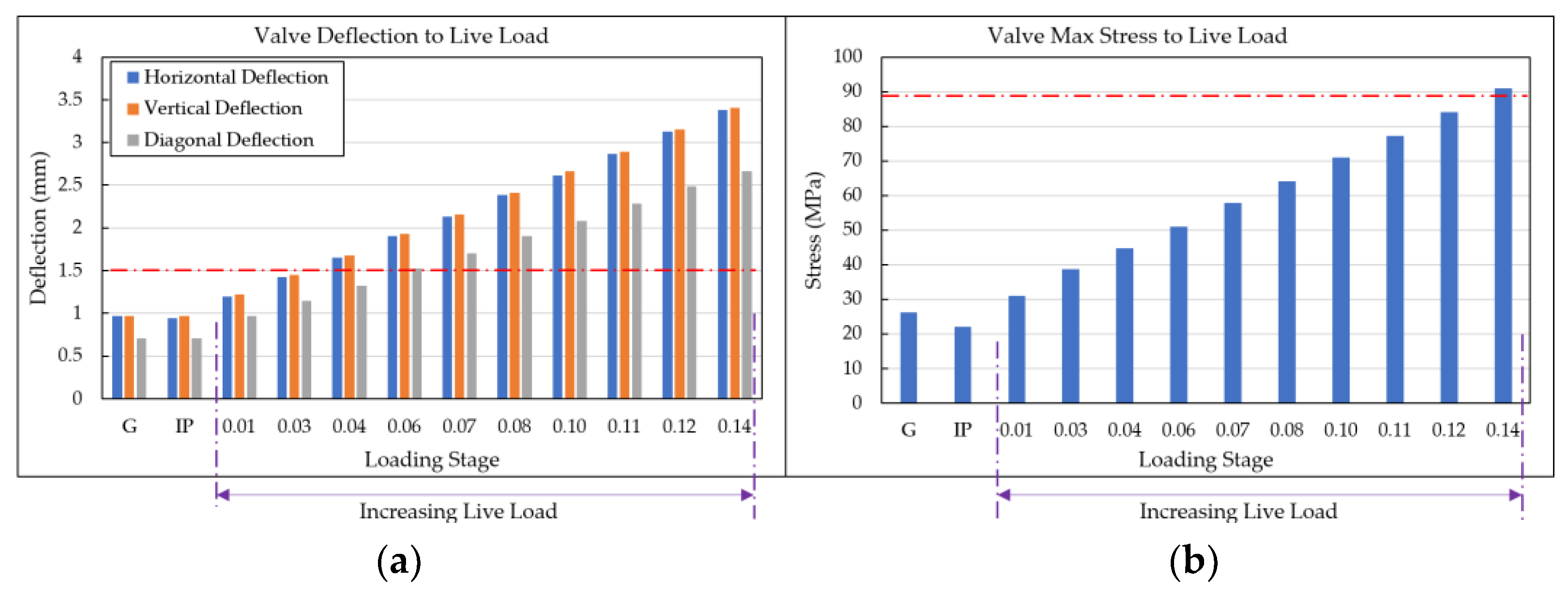Figure 11 demonstrates the development of valve deflection in response to an increase in live load.

The pipe–valve system can endure an applied live load of around 0.041 MPa at 2438.4 mm from the top of the topsoil to the pipe crown. However, once the live load surpasses 0.041 MPa, the valve deflection surpasses the permitted deflection threshold of 1.5 mm, which is indicated by the red dashed line in Figure 11. It should be noted this is just a theoretical value, since the 1.5 mm limit does not apply to the deflection under live load. Additionally, the stress exceeded the allowable stress limit when the applied live load reached 0.14 MPa.

3.4. CLSM Modulus of Elasticity Effects on Valve Deflection

Controlled low-strength material (CLSM) plays a pivotal role in controlling deflection within the pipe–valve system. It serves as a substitute for traditional granular backfill, effectively mitigating deflection concerns. The CLSM modulus of elasticity can be as low as 41 MPa and as high as 518 MPa. The CLSM is known in the industry as “Slurry”, in other words, bad concrete made with soil, cement, and water. The CLSM modulus of elasticity can be obtained using field experiments and there is no available field data to calibrate the CLSM properties in the FEA. It varies based on site conditions (temperature, type of soil, time of testing, etc.). Therefore, a comprehensive parametric investigation, in this context, is necessary. A cursory review of pertinent literature sources [16,17,18,19] reported higher CLSM modulus of elasticity values than the value used in this study, as the selected value represents the lower limit and is generally associated with the modulus of elasticity during the early stages of curing. The value selected in this study was adopted from Takou [20], which was carried out on the same project. 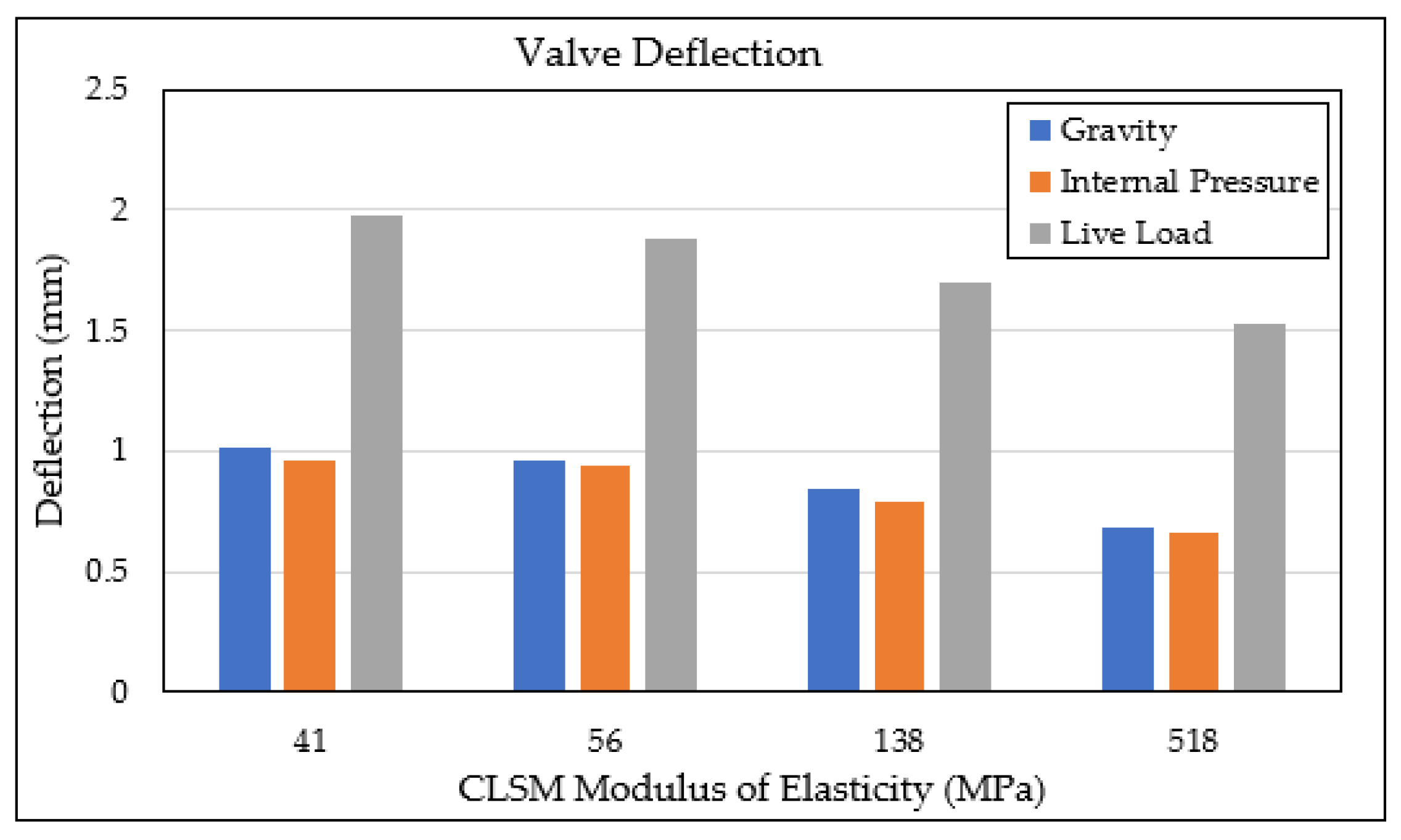Figure 12 visually illustrates the relationship between the CLSM modulus of elasticity and valve deflection. The results unequivocally demonstrate that as the modulus of elasticity increases, deflection decreases—a trend in line with expectations.

Expanding on this topic, it is crucial to conduct a more extensive study to precisely determine the optimal modulus of elasticity for the CLSM in the pipe–valve system. This investigation should encompass various curing stages and consider a broader range of factors that may influence deflection behavior. Such a comprehensive approach will facilitate more accurate deflection control and enhance the overall performance and reliability of the pipe–valve system.

3.5. Soil Compaction Application

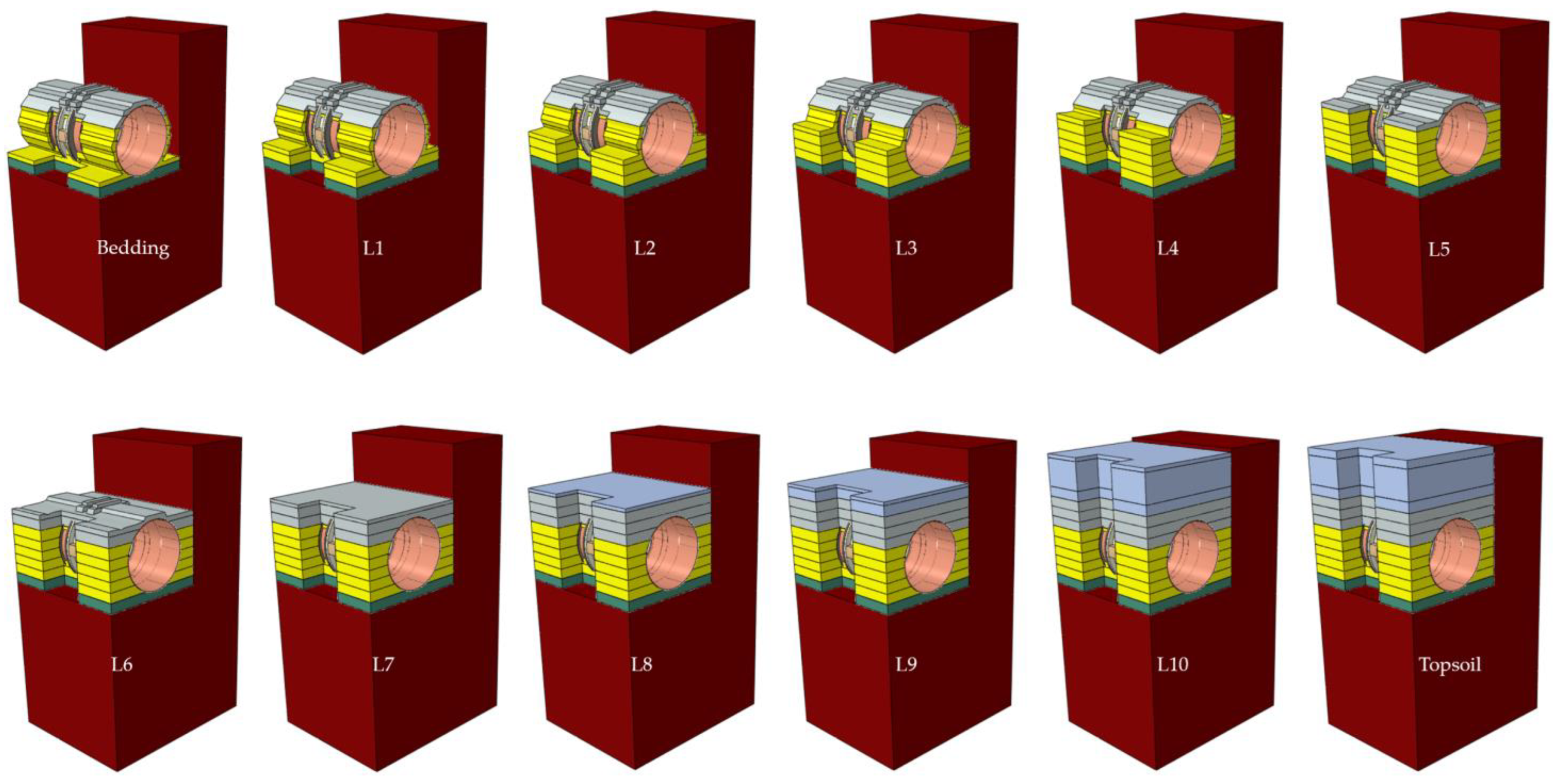
Soil compaction has been recognized as a substantial factor affecting the deflection of large-diameter pipes and valves and, consequently, the overall performance of the pipe–valve system. Consequently, it is essential to anticipate how this system will respond to compaction during backfilling if conventional backfill is used. However, it is important to note that this scenario is theoretical, since in real-world applications the pipe–valve system is backfilled using CLSM without undergoing any compaction processes. In this section, the pipe–valve system was modeled and simulated under compaction settings. To this end, bedding, five layers of embedment, two layers of regular backfill, three layers of select-fill, and finally regular backfill soil were considered on the top of the pipe–valve system. Figure 13 shows the modeled layers used to apply compaction on the pipe–valve system. The first step involved the placement of bedding material and constituting layer 1. Subsequently, additional layers were sequentially added, each accompanied by its own specific weight and compaction process. Compaction application was adopted from the literature [10,21]. Thereafter, internal pressure and live load were subsequentially applied to the system. Layers 1 through 9 had a 406.4 mm thickness, and the thicknesses of layers 10 and 11 were increased to 1143 mm to reduce the analysis cost.

In real-life scenarios for the compaction of buried pipes, the maximum layer thickness should not be more than 457.2 mm for the pipe–valve to obtain a uniform compaction throughout the layer. However, layers 9, 10, and 11, and the topsoil are far enough above the top of the pipe, and applying compaction will not affect the pipe–valve deflections.

Table 7. Material properties of the backfill materials used in compaction application.

Layer	Material	E (MPa)	C (kPa)	ϕ (°)
Bedding	Gravel	10.3	13.8	45
L1–L5	Pea gravel	21.4	13.8	34
L6–L8	Select fill	9.70	13.8	24
L9–topsoil	Clay soil	4.80	96.5	8

shows the material properties used for each layer. The application of a compaction load results in added stress within each layer, leading to expansion in the X-direction (towards the pipe–valve system). To simulate this expansion, an approximate approach was employed, as elaborated in Emami Saleh et al. [10]. This method assumed a hypothetical thermal expansion coefficient of 0.0005 and factored in the stress induced via an embedment wheel using a fictitious thermal expansion model. Specifically, it was assumed that compaction was carried out using an embedment wheel with a weight of 3629 kg, and that it could be applied at a minimum distance of 152.4 mm from the pipe–valve system. The stress generated via the wheel at the center of each layer was then determined using the methodology outlined in Abolmaali et al. [12]. Subsequently, this stress was converted into a change in temperature using the fictitious expansion coefficient and the modulus of elasticity, as described in [10,12].

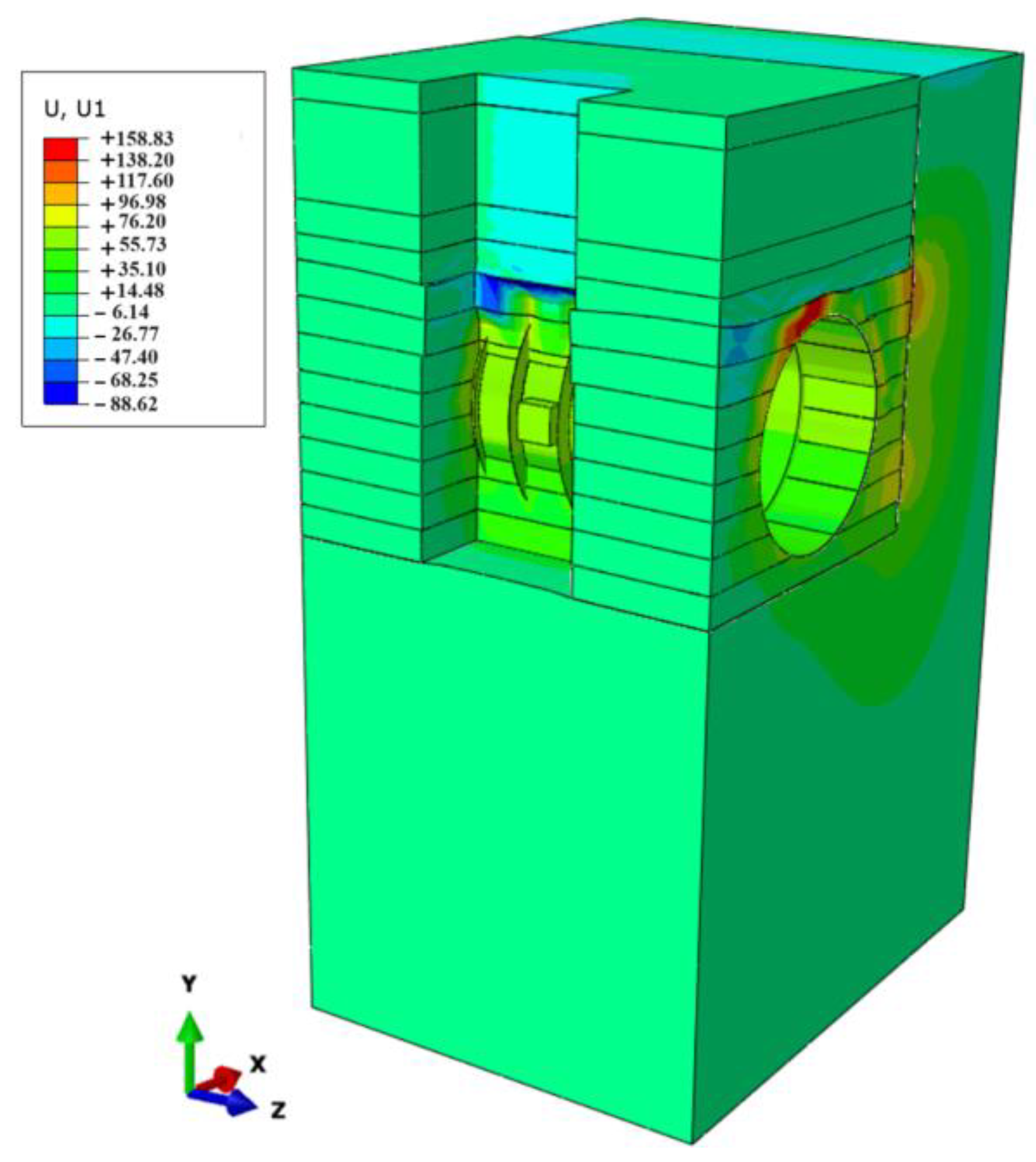
The results showed that the constraint applied at the negative X-direction caused restraining effects on the layers, preventing it from expanding (as if it was free) as expected, as shown in Figure 14.

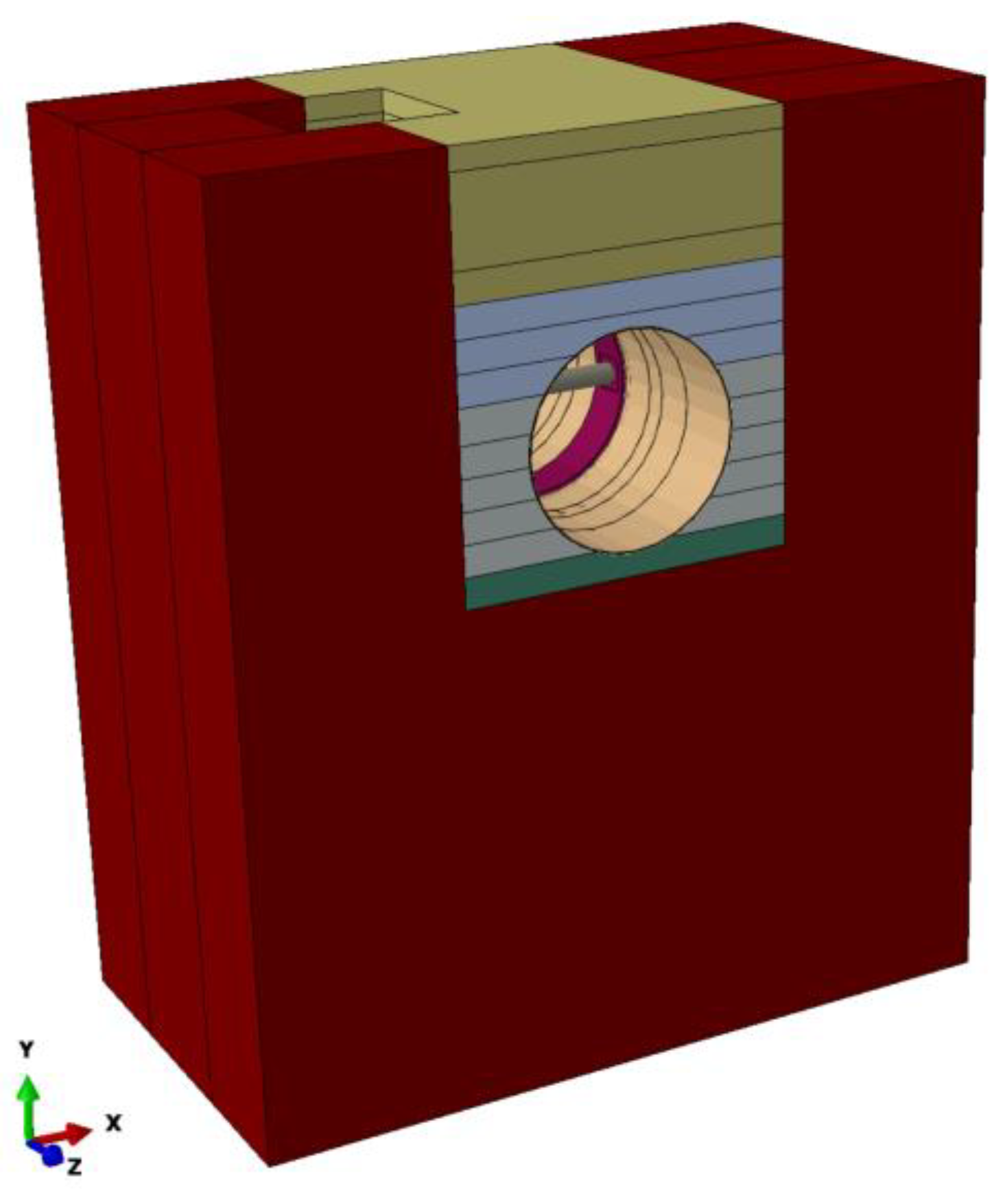
As can be seen in Figure 14, the vertical surface of the backfill soil prevents the expansion of soil due to compaction, which, in turn, affects the pipe–valve system deflection. Therefore, such a model is not realistic, and the whole manhole must be modeled to achieve realistic results. Hence, as shown in Figure 15, the whole depth of the manhole has to be modeled, and only the outermost vertical surfaces of the native soil have been restrained in the perpendicular direction to the surface; the mesh, materials, and pipe–valve system are the same as discussed previously. Compaction has been applied similarly with the same number of layers.

The results showed that the valve deflection under compaction was 1.73 mm, 1.53 mm, and 1.30 mm for the horizontal, vertical, and diagonal deflections, respectively. As expected, since the compaction affects the valve horizontally, the valve’s horizontal deflection experienced the most impact, and the deflection of the valve exceeded the allowable limit of 1.50 mm under gravity alone. This is one of the main reasons for which CLSM is used as an alternative material to soil, since it does not require compaction.

Finally, the effect of native soil strength on the deflection behavior of pipe–valve systems subjected to compaction was investigated and found to be a pivotal and noteworthy factor. The extent of valve deflection exhibits substantial variability contingent upon the inherent characteristics of the native soil. Specifically, when the native soil is characterized by a high level of stiffness, denoting a significant modulus of elasticity, the valve horizontal deflection under gravity alone can increase considerably, potentially reaching up to 2.14 mm. Conversely, in scenarios where the native soil possesses a notably low modulus of elasticity, the valve deflection experiences a remarkable reduction, plummeting to as low as 0.90 mm under the same conditions. This contrast in deflection behavior is intrinsically linked to the mechanical properties of the native soil. The importance of comprehending this relationship between native soil attributes and valve deflection cannot be overstated. In practical terms, native soil with a high modulus of elasticity results in resistance to deformation. Consequently, when compaction is applied, combined with live loads and internal pressure, the pipe–valve system experiences more deflections. Conversely, soils characterized by a lower modulus of elasticity offer greater flexibility, thereby constraining the extent of valve deflection under comparable conditions. 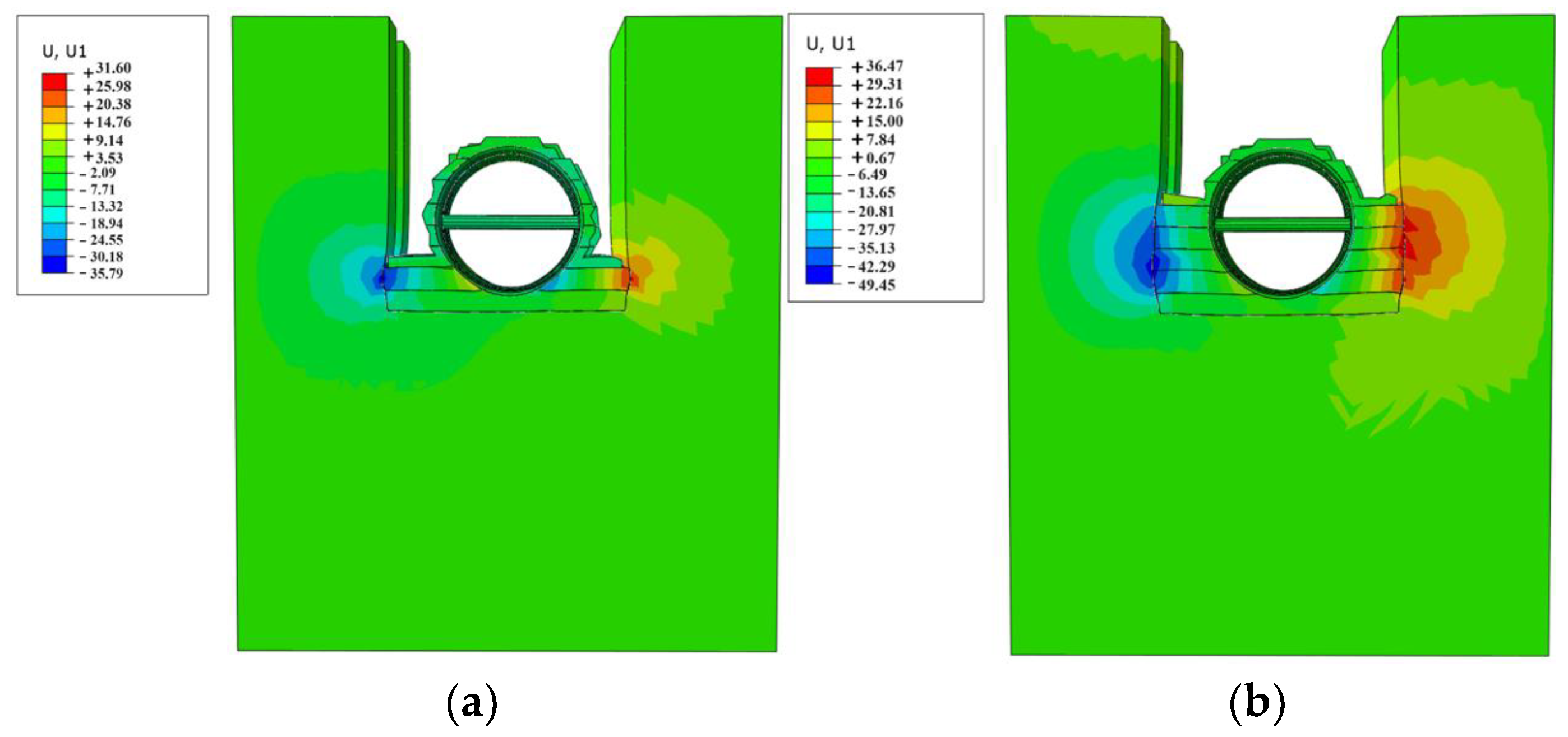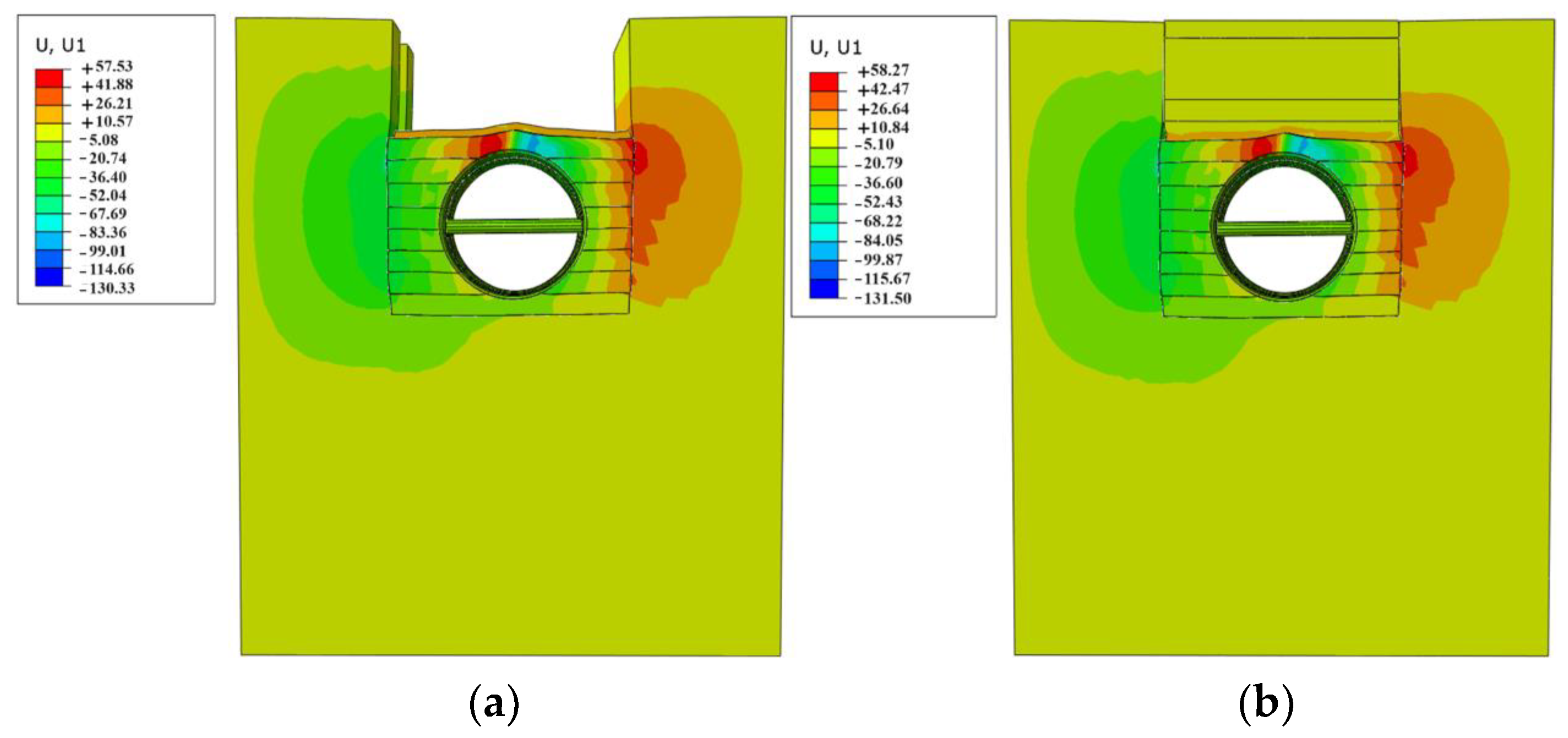Figure 16 shows the deformed shape of the pipe–valve system after applying compaction to layers 2 and 5, and Figure 17 shows the deformed shape of the pipe–valve system after applying layer 8 and the topsoil. Since layers 9 up to topsoil are high above the pipe crown, no compaction was applied, as it will have no effect on the pipe and only the weight of the layers is taking place (vertical direction). Therefore, the contours shown in Figure 17a,b may seem identical.

It is worth mentioning that in Figure 16 and Figure 17, the displacement contours on the figures are four times magnified for better visualization.

4. Summary and Conclusions

This article addressed some of the concerns of the industry about direct-bury large-diameter pipe-butterfly valve systems. It provided a method to find the deflection of the pipe and the valve under operational conditions to avoid potential issues using FEA to test pipes and valve designs before site installation. Three-dimensional non-linear FEAs have been conducted considering the effects of different conditions that may affect the valve deflection. Based on the results obtained in this study, the following can be concluded:

• A smaller mesh in FEA is not always the best choice; as discussed in this paper, an intermediate mesh was used.
• Not all components of the FEA model are necessary to achieve a realistic result, such as the case with the valve gate disc. Some components can be converted into simpler geometries that can save a substantial amount of time and analysis cost.
• Internal pressure and live load capacities can be predicted using FEA by ramping up their values until the model fails based on the relevant acceptance criteria. This can be a great method to evaluate and compare theoretical results with the required design.
• Valve deflection is inversely proportional to the CLSM modulus of elasticity. A higher CLSM modulus of elasticity resulted in less deflection.
• Native soil strength plays a significant role in pipe–valve system deflection when soil compaction is applied. Higher-strength native soil causes higher deflections.
• When compaction is considered, the whole manhole must be modeled to obtain accurate results, while in the absence of compaction (use of CLSM) modeling half of the manhole is sufficient for the analyses.

Finally, the authors would like to highlight the necessity to investigate the geometrical properties of stiffeners to evaluate their effects. It is also recommended to set benchmarks for large-diameter pipe–valve systems under extreme weather conditions, such as freezing, develop machine learning algorithms to automate the FEA modeling, and to develop the design equations.