Supply-Driven Analysis for a Continuous Water Supply Network Based on a Pressure-Based Outflow at the House Outlets under Peak Withdrawal Scenarios

Abstract

This research brings a new analysis method for a continuous water supply distribution network. The number of house service connections in different story buildings, rather than the nodal peak demand, shall be accounted for in the analysis. This work aims to consider the flow when pipes are opened in the house plumbing systems. The approach deviates from a traditional peak demand-based analysis of the water distribution network. The analysis gives the flow rate at each nodal point that could be observed in the different story buildings. The methodology is applied to a hypothetical network and shows how much flow and nodal pressure can occur when different percentages of consumers are in an active state. This study indicates that the peak demand-based sizing of the supply pipes could have a deficient capacity under real scenarios. The proposed analysis method will help to understand the actual behavior of the network.

1. Introduction

The simulation of water distribution networks (WDNs) is performed in three ways for selected network geometry and hydraulic properties. They are demand-driven, pressure-driven, and volume-driven. The demand-driven analysis (DDA) results are valid if no pressure deficiency exists at the nodes. Pressure-driven analysis (PDA) can compute the pressure-dependent outflow for a designated minimum-maximum pressure range. Volume-driven analysis (VDA) computes the volume of water that could be supplied upon expected demand. Analysis based on these three approaches shall be required to better design WDNs and to understand the network behaviors when it is servicing under component failures and a shortfall in source water availability. Computational fluid dynamic (CFD) methods are commonly used in the assessment of hydrodynamic phenomena in pipes and connections [1].

The peak nodal demand is the main parameter for pipe sizing using DDA. The peak demand is calculated based on the forecasted population that needs to be served during peak water usage. The peak hourly demand is usually between 1.3 and 3.0 times the average hourly demand [2]. The entire design process is carried out using peak hourly demand. The volume of water required over a day is calculated based on per capita water usage. Its value varies from place to place, and different values are used for rural and urban communities. The analysis of domestic water consumption indicates 92 L/person/day for healthy urban lifestyles with restrictions on everyday activities and 175 L/person/day for unrestricted water usage. It is quantified according to estimated needs; the consumption rate is estimated as 227 L/person/day, and the ultimate level of consumption happens at the rate of 314 L/person/day [3]. The peak demand occurs between 6.00 a.m. and 7.00 a.m. and between 5.00 p.m. and 7.00 p.m. [4]. Residential water demand has shown high variability due to variations in water fixtures and appliances coupled with different routines and timing of withdrawal by the end users [5]. During peak time, water withdrawal may happen simultaneously from several fixtures. The flow from these fixtures occurs based on the pressure in the street main pipeline. The more pressure availability, the more volume will be delivered quickly, and vice versa. Hence, the pressure-dependent outflow from the fixtures at peak usage shall be accounted for in modelling. In the case of a flat terrain, the houses located near the source derive more benefits due to the availability of more pressure, whereas the houses located far away from the source are deprived of pressure, and less supply is possible. Due to these aspects, the simulation that considers the actual flow to the houses could provide a better analysis regarding meeting the demand, especially at peak times. An estimate of total outflow at peak usage of water shall be carried out, and the same shall be used in the analysis of WDN. This could provide valuable information on the pressure at several nodes and make it easier to manage pressure better. In the DDA and PDA, the demand for each node shall be set and analyzed. In VDA, the volume of water to be supplied at each node shall be set through outlet sizing storage at the outlet. The VDA is the most suitable method of analysis for intermittent water supply (IWS) systems, where water is collected in the underground storage system during supply hours [6]. In the continuous water supply (CWS) system, maintaining service pressure at peak hours is very important to meet the volume of water expected by consumers. In the present study, a new approach is formulated to simulate the network based on the number of fixtures kept open during peak hours in each house. The proposed approach analyzes the network based on the number of house service connections (HSCs) provided and the number of plumbing fixtures simultaneously active during peak hours. The analysis can be easily performed once the number of HSC incident to every node is known. The flow rate at each house at peak hours can be directly ascertained using this approach. The supply at each fixture happens only based on the available pressure, and the analysis procedure is named supply-driven analysis (SDA). The SDA can be implemented using the Emitter option available in the EPANET. This paper further presents a method for calculating the emitter coefficient under different scenarios.

2. Pressure Flow Relationship for House Service Lines

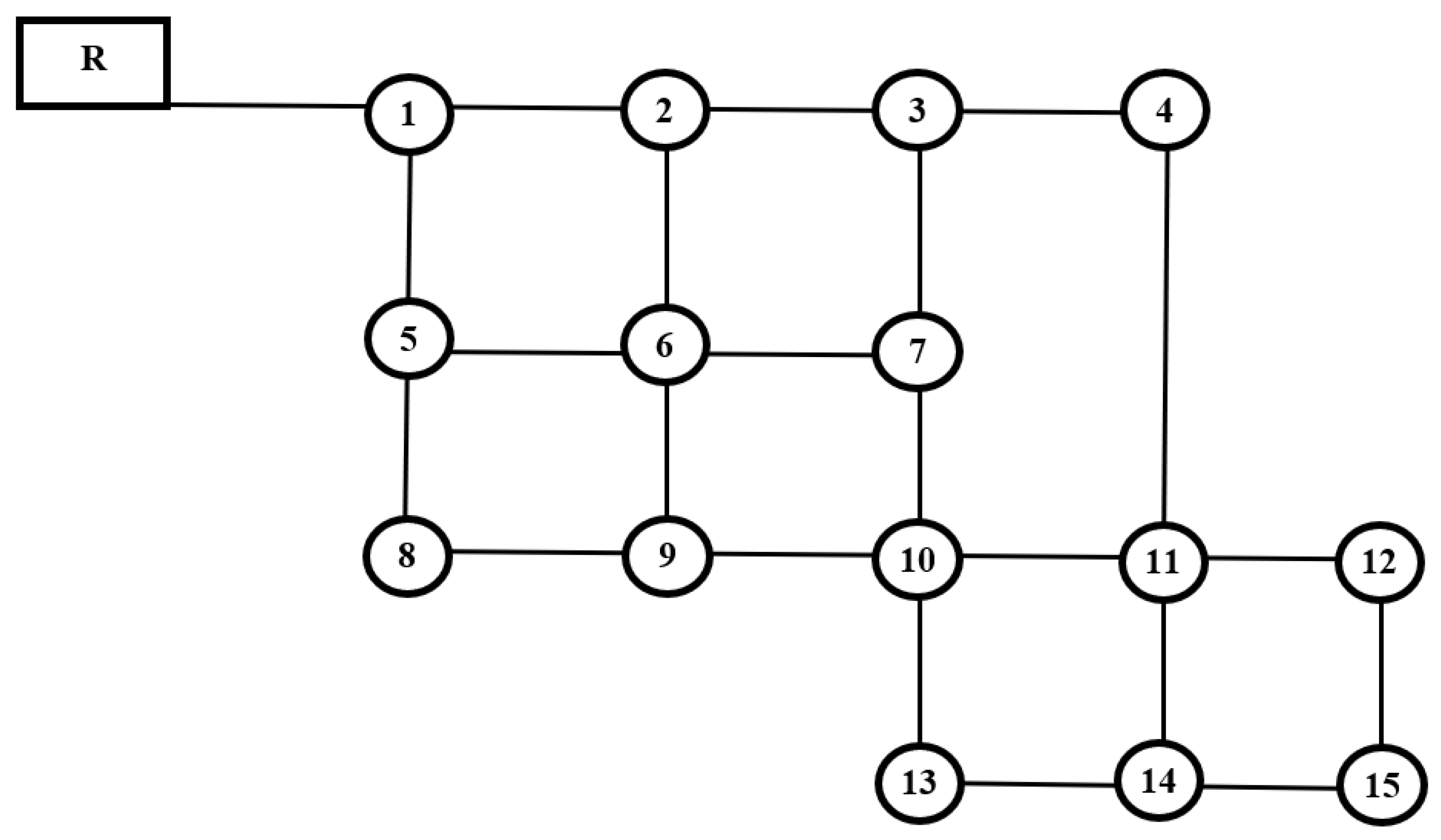
In a CWS system that directly connects with a house plumbing system (Figure 1), the flow rate for each HSC can be estimated using the arrangement shown in Figure 2. The outflow from the house plumbing system depends on the availability of pressure. Each house can have several outlets, like a water tap in the kitchen, a washing machine supply, a bathroom water shower, and a cistern flush in the lavatory. Simultaneous supply from all outlets provides the maximum possible withdrawal. It is to be noted that supply from these outlets is based on the available pressure. Hence, satisfying the required demand is related to time. There could be more than four fixtures in a house. Considering the worst scenario where five fixtures are opened simultaneously, this could be considered as peak demand. This peak demand can be estimated by considering the network between the connection at the main supply and any of the five plumbing fixtures of the house. The available static pressure in the water main in the street pushes the water to the service line based on the pressure available.

A house service pipeline connecting the house’s internal pipe network can be treated as a separate system that can be simulated for various static pressures to obtain the relationship between pressure and supply. The prepared network layout consists of a reservoir that provides a static pressure head to the system, and a pipeline connecting the municipal main pipeline with the service line. The diameter of this pipeline can be taken as either 25 mm or 18 mm, and the diameter of the internal pipeline can be considered as either 18 mm or 12 mm. The diameter can be decided based on local practice. The minor loss coefficient for the service line can be taken as 1.8 [7]. The selection of house service pipe diameter and internal house pipe diameter can also be taken as actual values adopted in the respective region in the analysis. In the present work, a 18 mm diameter is considered for house service connections and a 12 mm diameter for raising pipes and internal pipes for single-story buildings (ground floor alone). In the case of two- and three-story buildings, 25 mm, 18 mm, and 12 mm diameters are considered for house service, raising, and internal pipes, respectively. The pipe network layout for a single-story building shown in Figure 2 is considered for the present study. The length of the house service pipeline and internal pipelines may vary from house to house. Hence, a reasonable length can be considered for the analysis. Usually, the plumbing fixture outlet level would have been positioned at different levels based on convenience and the ceiling height of the building. An average height of 1.5 m from the floor level is considered to obtain the flow vs. pressure head relationship.

Table 1. Network details for the single-story house.

Reservoir/Node	Elevation (m)	Pipe Number	Length (m)	Diameter (mm)
R	Variable (5 m to 30 m)	1	1.00	18
R1	3.0	2	4.00	18
R2	3.0	3	2.00	18
R3	3.0	4	2.00	12
R4	3.0	5	3.00	12
R5	3.0	6	3.00	12
1	0.0	7	3.00	12
2	0.0	8	3.00	12
3	1.5	9	3.00	12
4	1.5	10	3.00	12
5	1.5	11	3.00	12
6	1.5	12	3.00	12

gives the network details for a single-story building. The Hazen–Williams head loss equation is used, and the roughness coefficient for all pipes is taken as 130 for the network analysis. The static pressure will be provided by the source reservoir (R), which mimics the availability of static pressure in the pipeline. Water delivery at various outlets can be computed by connecting a reservoir at the respective outlets (R1 to R5). A minor loss coefficient of 1.8 is fixed to all pipes to account for losses due to bends, contractions, and fixtures. Two scenarios are considered to establish the relationship between supply and pressure head. In the first scenario, a maximum of five fixtures are considered to be active at peak time for all three types of buildings. In the second scenario, two fixtures are kept active for all three types of buildings. Through simulation with different static source pressure heads, the total supply for each house type is obtained. The EPANET 2.2 software [8] is used to analyze the network.

In the analysis, each pipe-connecting fixture (artificial reservoir) is provided with a check valve to prevent reverse flow in the pipeline. A plot is prepared between the flow and pressure head for all scenarios. The relationship between flow and pressure head is obtained as a power equation in MS Excel.

Table 2. Relationship between supply and pressure.

Type of Building	Number of Fixtures in Active State	Flow (Q) vs. Pressure Head (P) Relationship	R2 Value	Correction Coefficient (Cc)	Adjusted Q vs. P Relationship
Single-story	5	$Q=6.024P^{0.611}$	0.9987	0.971	$Q={5.849P}^{0.62}$
Double-story	5	$Q=14.129P^{0.669}$	0.9955	1.176	$Q=16.616P^{0.62}$
Triple-story	5	$Q=15.287P^{0.670}$	0.9968	1.180	$Q=18.039P^{0.62}$
Single-story	2	$Q=5.206P^{0.612}$	0.9987	0.974	$Q=5.071P^{0.62}$
Double-story	2	$Q=10.775P^{0.671}$	0.9957	1.184	$Q=12.758P^{0.62}$
Triple-story	2	$Q=13.049P^{0.668}$	0.9975	1.172	$Q=15.293P^{0.62}$

gives the equations for various scenarios obtained from the generated data. These equations are in the form of KPⁿ and are akin to the emitter equation used in EPANET (version 2.2) simulation software, in which K and n are the emitter coefficient and exponent, respectively. It is to be noted here that the obtained equations have different values of K and n. The K value for each node and each category of buildings can be set directly in the EPANET software, whatever the values. But no option is available to set a different value of n for each node. The software accepts one n for all nodes if the emitter option is activated for the simulation. To have a common exponent for double- and triple-story buildings, the emitter coefficient value for each case is corrected by multiplying with the correction coefficient as given in Table 2. The common n value corresponds to the single-story building when all five fixtures in the active state were used for all scenarios. Since there are three categories of buildings, it is not possible to set three K values for a node. Further, the emitter continues to be active when the node faces a negative pressure value during simulation. Under this circumstance, the emitter behaves as a source rather than a sink. To eliminate this situation and to handle three categories of buildings for supply, three small pipes of a 300 mm diameter, 0.1 m length, and roughness coefficient of 130 are connected with the demand node and with a dummy node at the other end, and a check valve is enabled for these artificial pipes (Figure 3). Now, in the fictitious nodes, emitter coefficients corresponding to single, double and triple stories are assigned. The elevation of all fictitious nodes shall be the actual demand node. No demand value shall be set to any nodes for this analysis. The network can be simulated after inputting the necessary data, as mentioned above. This basically requires the addition of a fictitious system to all nodes. Developments in hardware and software that are happening in the computing world have allowed to include all kinds of water supply information in modelling [9]. As the software is designed to handle more nodes and pipes for hydraulic analysis, the proposed approach can easily be adapted for any network size.

3. Hypothetical Network Preparation

A hypothetical network (Figure 4) is prepared to illustrate the proposed method of analysis of WDN. The network is supplied by one reservoir with a total head of 50 m. There are 15 demand nodes and 22 pipes. The elevation of all nodes is taken as 0 m. The geometrical properties of the network are presented in

Table 3. Hypothetical network details.

Pipe ID	Connecting Nodes	Length (m)	Pipe Diameter in mm	Number of Buildings in Each Type
				Single Story	Double Story	Triple Story
1	R–1	50	250
2	1–2	360	150	30	20	10
3	2–3	720	150	80	30	10
4	3–4	360	100	20	15	5
5	1–5	240	200	25	15	0
6	2–6	240	50	35	20	5
7	3–7	240	50	28	12	0
8	4–11	540	100	52	28	10
9	5–6	360	150	38	14	8
10	6–7	720	150	86	24	10
11	5–8	300	100	24	22	4
12	6–9	300	50	22	22	6
13	7–10	300	150	40	10	0
14	10–11	360	150	30	20	10
15	11–12	480	100	20	35	5
16	10–13	600	100	70	45	5
17	11–14	600	100	70	25	5
18	12–15	600	100	54	16	10
19	13–14	360	50	75	20	5
20	14–15	480	50	75	25	0
21	8–9	360	100	50	5	5
22	9–10	720	100	52	18	10

. The number of houses based on each type of story is assigned for each street, and then it is transferred to the end nodes of the pipe by taking half of the house service connections of each link.

Table 4. Node-wise building type and nodal demand.

Node ID	Node-Wise Single-Story Building	Node-Wise Double-Story Building	Node-Wise Triple-Story Building	Calculated Demand for PF = 3 (LPM)
1	28	17	5	104
2	73	35	13	252
3	64	29	7	208
4	36	21	8	136
5	43	26	6	156
6	90	40	15	302
7	77	23	5	219
8	37	13	5	115
9	62	23	10	198
10	96	46	13	323
11	86	53	15	321
12	37	26	8	148
13	72	33	5	229
14	110	35	4	310
15	65	21	5	190

provides node-wise house service connections in each type and gives each node’s peak demand. The peak demand is taken as three times the average demand over a day. The Hazen–Williams roughness co-efficient is taken as 130 for all pipes. The purpose of peak demand is to show how the nodal pressure fares while the network is simulated using peak demand. A pressure of 30 m is required to supply water for the entire network. The per capita water requirement considered in this study is 200 liters per person. The population size per house is considered to be five for each floor.

4. Results and Discussion

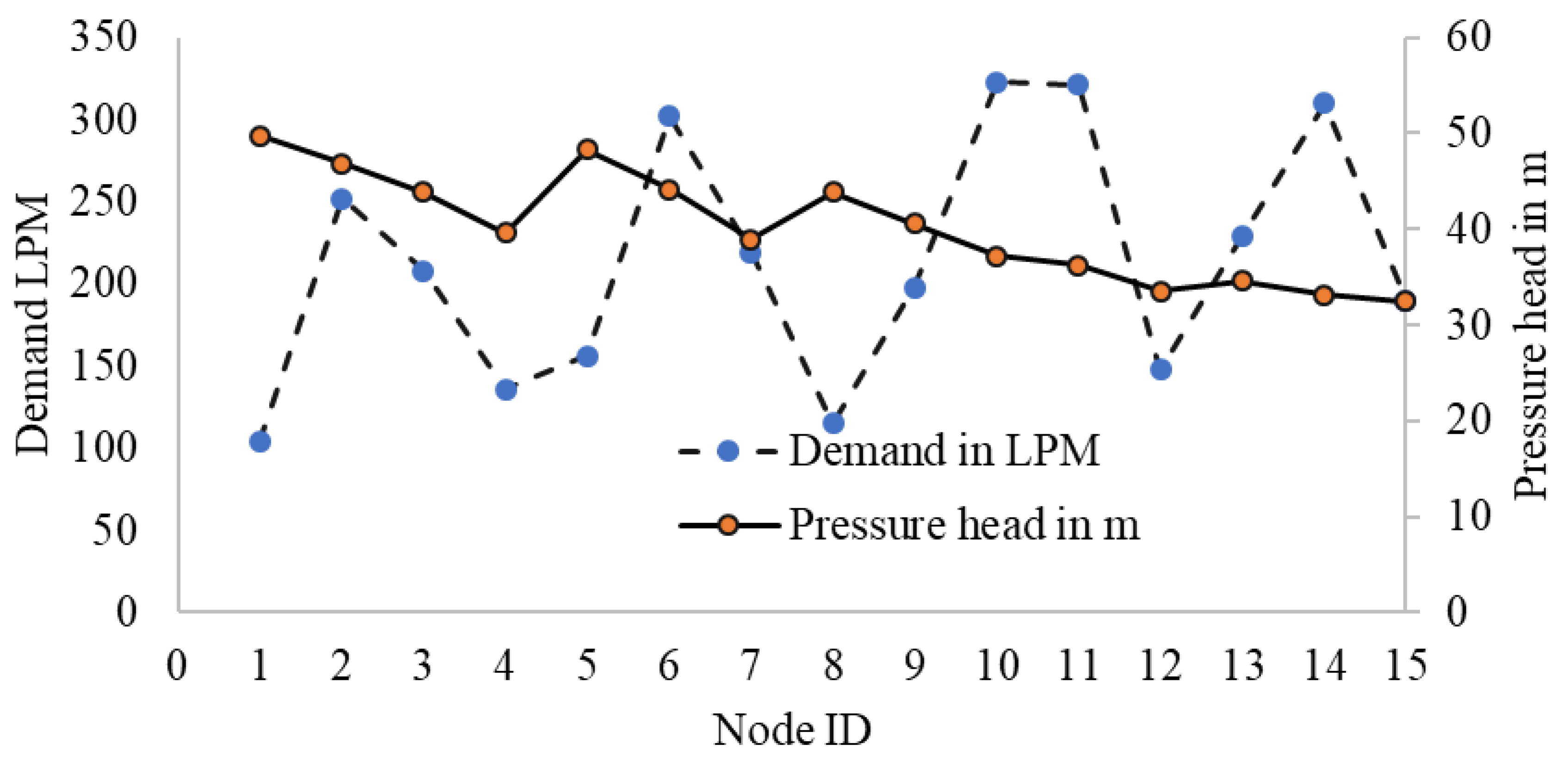
The network is simulated for peak demand, and it is found that the demand is met with the required pressure of 30 m at all nodes. According to this analysis, the network can supply all nodes when it is working under normal conditions, provided the withdrawal pattern is as per peak demand by all consumers. It can be seen from Figure 5 that when water is drawn as per peak demand/design demand, the pressure at all nodes is above 30 m, and demand will be supplied as per design value, provided that the normal condition exists. This shows that the network’s pipe configuration is appropriate to supply the demand with the required service pressure of 30 m.

The CWS system, where the house connection service is linked directly to the internal plumbing system, will supply water whenever the internal plumbing outlets are opened. The flow through the system depends on the availability of pressure. The number of plumbing outlet fixtures could vary from house to house, and all its usage simultaneously occurs very rarely. If all outlets are opened simultaneously in every house, then the flow corresponding to that situation can be considered as the peak flow of the system. However, the pipe sizing in the WDN is not decided based on such flow rate. Hence, during its functioning, the supply variations among consumers are usually noticed, and consumers are happy in some regions, satisfied in a few regions, and unsatisfied in other regions, due to the large fluctuations in pressure and supply rate. To illustrate this scenario, the emitter option available is used as a unified plumbing arrangement that can show the supply based on the pressure available at that node.

The proposed SDA approach is applied considering certain critical scenarios where every user draws water simultaneously through their available plumbing outlets. Initially, the five and two plumbing fixtures are considered in active state for all houses. Rarely could simultaneous usage of plumbing fixtures, even at peak hours, by all consumers in a street occur. Hence, the simulation is also performed with 10%, 20%, 30%, 50%, and 75% of consumers in the active conditions for two fixtures alone for illustration. 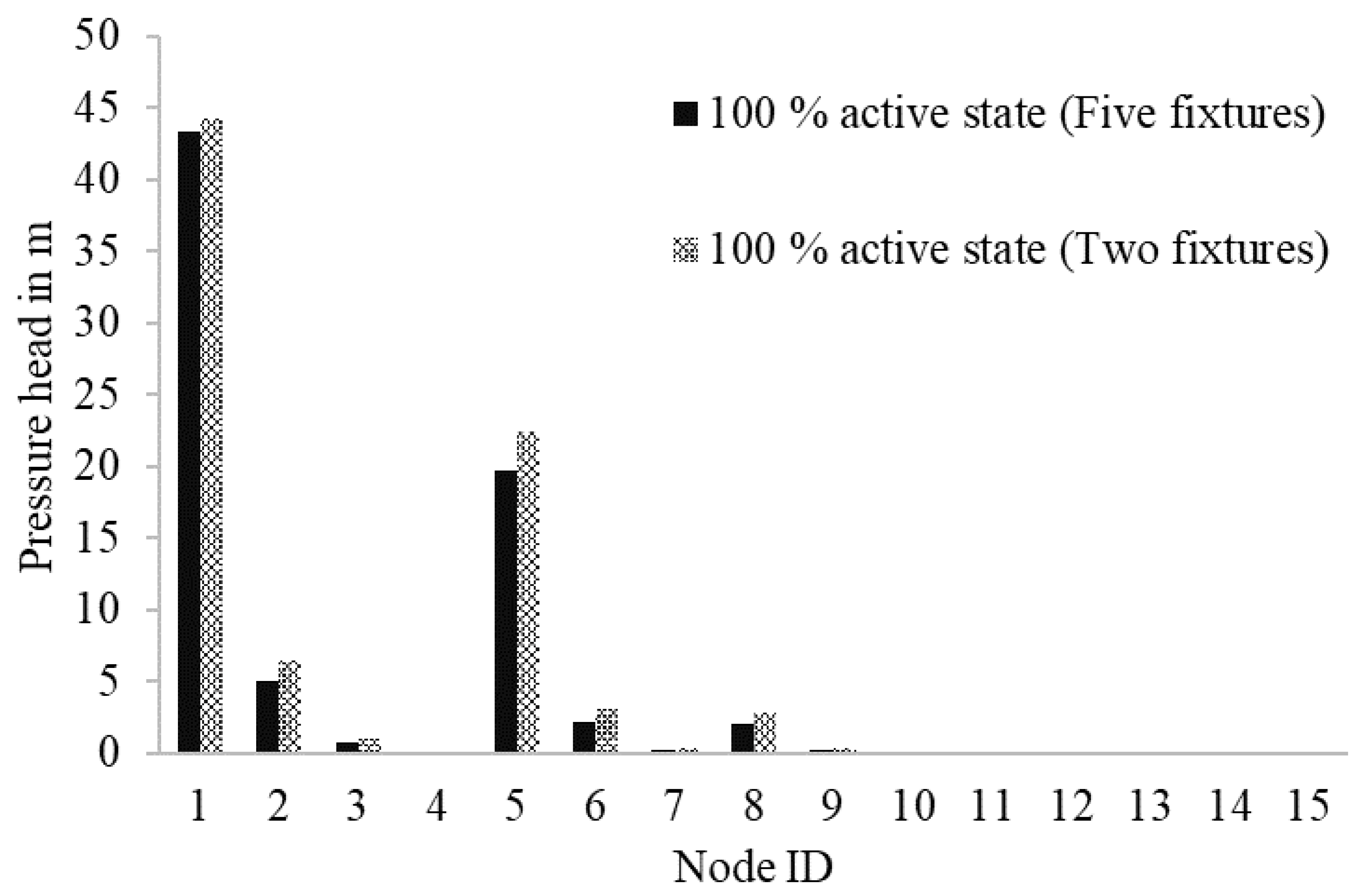To simulate using the emitter expression developed for single-, double-, and triple-story buildings, each demand node is connected with the emitter node using a 0.1 m length and 300 mm diameter pipe having a Hazen–Williams roughness coefficient of 130, as shown in Figure 3. There will be three such fictitious systems to simulate these three types of dwellings. Each fictitious pipe is supported with a fictitious check valve to prevent reverse flow. Hence, each demand node will be connected with three fictitious pipe systems. In some cases, few nodes do not have three-story buildings; then, it is enough to connect two fictitious systems. Initially, the analysis is performed with 100% active condition for two and five fixtures in operational condition. The analysis clearly shows the deprived supply to several nodes when five and two fixtures are in 100% active condition. The pressure at node 1 alone is greater than 30 m, and the remaining nodes are experiencing pressure heads less than 30 m (Figure 6). The high supply rate of water in the advantaged nodes caused a deprived supply or extremely poor supply. Further, the supply variation between two fixtures and five fixtures in the active state is minimal. It is obvious that when more fixtures are open, the flow gets distributed due to a drop in pressure despite more paths being available at that instant, and a slightly higher flow may be observed compared to the flow when two fixtures are open. These two scenarios seldom occur in reality. As the simultaneous opening of fixtures in all houses is rare, this analysis provides a theoretical observation for municipal engineers. Estimating the probability of active consumers provides a better analysis. In the absence of such data, the simulation can be carried out for a selected percentage of the consumers who are in active condition. 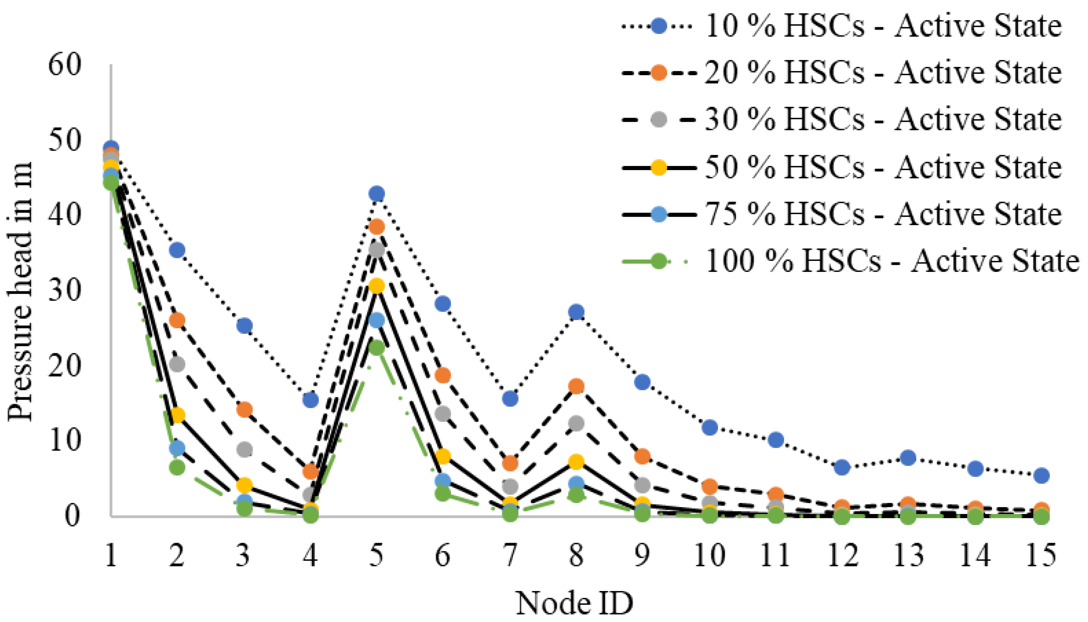Figure 7 shows the variation of nodal pressure for a different proportion of consumers in an active state. The nodal pressure falls below 30 m for 12 nodes, and still, consumers receive water when 10% of house service connections (HSC) are in the active state. This scenario changes when the level of consumers’ active state increases. The consumers living on the ground and first floors can cater to their needs. The consumers living on higher floors will be deprived of water supply due to poor pressure availability. The supply is possible only if the consumers at the advantaged nodes become inactive. The advantaged consumers always meet their requirements very quickly, and they close their fixtures as soon as the required volume is received. This could help to tide over to a certain extent for those consumers deprived at those moments.

It can be seen from Figure 8 that the consumers at nodes 1, 2, 5, and 6 receive the supply at a higher rate whenever they open their plumbing fixtures. The entire simulation is carried out with supply unit LPM. While comparing the corresponding design demand (three times the average demand) with 10% of house service connections under two fixture operating conditions, the supply-to-design demand (S/DD) ratio varies from 1.01 to 4.67 The variations observed for 20%, 30%, 50%, 5%, and 100% are (0.61 to 9.24), (0.37 to 13.75), (0.16 to 22.60), (0.07 to 33.39), and (0.04 to 43.90), respectively. The upper value of S/DD is increasing enormously while the active HSCs increase, and a reverse trend is observed for lower range values. This clearly shows, in the case of flat terrain, how consumers close to the source receive more water than those located remotely from the source. If this is visualized with respect to average demand, then the above-shown ranges shall be multiplied by three.

More realistic results can be obtained if a more accurate relationship is developed based on field measurements. As the entire simulation analysis depends on the values of the emitter coefficient and exponent, the measurement of flow from the street main to the house service line under different fixtures in active state with varying static pressure in the main pipe could help to arrive at a more accurate relationship between pressure and flow. In developed countries, water billing based on the volume of water drawn can provide the usage of water for each service connection. But it will not reflect the peak usage of water. Hence, measuring the flow and pressure at selected intervals of time in the house service connection can help the modelers accurately simulate the networks. Further, laboratory-level investigation of typical house plumbing systems under different pressure heads and operation of fixtures could help better present the flow and pressure relationship. Using such relationships in the analysis of water distribution for CWS systems can replace the current practice of demand-based design. The simulated results for 10% active consumers denote the deficit in the pressure at several nodes like other cases considered in this analysis. The pipes 1 to 5, 7, 8, 11, and 15 to 22 are revised as 400, 350, 250, 200, 300, 200, 200, 200, 200, 200, 150, 150, 150, 150, 200, and 200 mm, respectively, in order to obtain a 30 m pressure head at all supply nodes. The diameter of the pipes carrying a large quantity of flow is increased and simulated by the proposed approach. It is noticed that the pressure at all demand nodes has reached above 30 m. 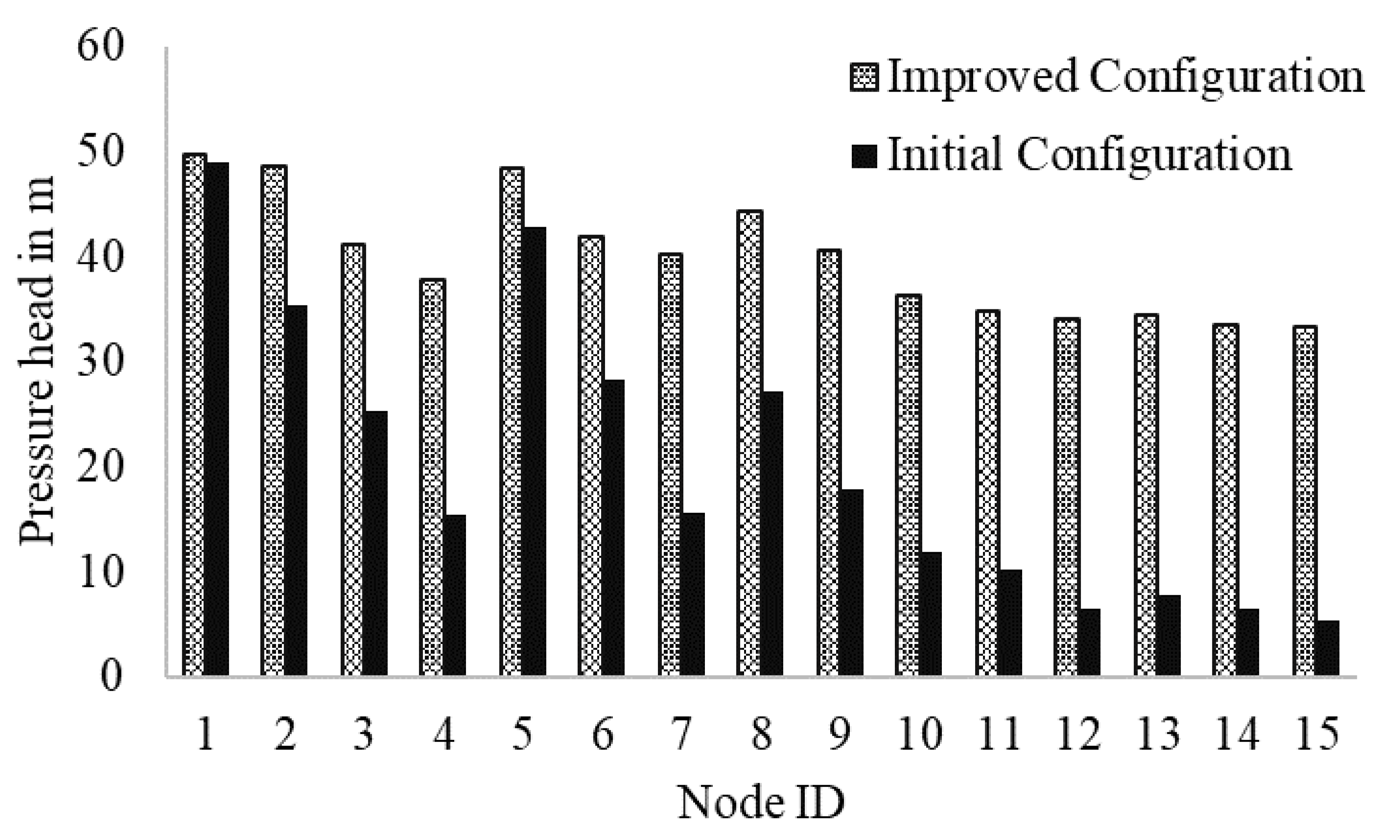Figure 9 shows the nodal pressure head for the initial and revised configurations of the network. Further, the S-DD ratio for the revised configuration has a higher value at all nodes than the initial configuration (Figure 10). The S-DD range for the revised pipe configuration (3.03–4.72) has become closer compared with the initial configuration (1.01–4.67). Further, it can be noticed from Figure 10 how the SDD ratio varies at each node for the initial and improved network configurations. The two curves become wider at the higher node numbers which are relatively far from the source. Since the pressure at all nodes is above 30 m for the revised configuration, supply to all floors is possible simultaneously when 10% HSCs are in the active condition. But, in the case of a network with the initial configuration, only partial supply at several nodes is possible. It can be understood that supply to the ground floor would be satisfied, but supply to higher floors may not be possible owing to inadequate pressure. It is evident from this study that an increase in the diameter of the pipes carrying more flow or posing more energy losses shall need to be revised suitably or optimally. In some cases, the head at the source shall be revised to maintain the service pressure. This study indicates that the peak factor (PF) varies from 9.09 to 14.15 with respect to average demand when 10% of HSCs are in the active condition for the revised configuration. The proposed analysis method can certainly be useful in the optimal design of WDNs where the sizing of pipes and fixing of the source head are the major objectives.

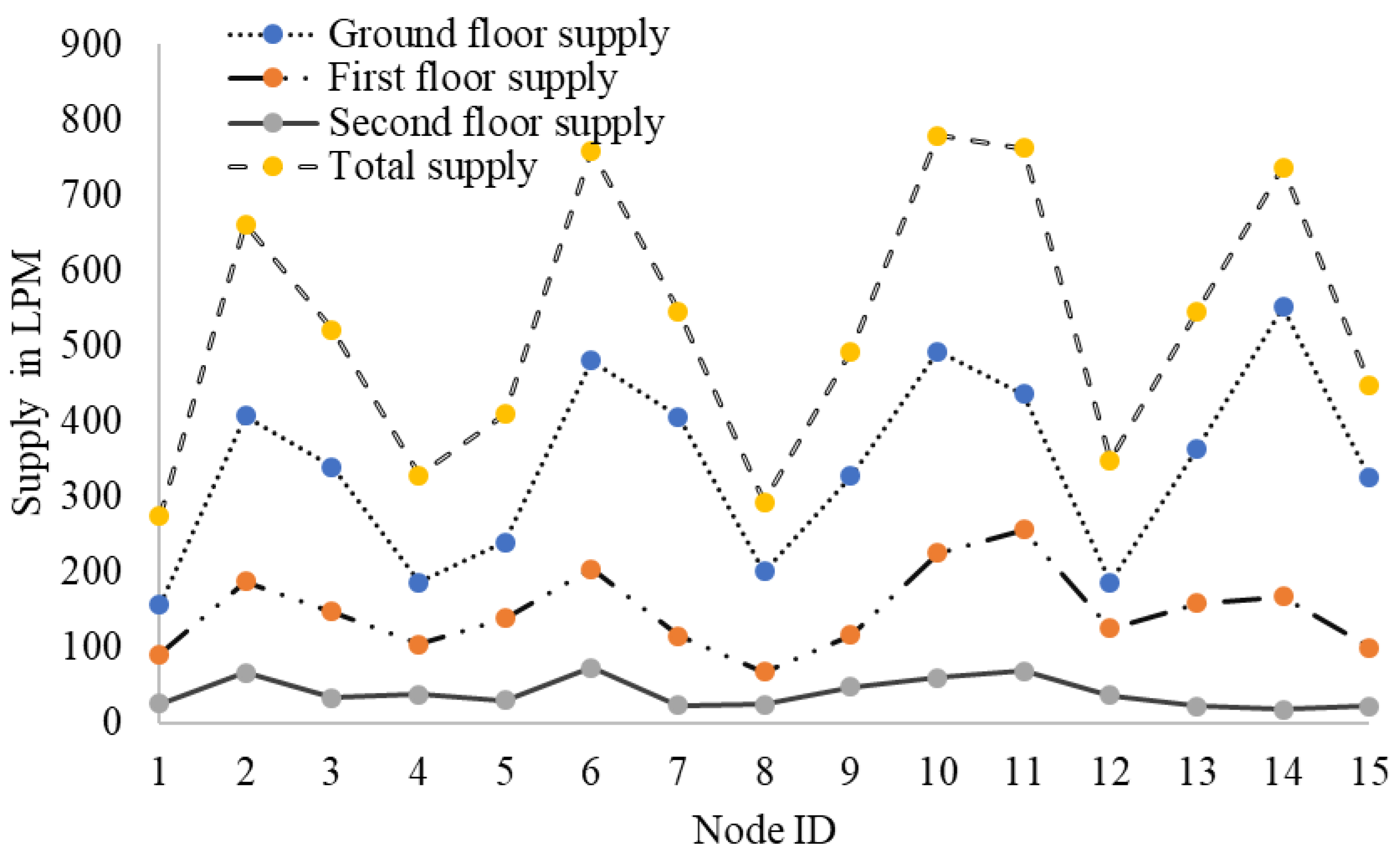
The approach described above provides the total supply for each type of building instead of the floor-wise supply rate. To know the floor-wise supply, the emitter nodes for each story shall be elevated to the level of the supply rather than following lumped supply quantification on the ground floor. To examine the effect of supply to different floors, the added fictitious emitter nodes are elevated to 1.5 m, 4.5 m, and 7.5 m, corresponding to the ground floor (GF), first floor (FF), and second floor (SF). The emitter equation corresponding to the GF is employed to simulate the supply. The simulation is performed for two fixtures in active condition for each house for different percentages of HSCs.

Table 5. Floor-wise supply when two fixtures are in operation for various percentages of HSCs in the active state.

Node ID	Floor Wise Supply Status with Two Fixtures in the Active State
	10%			20%			30%			50%			75%			100%
	GF	FF	SF	GF	FF	SF	GF	FF	SF	GF	FF	SF	GF	FF	SF	GF	FF	SF
1	Y	Y	Y	Y	Y	Y	Y	Y	Y	Y	Y	Y	Y	Y	Y	Y	Y	Y
2	Y	Y	Y	Y	Y	Y	Y	Y	Y	Y	Y	Y	Y	Y	Y	Y	Y	Y
3	Y	Y	Y	Y	Y	Y	Y	Y	Y	Y	Y	Y	Y	Y	N	Y	Y	N
4	Y	Y	Y	Y	Y	Y	Y	Y	Y	Y	Y	N	Y	N	N	Y	N	N
5	Y	Y	Y	Y	Y	Y	Y	Y	Y	Y	Y	Y	Y	Y	Y	Y	Y	Y
6	Y	Y	Y	Y	Y	Y	Y	Y	Y	Y	Y	Y	Y	Y	Y	Y	Y	Y
7	Y	Y	Y	Y	Y	Y	Y	Y	Y	Y	Y	N	Y	N	N	Y	N	N
8	Y	Y	Y	Y	Y	Y	Y	Y	Y	Y	Y	Y	Y	Y	Y	Y	Y	Y
9	Y	Y	Y	Y	Y	Y	Y	Y	Y	Y	Y	N	Y	N	N	Y	N	N
10	Y	Y	Y	Y	Y	Y	Y	Y	N	Y	N	N	Y	N	N	Y	N	N
11	Y	Y	Y	Y	Y	Y	Y	Y	N	Y	N	N	Y	N	N	Y	N	N
12	Y	Y	Y	Y	Y	N	Y	N	N	Y	N	N	Y	N	N	Y	N	N
13	Y	Y	Y	Y	Y	N	Y	Y	N	Y	N	N	Y	N	N	Y	N	N
14	Y	Y	Y	Y	Y	N	Y	N	N	Y	N	N	Y	N	N	Y	N	N
15	Y	Y	Y	Y	Y	N	Y	N	N	Y	N	N	Y	N	N	Y	N	N

Y—Supply reaching; N—Supply not reaching.

presents the floor-wise supply at each node. It can be seen from Table 5 that supply is possible to all floors when 10% of HSCs are in the active state. From 20% onwards, supply to certain floors does not occur due to inadequate pressure. In the case when 100% of HSCs are in the active state, the supply is only possible on the GF at all nodes, and no supply occurs on the first and second floors for most of the nodes except those nodes located near the source. Figure 11 shows the nodal supply for the initial and improved configurations. The nodal pressure at all the nodes is found to be greater than 30 m in the case of the improved network configuration, whereas in the initial configuration, the pressure varies from 15 m to 47 m. Though the initial configuration ensures supply to all floors when 10% of HSCs are in the active state, it is unable to supply water with the required pressure of 30 m. The total rate of supply for the initial and improved configurations is obtained as 5551.39 LPM and 7914.47 LPM, respectively, when 10% of HSCs are in the active state. The pipe size of the main pipe plays a vital role in maintaining pressure. Hence, the current practice of pipe selection, either by thumb rule or optimization, will not provide a practically feasible solution. Certainly, this study will draw a design practice followed for pipe sizing based on nodal demand.

Table 6. Supply rate (LPM) per connection when 10% HSCs are in the active state.

Configuration	Ground Floor		First Floor		Second Floor
	Maximum	Minimum	Maximum	Minimum	Maximum	Minimum
Initial configuration network	406.75	101.82	170.73	46.68	60.12	7.8
Upgraded configuration network	552.05	157.28	256.94	67.66	73.38	18.16

gives the rate of supply per connection for the initial and upgraded network configurations. There is a large difference between the minimum and maximum supply to all floor levels in the case of the initial configuration. This difference appears to be smaller for the upgraded configuration. It is evident from this study that the rate of supply increases when the availability of pressure is higher. Further, it is to be noted that the flow rate per connection decreases when the floor levels increase. Figure 11 and Figure 12 provide the rate of supply at each node for the initial and upgraded configurations when 10% of HSCs are in the active state. The supply of water to each floor varies for both configurations. The variation appears large in the initial configuration. It is clear from this study that the rate of supply depends on pressure availability, and proper water main and sub-main pipe sizing is important to provide a reliable supply of water to consumers. The proposed approach can be used to assess the performance of different design alternatives, such as the pipe diameter, number of connections, active number of fixtures, placement of valves, and source head. The use of the proposed approach for the design of continuous water supply system networks can help engineers and planners to optimize network performance, reduce costs, and ensure the reliable delivery of safe and clean water to users. The limitations of the proposed analysis are that (i) the analysis adopts a steady state condition, and (ii) the transient flow that occurs in the system due to the closure of various valves is not accounted. This method can be adopted in all topologies of dwellings.

5. Conclusions

This paper presents the modeling method for the quantification of a pressure-based supply of water from the water main pipe to the house service pipe due to the opening of the fixtures at the house level. A new supply-driven concept is introduced for the analysis of WDN, where nodal demand is defined for the network in terms of the number of HSCs instead of traditional peak nodal demand. As the usual nodal peak demand estimated by multiplying the peak factor does not reflect the true peak demand, employing the proposed approach in the design of new WDNs can result in a better design and the identification of the nodes that could experience pressure deficit in the existing systems. The pressure and supply relationship obtained between the water main and HSCs can easily be adopted in the emitter tool available in the hydraulic simulation software (EPANET 2.2). The analysis using the proposed method indicates that the simultaneous opening of several plumbing fixtures could result in a major pressure deficit in the network, whereas the same network indicates that nodal demand is met with the required pressure when it is analyzed for peak demand. While analyzing with 10% active consumers in the system, close matching is found with peak demand-based analysis. This reinforces the need that certain pipes be increased its size, or the source head be increased owing to the peak supply that occurs when simultaneously opening the plumbing fixtures in the houses. The design of a water distribution network based on the projected population in the area helps to size the capacity of the storage system, whereas the projected number of house service connections and potential delivery of water when the fixtures are in the active state will be useful for the sizing of the pipes and pumps. The analysis depicts that the supply of large volumes of water at the high-pressure nodes in a relatively short time leads to a very high PF for which the main piping system is not designed. High friction loss in the main pipes that carry flow to nodes distant from the source creates pressure-deficient conditions. This study has also shown how an increase in the size of the pipe configuration of the network results in improved performance in terms of supply with required service pressure. The analysis additionally emphasizes the use of elevated fictitious nodes for each floor in evaluating the supply rate in the modeling. This paper further recommends additional theoretical and field research related to the pressure and supply of water at the various story buildings with respect to time that could help improve the pipe sizing design of water distribution networks.