Time Series Clustering: A Complex Network-Based Approach for Feature Selection in Multi-Sensor Data


Abstract
:1. Introduction
2. Background
2.1. Feature Subset Selection
2.1.1. Time Series Clustering
2.1.2. Evaluation Metrics for Unsupervised FSS
2.2. Complex Network Analysis
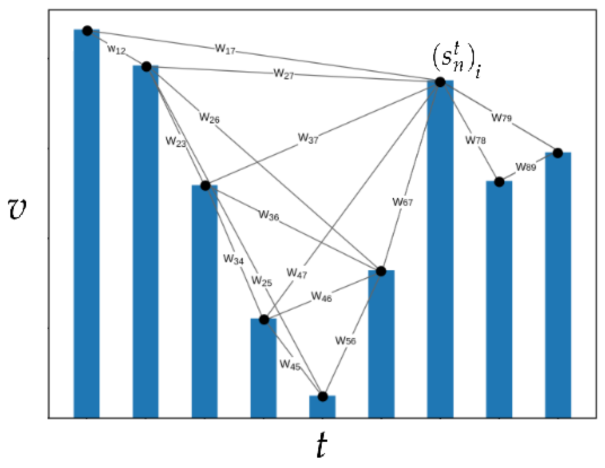
2.2.1. Visibility Graph
2.2.2. Local Network Measures
2.2.3. Community Detection
Visualization
Evaluation Metrics
3. Methods
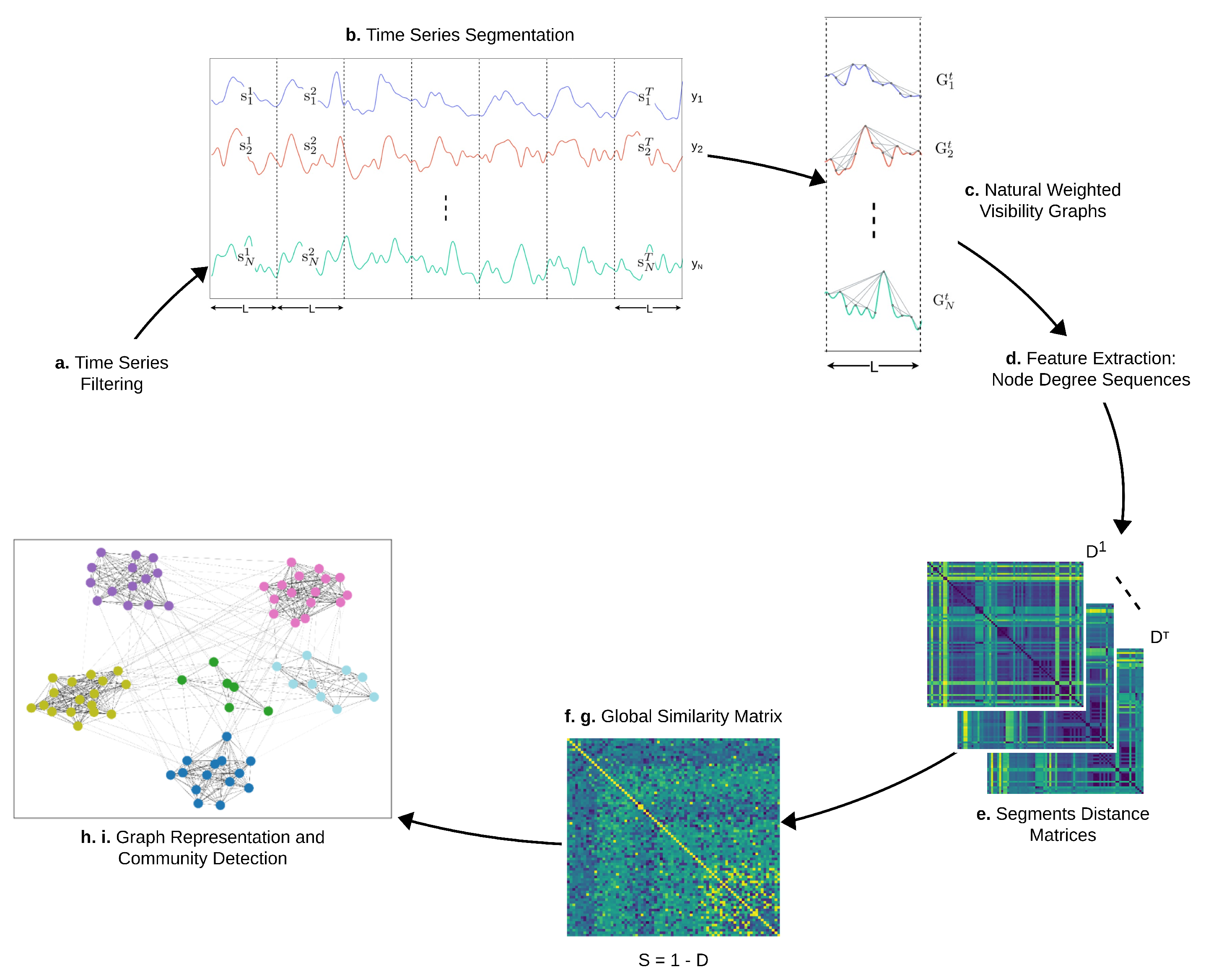
- Remove time series noise through a low-pass filter.
- Segment time series into consecutive non-overlapping intervals corresponding to a fixed time amplitude L, where T is the number of segments extracted for each time series.
- Transform every signal segment ( and ) into a weighted natural visibility graph .
- Construct a feature vector for each visibility graph , where is the degree centrality of the ith node in the graph and the degree sequence of the graph.
- Define a distance matrix for every tth segment (, where the entry is the Euclidean distance between the degree centrality vectors and . Every matrix gives a measure of how different every pair of time series is in the tth segment.
- Compute a global distance matrix D that covers the full time period T where the entry is computed as , averaging the contributions of the individual distance matrices associated to every segment.
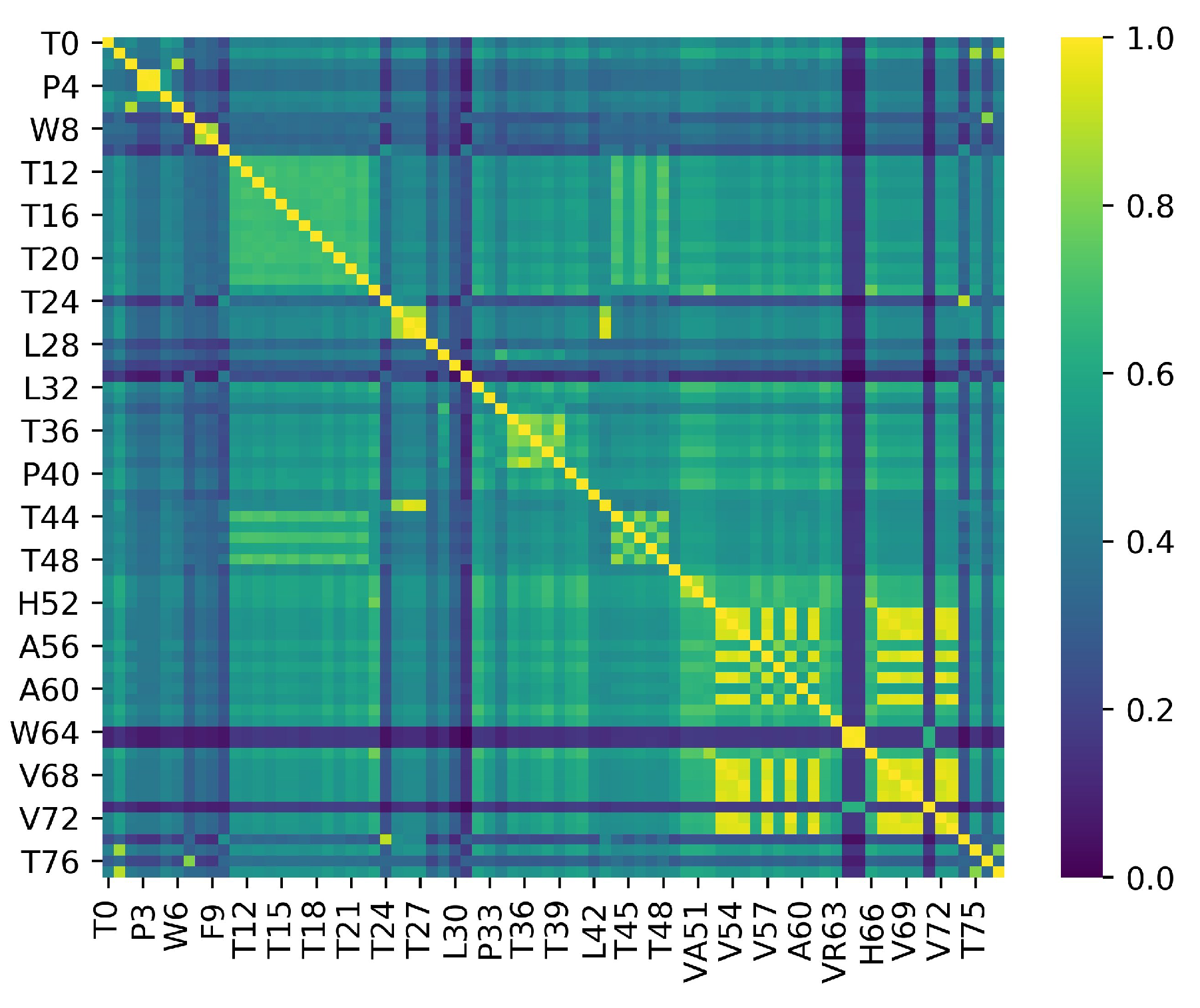
- Normalize D between 0 and 1, making it possible to define a similarity matrix as , which measures how similar every pair of time series is over the full time period.
- Build a weighted graph C considering S as an adjacency matrix.
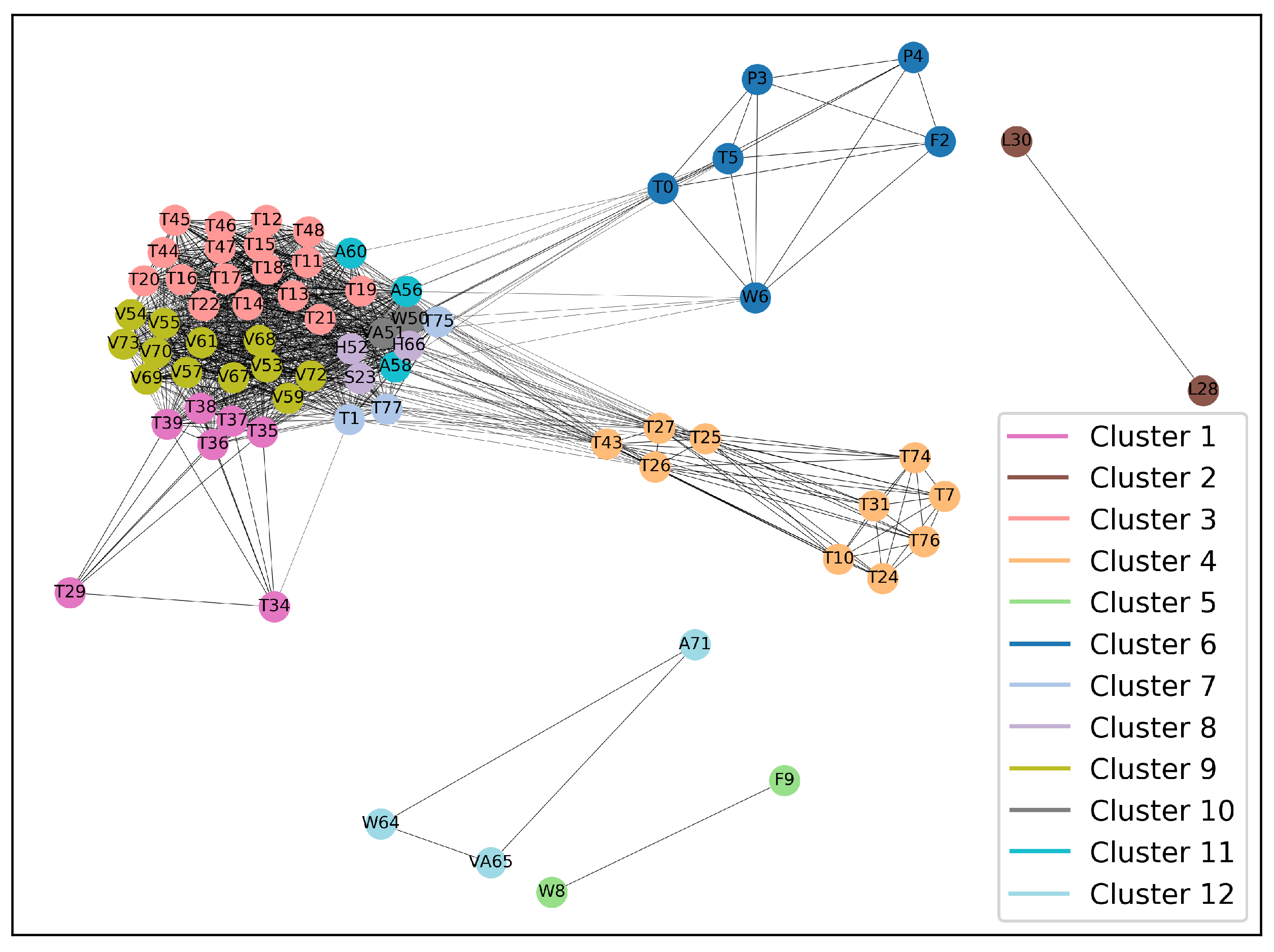
- Cluster the original time series by applying a community detection algorithm on the graph C and visualize the results through a force-directed layout.
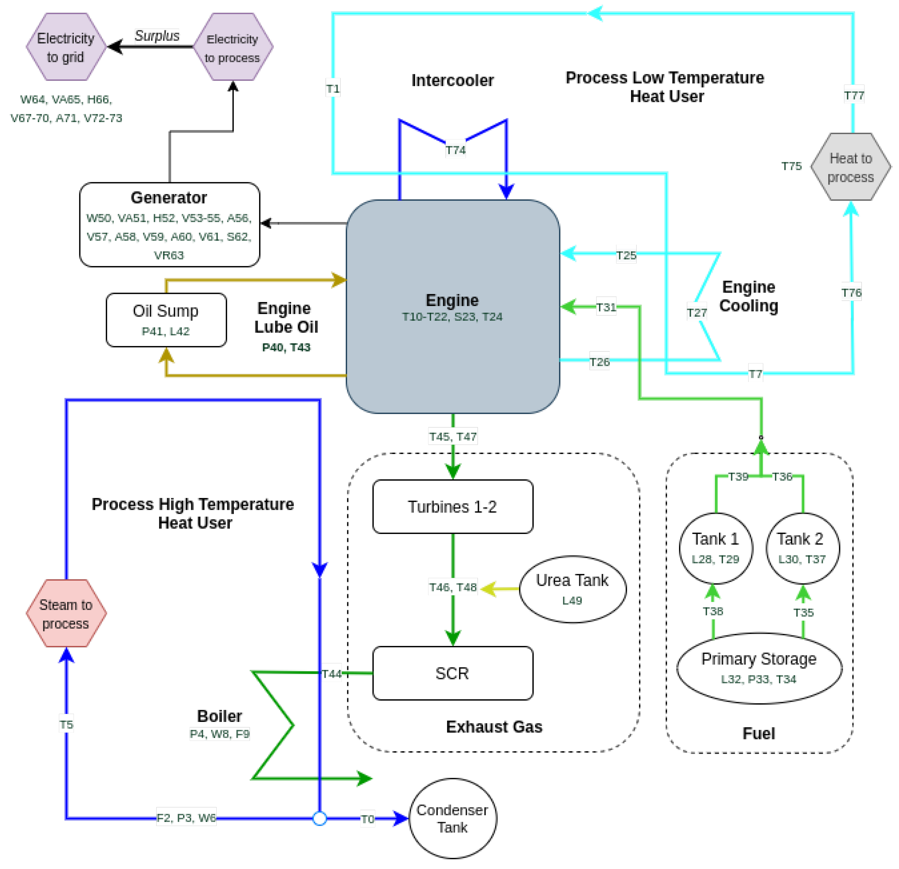
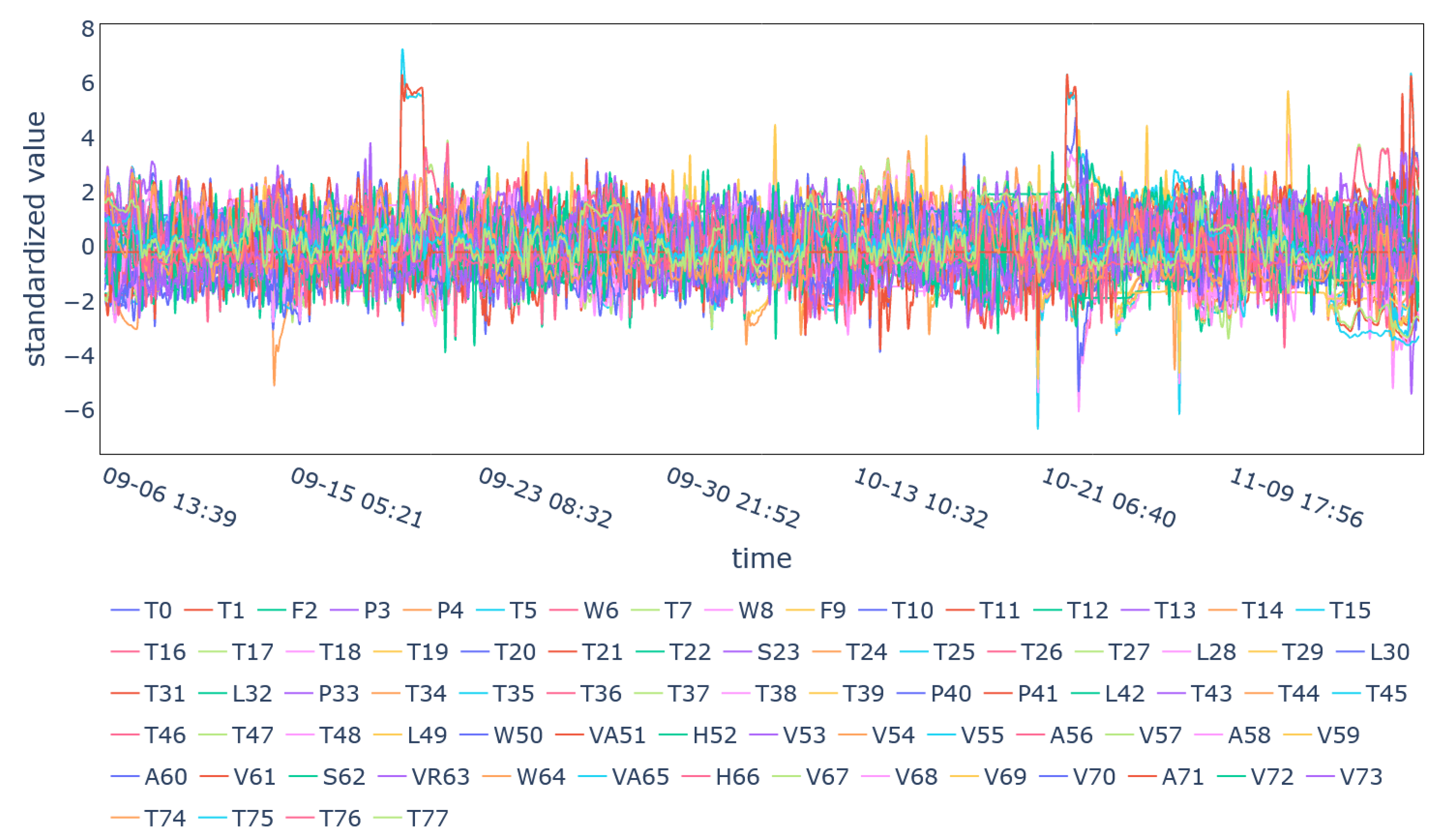
4. Case Study
5. Results
Performance Metrics
6. Conclusions
Author Contributions
Funding
Conflicts of Interest
References
- Mohammadi, M.; Al-Fuqaha, A.; Sorour, S.; Guizani, M. Deep Learning for IoT Big Data and Streaming Analytics: A Survey. IEEE Commun. Surv. Tutor. 2018, 20, 2923–2960. [Google Scholar] [CrossRef] [Green Version]
- Asghari, P.; Rahmani, A.M.; Javadi, H.H. Internet of Things applications: A systematic review. Comput. Netw. 2019, 148, 241–261. [Google Scholar] [CrossRef]
- Imkamp, D.; Berthold, J.; Heizmann, M.; Kniel, K.; Manske, E.; Peterek, M.; Schmitt, R.; Seidler, J.; Sommer, K.D. Challenges and trends in manufacturing measurement technology—The “Industrie 4.0” concept. J. Sensors Sensor Syst. 2016, 5, 325. [Google Scholar] [CrossRef] [Green Version]
- Lu, Y. Industry 4.0: A survey on technologies, applications and open research issues. J. Ind. Inf. Integr. 2017, 6, 1–10. [Google Scholar]
- Hayes-Roth, B.; Washington, R.; Hewett, R.; Hewett, M.; Seiver, A. Intelligent Monitoring and Control. In Proceedings of the IJCAI, Detroit, MI, USA, 20–25 August 1989; Volume 89, pp. 243–249. [Google Scholar]
- Verleysen, M.; François, D. The curse of dimensionality in data mining and time series prediction. In International Work-Conference on Artificial Neural Networks; Springer: New York, NY, USA, 2005; pp. 758–770. [Google Scholar]
- Uraikul, V.; Chan, C.W.; Tontiwachwuthikul, P. Artificial intelligence for monitoring and supervisory control of process systems. Eng. Appl. Artif. Intell. 2007, 20, 115–131. [Google Scholar]
- Tian, H.X.; Liu, X.J.; Han, M. An outliers detection method of time series data for soft sensor modeling. In Proceedings of the 2016 Chinese Control and Decision Conference (CCDC), Yinchuan, China, 28–30 May 2016; pp. 3918–3922. [Google Scholar]
- Kaiser, J. Dealing with missing values in data. J. Syst. Integr. 2014, 5, 42–51. [Google Scholar] [CrossRef]
- Liu, R.; Yang, B.; Zio, E.; Chen, X. Artificial intelligence for fault diagnosis of rotating machinery: A review. Mech. Syst. Signal Process. 2018, 108, 33–47. [Google Scholar] [CrossRef]
- Ruiz-Sarmiento, J.R.; Monroy, J.; Moreno, F.A.; Galindo, C.; Bonelo, J.M.; Gonzalez-Jimenez, J. A predictive model for the maintenance of industrial machinery in the context of Industry 4.0. Eng. Appl. Artif. Intell. 2020, 87, 103289. [Google Scholar] [CrossRef]
- Ansari, F.; Glawar, R.; Nemeth, T. PriMa: A prescriptive maintenance model for cyber-physical production systems. Int. J. Comput. Integr. Manuf. 2019, 32, 482–503. [Google Scholar]
- Jin, X.; Shao, J.; Zhang, X.; An, W.; Malekian, R. Modeling of nonlinear system based on deep learning framework. Nonlinear Dyn. 2016, 84, 1327–1340. [Google Scholar] [CrossRef] [Green Version]
- Chormunge, S.; Jena, S. Correlation based feature selection with clustering for high dimensional data. J. Electr. Syst. Inf. Technol. 2018, 5, 542–549. [Google Scholar] [CrossRef]
- Frolik, J.; Abdelrahman, M. Synthesis of quasi-redundant sensor data: A probabilistic approach. In Proceedings of the 2000 American Control Conference. ACC (IEEE Cat. No. 00CH36334), Chicago, IL, USA, 28–30 June 2000; Volume 4, pp. 2917–2921. [Google Scholar]
- Acid, S.; De Campos, L.M.; Fernández, M. Minimum redundancy maximum relevancy versus score-based methods for learning Markov boundaries. In Proceedings of the 2011 11th International Conference on Intelligent Systems Design and Applications, Cordoba, Spain, 22–24 November 2011; pp. 619–623. [Google Scholar]
- Chandrashekar, G.; Sahin, F. A survey on feature selection methods. Comput. Electr. Eng. 2014, 40, 16–28. [Google Scholar] [CrossRef]
- You, D.; Wu, X.; Shen, L.; He, Y.; Yuan, X.; Chen, Z.; Deng, S.; Ma, C. Online Streaming Feature Selection via Conditional Independence. Appl. Sci. 2018, 8, 2548. [Google Scholar] [CrossRef] [Green Version]
- Pal, S.K.; Mitra, P. Pattern Recognition Algorithms for Data Mining: Scalability, Knowledge Discovery, and Soft Granular Computing; Chapman & Hall, Ltd.: London, UK, 2004. [Google Scholar]
- Song, Q.; Ni, J.; Wang, G. A fast clustering-based feature subset selection algorithm for high-dimensional data. IEEE Trans. Knowl. Data Eng. 2011, 25, 1–14. [Google Scholar] [CrossRef]
- Baker, L.D.; McCallum, A.K. Distributional clustering of words for text classification. In Proceedings of the 21st Annual International ACM SIGIR Conference on Research and Development in Information Retrieval, Melbourne, Australia, 24–28 August 1998; pp. 96–103. [Google Scholar]
- Slonim, N.; Tishby, N. The power of word clusters for text classification. In Proceedings of the 23rd European Colloquium on Information Retrieval Research, Darmstadt, Germany, 4–6 April 2001; Volume 1, p. 200. [Google Scholar]
- Zou, Y.; Donner, R.; Marwan, N.; Donges, J.; Kurths, J. Complex network approaches to nonlinear time series analysis. Phys. Rep. 2018, 787, 1–97. [Google Scholar] [CrossRef]
- Lacasa, L.; Luque, B.; Ballesteros, F.; Luque, J.; Nuño, J.C. From time series to complex networks: The visibility graph. Proc. Natl. Acad. Sci. USA 2008, 105, 4972–4975. [Google Scholar]
- Koschützki, D.; Schreiber, F. Centrality analysis methods for biological networks and their application to gene regulatory networks. Gene Regul. Syst. Biol. 2008, 2, GRSB–S702. [Google Scholar]
- Blondel, V.D.; Guillaume, J.L.; Lambiotte, R.; Lefebvre, E. Fast unfolding of communities in large networks. J. Stat. Mech. Theory Exp. 2008, 2008, P10008. [Google Scholar] [CrossRef] [Green Version]
- Lal, T.N.; Chapelle, O.; Weston, J.; Elisseeff, A. Embedded methods. In Feature Extraction; Springer: New York, NY, USA, 2006; pp. 137–165. [Google Scholar]
- Kohavi, R.; John, G.H. Wrappers for feature subset selection. Artif. Intell. 1997, 97, 273–324. [Google Scholar] [CrossRef] [Green Version]
- Sánchez-Maro no, N.; Alonso-Betanzos, A.; Tombilla-Sanromán, M. Filter methods for feature selection—A comparative study. In Proceedings of the International Conference on Intelligent Data Engineering and Automated Learning, Birmingham, UK, 16–19 December 2007; pp. 178–187. [Google Scholar]
- Brahim, A.B.; Limam, M. A hybrid feature selection method based on instance learning and cooperative subset search. Pattern Recognit. Lett. 2016, 69, 28–34. [Google Scholar]
- Hauskrecht, M.; Pelikan, R.; Valko, M.; Lyons-Weiler, J. Feature selection and dimensionality reduction in genomics and proteomics. In Fundamentals of Data Mining in Genomics and Proteomics; Springer: New York, NY, USA, 2007; pp. 149–172. [Google Scholar]
- Sanche, R.; Lonergan, K. Variable reduction for predictive modeling with clustering. In Casualty Actuarial Society Forum; Casualty Actuarial Society: Arlington, VA, USA, 2006; pp. 89–100. [Google Scholar]
- Fritzke, B. Unsupervised clustering with growing cell structures. In Proceedings of the IJCNN-91-Seattle International Joint Conference on Neural Networks, Seattle, WA, USA, 8–12 July 1991; Volume 2, pp. 531–536. [Google Scholar]
- Clarkson, B.; Pentland, A. Unsupervised clustering of ambulatory audio and video. In Proceedings of the 1999 IEEE International Conference on Acoustics, Speech, and Signal Processing, Phoenix, AZ, USA, 15–19 March 1999; Volume 6, pp. 3037–3040. [Google Scholar]
- Popat, S.K.; Emmanuel, M. Review and comparative study of clustering techniques. Int. J. Comput. Sci. Inf. Technol. 2014, 5, 805–812. [Google Scholar]
- Fujita, A.; Sato, J.; Demasi, M.; Sogayar, M.; Ferreira, C.; Miyano, S. Comparing Pearson, Spearman and Hoeffding’s D measure for gene expression association analysis. J. Bioinf. Comput. Biol. 2009, 7, 663–684. [Google Scholar] [CrossRef] [PubMed]
- Iglesias, F.; Kastner, W. Analysis of Similarity Measures in Times Series Clustering for the Discovery of Building Energy Patterns. Energies 2013, 6, 579–597. [Google Scholar] [CrossRef] [Green Version]
- Jing, L.; Ng, M.; Huang, J. An Entropy Weighting K-Means Algorithm for Subspace Clustering of High-Dimensional Sparse Data. IEEE Trans. Knowl. Data Eng. 2007, 19, 1026–1041. [Google Scholar] [CrossRef]
- Huang, X.; Ye, Y.; Zhang, H. Extensions of Kmeans-Type Algorithms: A New Clustering Framework by Integrating Intracluster Compactness and Intercluster Separation. IEEE Trans. Neural Netw. Learn. Syst. 2014, 25, 1433–1446. [Google Scholar] [CrossRef] [PubMed]
- Baragona, R. A simulation study on clustering time series with metaheuristic methods. Quad. Stat. 2001, 3, 1–26. [Google Scholar]
- Ramoni, M.; Sebastiani, P.; Cohen, P.R. Multivariate Clustering by Dynamics. In Proceedings of the Seventeenth National Conference on Artificial Intelligence and Twelfth Conference on Innovative Applications of Artificial Intelligence, Austin, TX, USA, 30 July–3 August 2000; pp. 633–638. [Google Scholar]
- Tran, D.; Wagner, M. Fuzzy c-means clustering-based speaker verification. In Proceedings of the AFSS International Conference on Fuzzy Systems; Springer: New York, NY, USA, 2002; pp. 318–324. [Google Scholar]
- Bandara, K.; Bergmeir, C.; Smyl, S. Forecasting across time series databases using recurrent neural networks on groups of similar series: A clustering approach. Exp. Syst. Appl. 2020, 140, 112896. [Google Scholar] [CrossRef] [Green Version]
- Shaw, C.; King, G. Using cluster analysis to classify time series. Phys. D Nonlinear Phenom. 1992, 58, 288–298. [Google Scholar] [CrossRef]
- Vlachos, M.; Lin, J.; Keogh, E.; Gunopulos, D. A Wavelet-Based Anytime Algorithm for K-Means Clustering of Time Series. In Proceedings of the Workshop on Clustering High Dimensionality Data and Its Applications, San Francisco, CA, USA, 3 May 2003; pp. 23–30. [Google Scholar]
- Kavitha, V.; Punithavalli, M. Clustering Time Series Data Stream—A Literature Survey. arXiv 2010, arXiv:1005.4270. [Google Scholar]
- Rani, S.; Sikka, G. Recent Techniques of Clustering of Time Series Data: A Survey. Int. J. Comput. Appl. 2012, 52, 1–9. [Google Scholar] [CrossRef]
- Aghabozorgi, S.; Shirkhorshidi, A.S.; Wah, T. Time-series clustering—A decade review. Inf. Syst. 2015, 53, 16–38. [Google Scholar] [CrossRef]
- Zanin, M.; Papo, D.; Sousa, P.A.; Menasalvas, E.; Nicchi, A.; Kubik, E.; Boccaletti, S. Combining complex networks and data mining: Why and how. Phys. Rep. 2016, 635, 1–44. [Google Scholar] [CrossRef] [Green Version]
- Ferreira, L.; Zhao, L. Time Series Clustering via Community Detection in Networks. Inf. Sci. 2015, 326. [Google Scholar] [CrossRef] [Green Version]
- Zhang, X.; Liu, J.; Du, Y.; Lu, T. A novel clustering method on time series data. Exp. Syst. Appl. 2011, 38, 11891–11900. [Google Scholar] [CrossRef]
- Shannon, C.E. A mathematical theory of communication. Bell Syst. Tech. J. 1948, 27, 379–423. [Google Scholar] [CrossRef] [Green Version]
- Lozano-Pérez, T.; Wesley, M.A. An Algorithm for Planning Collision-Free Paths among Polyhedral Obstacles. Commun. ACM 1979, 22, 560–570. [Google Scholar] [CrossRef]
- Luque, B.; Lacasa, L.; Ballesteros, F.; Luque, J. Horizontal visibility graphs: Exact results for random time series. Phys. Rev. E 2009, 80, 046103. [Google Scholar] [CrossRef] [Green Version]
- Lacasa, L.; Toral, R. Description of stochastic and chaotic series using visibility graphs. Phys. Rev. E 2010, 82, 036120. [Google Scholar] [CrossRef] [Green Version]
- Bianchi, F.M.; Livi, L.; Alippi, C.; Jenssen, R. Multiplex visibility graphs to investigate recurrent neural network dynamics. Sci. Rep. 2017, 7, 1–13. [Google Scholar] [CrossRef] [Green Version]
- Bonacich, P. Some unique properties of eigenvector centrality. Soc. Netw. 2007, 29, 555–564. [Google Scholar] [CrossRef]
- Freeman, L.C. Centrality in social networks conceptual clarification. Soc. Netw. 1978, 1, 215–239. [Google Scholar]
- Scott, J. Social Network Analysis. Sociology 1988, 22, 109–127. [Google Scholar] [CrossRef]
- Freeman, L. The development of social network analysis. Study Sociol. Sci. 2004, 1, 687. [Google Scholar]
- Rice, S.A. The identification of blocs in small political bodies. Am. Pol. Sci. Rev. 1927, 21, 619–627. [Google Scholar] [CrossRef]
- Weiss, R.S.; Jacobson, E. A method for the analysis of the structure of complex organizations. Am. Sociol. Rev. 1955, 20, 661–668. [Google Scholar] [CrossRef]
- Homans, G.C. The Human Group; Routledge: London, UK, 2013. [Google Scholar]
- Fortunato, S. Community detection in graphs. Phys. Rep. 2010, 486, 75–174. [Google Scholar]
- Kernighan, B.W.; Lin, S. An Efficient Heuristic Procedure for Partitioning Graphs. Bell Syst. Tech. J. 1970, 49, 291–307. [Google Scholar] [CrossRef]
- Barnes, E. An algorithm for partitioning the nodes of a graph. In Proceedings of the 1981 20th IEEE Conference on Decision and Control including the Symposium on Adaptive Processes, San Diego, CA, USA, 16–18 December 1981; pp. 303–304. [Google Scholar]
- Lloyd, S.P. Least Squares Quantization in PCM. IEEE Trans. Inf. Theory 1982, 28, 129–137. [Google Scholar] [CrossRef]
- Friedman, J.; Hastie, T.; Tibshirani, R. The Elements of Statistical Learning; Springer: New York, NY, USA, 2001; Volume 1. [Google Scholar]
- Newman, M.E. Fast algorithm for detecting community structure in networks. Phys. Rev. E 2004, 69, 066133. [Google Scholar] [CrossRef] [Green Version]
- Guimera, R.; Sales-Pardo, M.; Amaral, L.A.N. Modularity from fluctuations in random graphs and complex networks. Phys. Rev. E 2004, 70, 025101. [Google Scholar]
- Duch, J.; Arenas, A. Community detection in complex networks using extremal optimization. Phys. Rev. E 2005, 72, 027104. [Google Scholar] [CrossRef] [PubMed] [Green Version]
- Newman, M.E.; Girvan, M. Finding and evaluating community structure in networks. Phys. Rev. E 2004, 69, 026113. [Google Scholar]
- Donath, W.E.; Hoffman, A.J. Lower bounds for the partitioning of graphs. In Selected Papers Of Alan J Hoffman: With Commentary; World Scientific: Singapore, 2003; pp. 437–442. [Google Scholar]
- Hastings, M.B. Community detection as an inference problem. Phys. Rev. E 2006, 74, 035102. [Google Scholar]
- Newman, M.E.; Leicht, E.A. Mixture models and exploratory analysis in networks. Proc. Natl. Acad. Sci. USA 2007, 104, 9564–9569. [Google Scholar] [CrossRef] [PubMed] [Green Version]
- Shannon, P.T.; Grimes, M.; Kutlu, B.; Bot, J.J.; Galas, D.J. RCytoscape: Tools for exploratory network analysis. BMC Bioinf. 2013, 14, 217. [Google Scholar] [CrossRef] [PubMed] [Green Version]
- Sakkalis, V. Review of advanced techniques for the estimation of brain connectivity measured with EEG/MEG. Comput. Biol. Med. 2011, 41, 1110–1117. [Google Scholar] [CrossRef]
- Fruchterman, T.M.; Reingold, E.M. Graph drawing by force-directed placement. Softw. Pract. Exp. 1991, 21, 1129–1164. [Google Scholar] [CrossRef]
- Liu, X.; Cheng, H.M.; Zhang, Z.Y. Evaluation of community detection methods. IEEE Trans. Knowl. Data Eng. 2019, in press. [Google Scholar]
- Manning, C.D.; Raghavan, P.; Schütze, H. Introduction to Information Retrieval; Cambridge University Press: Cambridge, UK, 2008. [Google Scholar]
- Rand, W.M. Objective criteria for the evaluation of clustering methods. J. Am. Stat. Assoc. 1971, 66, 846–850. [Google Scholar]
- Danon, L.; Diaz-Guilera, A.; Duch, J.; Arenas, A. Comparing community structure identification. J. Stat. Mech. Theory Exp. 2005, 2005, P09008. [Google Scholar] [CrossRef]
- Ahn, Y.Y.; Bagrow, J.P.; Lehmann, S. Link communities reveal multiscale complexity in networks. Nature 2010, 466, 761–764. [Google Scholar] [CrossRef] [Green Version]
- Luque, B.; Lacasa, L. Canonical Horizontal Visibility Graphs are uniquely determined by their degree sequence. Eur. Phys. J. Spec. Top. 2016, 226. [Google Scholar] [CrossRef] [Green Version]
- Corsini, A.; Bonacina, F.; Feudo, S.; Marchegiani, A.; Venturini, P. Internal Combustion Engine sensor network analysis using graph modeling. Energy Procedia 2017, 126, 907–914. [Google Scholar] [CrossRef]
- Van Rossum, G.; Drake, F.L., Jr. Python Reference Manual; Centrum voor Wiskunde en Informatica Amsterdam: Amsterdam, The Netherlands, 1995. [Google Scholar]
- Oliphant, T.E. A Guide to NumPy; Trelgol Publishing USA: Spanish Fork, UT, USA, 2006; Volume 1. [Google Scholar]
- Hagberg, A.; Swart, P.; Chult, D. Exploring Network Structure, Dynamics, and Function Using NetworkX. In Proceedings of the 7th Python in Science Conference, Pasadena, CA, USA, 19–24 August 2008; pp. 11–15. [Google Scholar]


| ID | Variable | ID | Variable | ID | Variable |
|---|---|---|---|---|---|
| T0 | Condense Temp. [C] | T26 | Engine 1 Out Temp. [C] | H52 | Gen Frequency [Hz] |
| T1 | Hot Water Temp. [C] | T27 | Engine 2 Out Temp. [C] | V53 | Gen L1-L2 Concat. Volt. [V] |
| F2 | Steam Flow Rate [m3/h] | L28 | Tank 1 Level [%] | V54 | Gen L2-L3 Concat. Volt. [V] |
| P3 | Steam Out Pressure [bar] | T29 | Tank 1 Temp. [C] | V55 | Gen L3-L1 Concat. Volt. [V] |
| P4 | Steam Pressure [bar] | L30 | Tank 2 Level [%] | A56 | Gen Phase 1 Current [A] |
| T5 | Steam Temp. [C] | T31 | Zone 4 Temp. [C] | V57 | Gen Phase 1 Volt. [V] |
| W6 | Steam Thermal Power [kW] | L32 | Tank Level [lt] | A58 | Gen Phase 2 Current [A] |
| T7 | Cold Water Temp. [C] | P33 | Tank Pressure [bar] | V59 | Gen Phase 2 Volt. [V] |
| W8 | Thermal Power [kW] | T34 | Zone 1 Temp. [C] | A60 | Gen Phase 3 Current [A] |
| F9 | Water Flow Rate [m3/h] | T35 | Zone 2 Temp. [C] | V61 | Gen Phase 3 Volt. [V] |
| T10 | Casing Out Temp. [C] | T36 | Zone 3 Temp. [C] | S62 | Gen Power Factor |
| T11 | Cylinder 1A Temp. [C] | T37 | Tank 2 Temp. [C] | VR63 | Gen Reactive Power [Var] |
| T12 | Cylinder 1B Temp. [C] | T38 | Zone 5 Temp. [C] | W64 | Grid Active Power [W] |
| T13 | Cylinder 2A Temp. [C] | T39 | Zone 6 Temp. [C] | VA65 | Grid Apparent Power [VA] |
| T14 | Cylinder 2B Temp. [C] | P40 | Carter Pressure [mbar] | H66 | Grid Frequency [Hz] |
| T15 | Cylinder 3A Temp. [C] | P41 | Oil Pressure [bar] | V67 | Grid L1-L2 Concat. Volt. [V] |
| T16 | Cylinder 3B Temp. [C] | L42 | Sump Level [%] | V68 | Grid L2-L3 Concat. Volt. [V] |
| T17 | Cylinder 4A Temp. [C] | T43 | Oil Temp. [C] | V69 | Grid L3-L1 Concat. Volt. [V] |
| T18 | Cylinder 4B Temp. [C] | T44 | SCR Out Temp. [C] | V70 | Grid Phase 1 Volt. [V] |
| T19 | Cylinder 5A Temp. [C] | T45 | DX Turbine In Temp. [C] | A71 | Grid Phase 2 Current [A] |
| T20 | Cylinder 5B Temp. [C] | T46 | DX Turbine Out Temp. [C] | V72 | Grid Phase 2 Volt. [V] |
| T21 | Cylinder 6A Temp. [C] | T47 | SX Turbine In Temp. [C] | V73 | Grid Phase 3 Volt. [V] |
| T22 | Cylinder 6B Temp. [C] | T48 | SX Turbine Out Temp. [C] | T74 | Intercooler In Temp. [C] |
| S23 | Speed [rpm] | L49 | Urea Tank Level [%] | T75 | Plant Delta Temp. [C] |
| T24 | Supercharger Temp. [C] | W50 | Gen Active Power [W] | T76 | Plant In Temp. [C] |
| T25 | Engine 1 In Temp. [C] | VA51 | Gen Apparent Power [VA] | T77 | Plant Out Temp. [C] |
| Cluster ID | Variable ID |
|---|---|
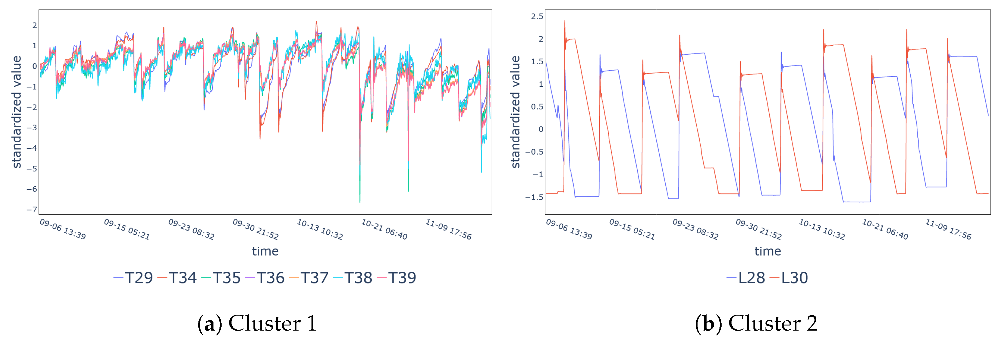
| Cluster 1 | T29, T34-T39 |
| Cluster 2 | L28, L30 |
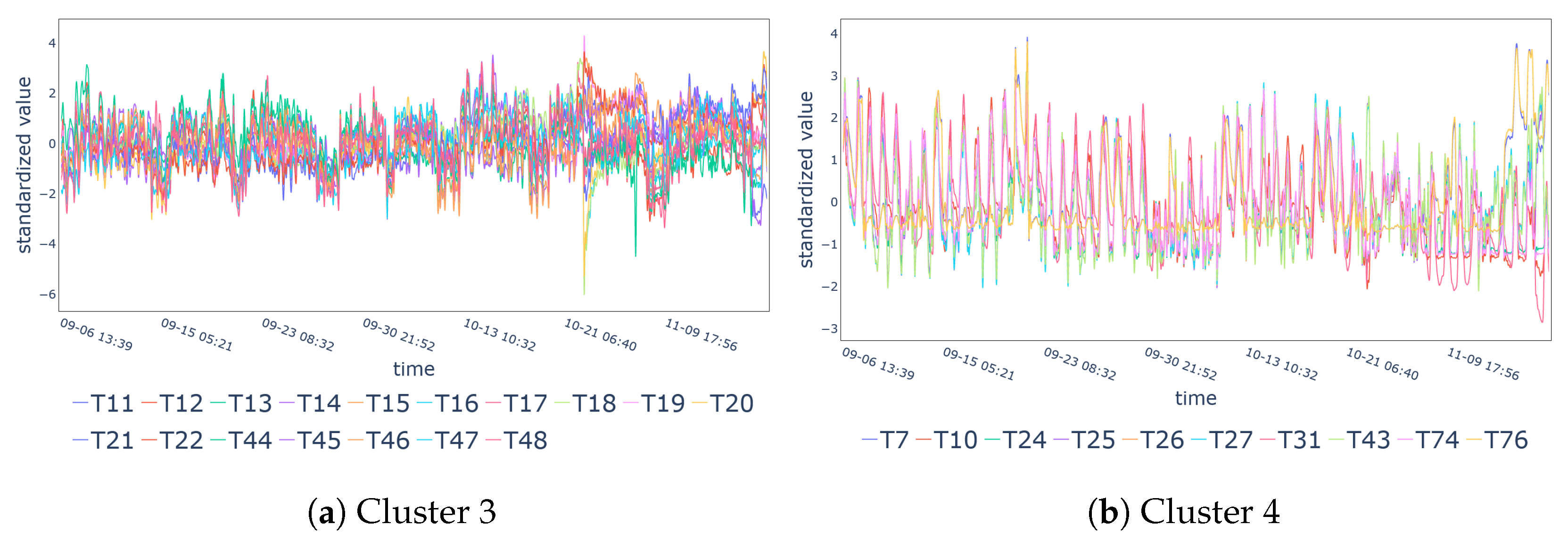
| Cluster 3 | T11-T22, T44-T48 |
| Cluster 4 | T7, T10, T24-T27, T31, T43, T74, T76 |
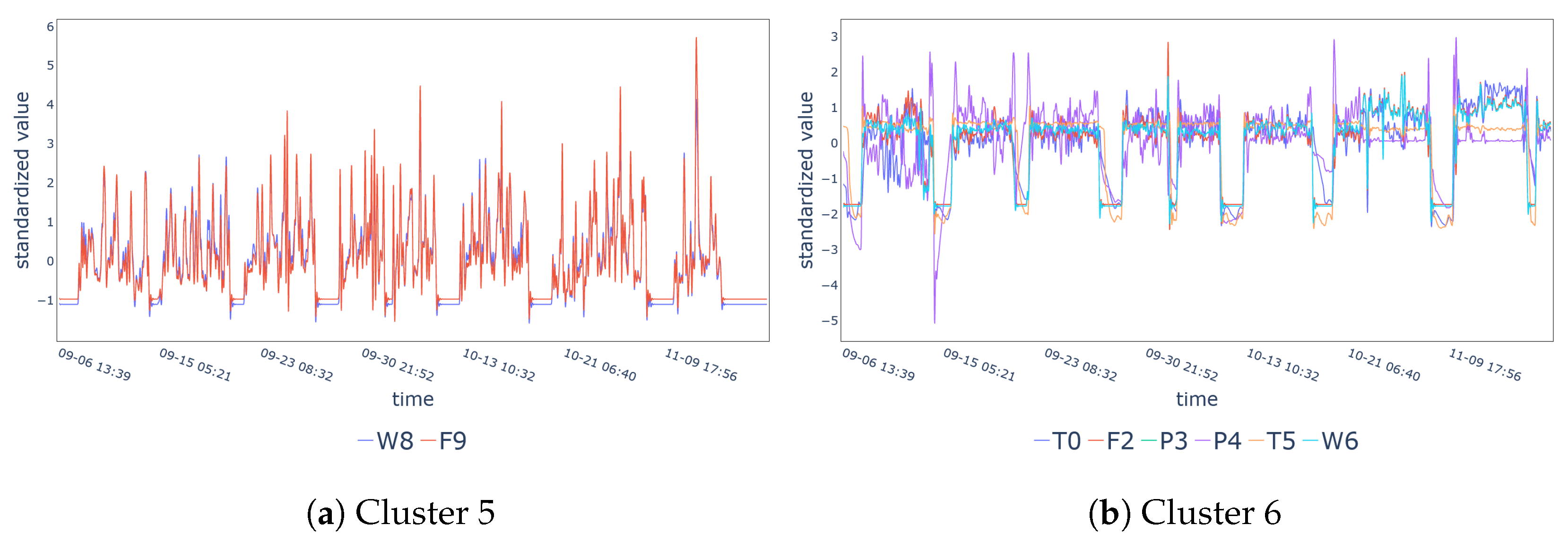
| Cluster 5 | W8, F9 |
| Cluster 6 | T0, F2, P3, P4, T5, W6 |
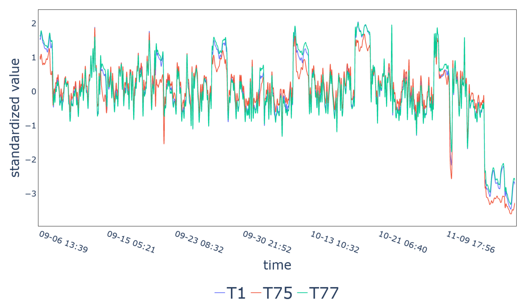
| Cluster 7 | T1, T75, T77 |
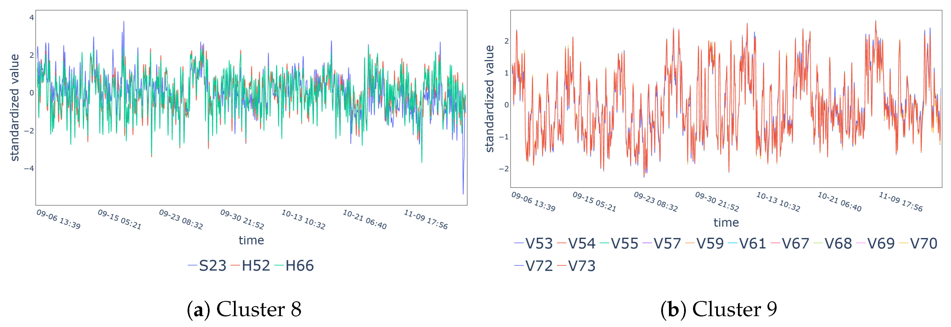
| Cluster 8 | S23, H52, H66 |
| Cluster 9 | V53-V55, V57, V59, V61, V67-V70, V72, V73 |
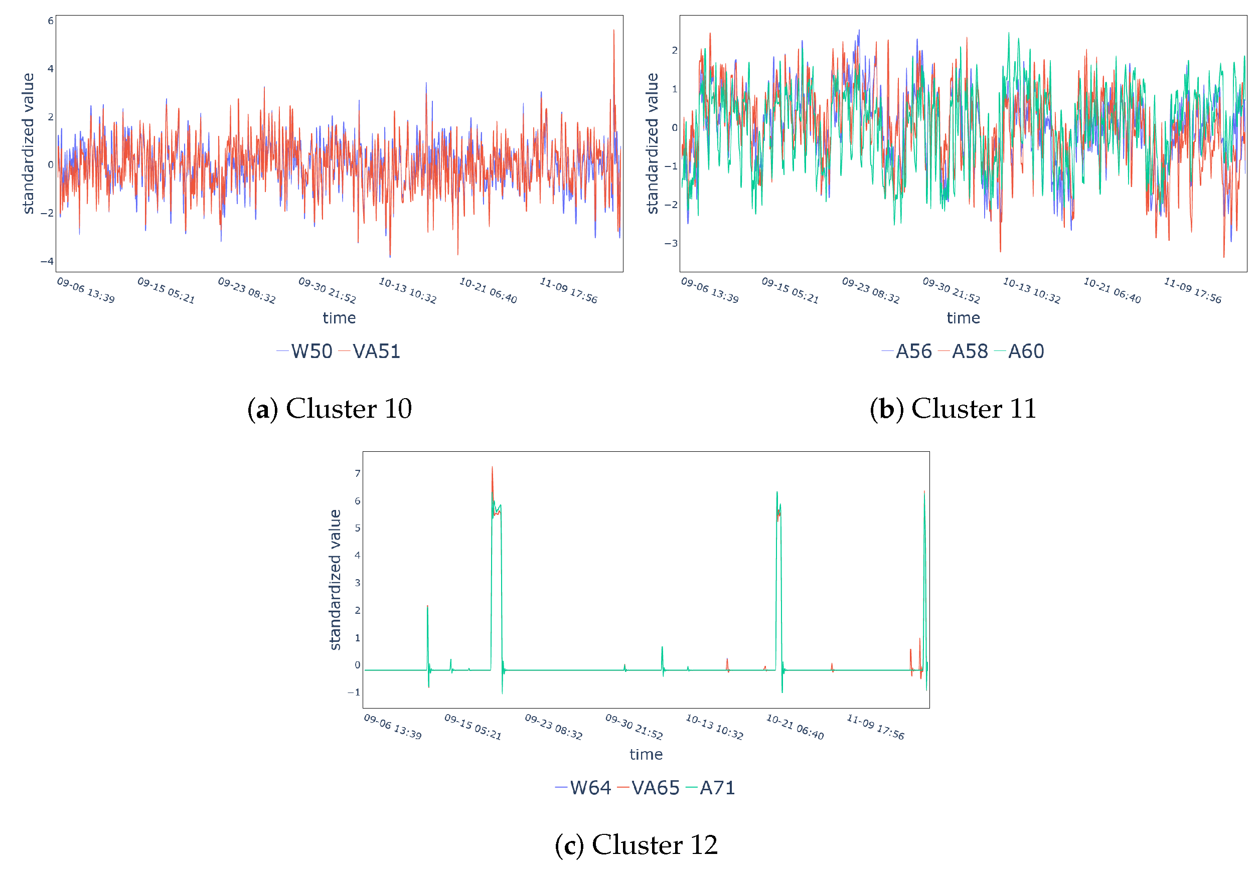
| Cluster 10 | W50, VA51 |
| Cluster 11 | A56, A58, A60 |
| Cluster 12 | W64, VA65, A71 |
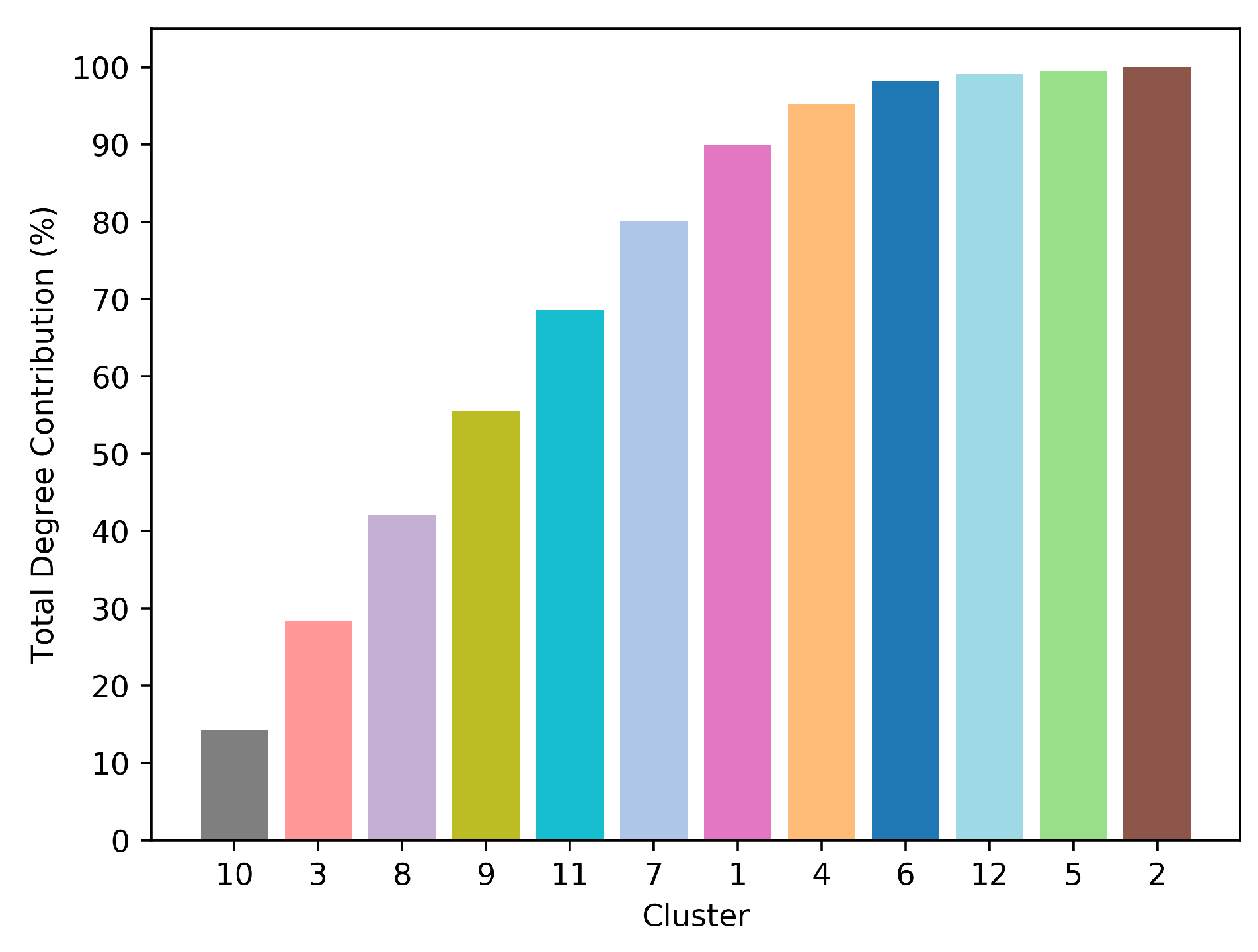
| Cluster ID | Number of Elements | Most Representative Variable ID | Absolute Degree Value | Within Cluster Degree Contribution |
|---|---|---|---|---|
| Cluster 1 | 7 | T38 | 29.44 | 19.51% |
| Cluster 2 | 2 | L30 | 1.00 | 50.00% |
| Cluster 3 | 17 | T19 | 34.62 | 6.61% |
| Cluster 4 | 10 | T43 | 18.20 | 15.34% |
| Cluster 5 | 2 | W8 | 1.00 | 50.00% |
| Cluster 6 | 6 | T0 | 9.03 | 23.50% |
| Cluster 7 | 3 | T75 | 25.83 | 33.96% |
| Cluster 8 | 3 | H66 | 31.06 | 34.18% |
| Cluster 9 | 12 | V72 | 30.91 | 8.70% |
| Cluster 10 | 2 | VA51 | 31.67 | 50.30% |
| Cluster 11 | 3 | A56 | 30.67 | 35.31% |
| Cluster 12 | 3 | W64 | 2.00 | 33.33% |
| Method | Optimal Number of Clusters | RRR | IGR |
|---|---|---|---|
| Proposed approach | 12 | 29.05% | 10.60% |
| Raw-data based | 12 | 9.52% | 8.39% |
| Feature based | 10 | 20.96% | 7.90% |
© 2020 by the authors. Licensee MDPI, Basel, Switzerland. This article is an open access article distributed under the terms and conditions of the Creative Commons Attribution (CC BY) license (http://creativecommons.org/licenses/by/4.0/).
Share and Cite
Bonacina, F.; Miele, E.S.; Corsini, A. Time Series Clustering: A Complex Network-Based Approach for Feature Selection in Multi-Sensor Data. Modelling 2020, 1, 1-21. https://doi.org/10.3390/modelling1010001
Bonacina F, Miele ES, Corsini A. Time Series Clustering: A Complex Network-Based Approach for Feature Selection in Multi-Sensor Data. Modelling. 2020; 1(1):1-21. https://doi.org/10.3390/modelling1010001
Chicago/Turabian StyleBonacina, Fabrizio, Eric Stefan Miele, and Alessandro Corsini. 2020. "Time Series Clustering: A Complex Network-Based Approach for Feature Selection in Multi-Sensor Data" Modelling 1, no. 1: 1-21. https://doi.org/10.3390/modelling1010001