Article

Wavelet-Based Machine Learning Algorithms for Photoacoustic Gas Sensing

1
Physics Department, Novosibirsk State University, Novosibirsk 630090, Russia
2
Institute of Laser Physics, Siberian Branch of the Russian Academy of Sciences, Novosibirsk 630090, Russia
3
Department of Laser Systems, Novosibirsk State Technical University, Novosibirsk 630090, Russia
*
Author to whom correspondence should be addressed.
Optics 2024, 5(2), 207-222; https://doi.org/10.3390/opt5020015
Submission received: 15 February 2024 / Revised: 14 March 2024 / Accepted: 29 March 2024 / Published: 3 April 2024

Abstract

:
The significance of intelligent sensor systems has grown across diverse sectors, including healthcare, environmental surveillance, industrial automation, and security. Photoacoustic gas sensors are a promising type of optical gas sensor due to their high sensitivity, enhanced frequency selectivity, and fast response time. However, they have limitations such as dependence on a high-power light source, a requirement for a high-quality acoustic signal detector, and sensitivity to environmental factors, affecting their accuracy and reliability. Machine learning has great potential in the analysis and interpretation of sensor data as it can identify complex patterns and make accurate predictions based on the available data. We propose a novel approach that utilizes wavelet analysis and neural networks with enhanced architectures to improve the accuracy and sensitivity of photoacoustic gas sensors. Our proposed approach was experimentally tested for methane concentration measurements, showcasing its potential to significantly advance the field of gas detection and analysis, providing more accurate and reliable results.

1. Introduction

Smart sensors and sensor systems have become increasingly important in a wide range of industries due to their ability to gather, process, and provide data in real time. They are critical in various applications, including environmental monitoring, medical diagnosis, and industrial process control, where timely and accurate data are essential for decision making. Among various types of sensors, optical sensors have shown significant potential due to their high sensitivity, selectivity, and fast response time [1]. Photoacoustic gas sensors (PAGSs) have emerged as a promising type of optical gas sensor due to their ability to use light to generate sound waves to detect gas molecules [2,3]. These sensors have several advantages, including high sensitivity and small size, which make them suitable for a range of gas-detection applications. However, PAGSs also have some limitations, such as their dependence on a high-power light source and sensitivity to environmental factors, which can affect the accuracy and robustness of the measurements they perform [4]. Therefore, further comprehensive study of the features of PAGSs is crucial to ensuring their effectiveness and reliability.
Improving the performance of PAGSs can be achieved either by enhancing the characteristics of the equipment and underlying technologies or by developing effective algorithms for interpreting the data produced by PAGSs, which are used to estimate the gas concentration.
Enhancing the acoustic reaction and sensitivity of PAD systems can be achieved by employing more powerful radiation sources [5]. In the visible range, cost-effective and powerful diode lasers can be used for a gas analysis. For example, Yin et al. showed that by employing a diode laser with a wavelength of 447 nm and a power of 3.5 W, a detection sensitivity of 54 pptv for nitrogen dioxide (NO2) was achieved within 1 s of the integration time [6]. In the near-infrared (near-IR) range, diode lasers combined with erbium-doped fiber amplifiers (EDFAs) [7,8] are commonly used as sources of radiation. Nevertheless, visible and near-IR laser diodes are not suitable for detecting all gases. The molecular transitions in the visible and near-IR ranges are at least ten times less intense than the fundamental absorption lines in the mid-IR part of the spectrum [5]. In the mid-IR range, CO and CO2 gas lasers [9], interband cascade lasers (ICLs) [10], along with quantum cascade lasers (QCLs) [11,12] and sources such as optical parametric oscillators (OPOs) and difference frequency generators (DFGs) [13,14] are commonly employed. To increase the average power of mid-IR radiation sources, additional amplification stages are sometimes also used [15,16]. Another method to enhance the sensitivity of gas analyzers involves acoustic wave amplification. To amplify the acoustic wave, various detector resonator configurations are used, such as resonant differential cells [12], Helmholtz cells [17], multipass cells [18], and others [5,18]. To enhance the sensitivity of gas analyzers, different types of acoustic transducers are used, including electret microphones [12], quartz tuning forks (QTF, QEPAS technology) [19], cantilevers (CEPAS technology) [20], and fiber-optic microphones [21].
In recent years, machine learning (ML) has demonstrated great potential in the field of sensor data analysis and interpretation [22,23]. ML algorithms can identify complex patterns in data, learn from them, and use this knowledge to make predictions based on the data. When combined with sensors, ML algorithms can create a powerful analytical tool for accurate detection and analysis. There have been several examples of successful ML applications for sensors reported in the literature, demonstrating the potential for this approach in improving the performance and reliability of sensor systems.
The paper [24] explores the integration of artificial intelligence (AI) in photoacoustic spectroscopy—a powerful and nondestructive technique with broad applications. The focus lies in utilizing AI to achieve the precise and real-time determination of photoacoustic signal parameters, addressing the inverse photoacoustic problem. A feedforward multilayer perceptron network is employed to enhance sensitivity and selectivity, enabling the simultaneous determination of crucial parameters, including the vibrational-to-translational relaxation time and laser beam radius.
In the paper [25], a high-sensitivity gas-detection system for acetylene (C2H2) in the ultra-low concentration range is introduced by using photoacoustic spectroscopy (PAS) by Wang et al. This system employs a novel trapezoid compound ellipsoid resonant photoacoustic cell (TCER-PAC) and a partial least square (PLS) regression algorithm. The study concludes that the proposed PAS system, incorporating TCER-PAC and the PLS algorithm, demonstrates improved detection sensitivity and a lower limit of detection compared to PAS systems based on a trapezoid compound cylindrical resonator, providing a novel solution for high sensitivity and ultra-low concentration detection.
The paper [26] addresses the challenge of selective detection in metal oxide chemiresistive gas sensors with inherent cross-sensitivity. Employing soft computing tools such as Fast Fourier Transform (FFT) and Discrete Wavelet Transform (DWT), the transient response curves of the sensor are processed to extract distinctive features associated with target volatile organic compounds (VOCs). Comparative analysis favors DWT for its superior focus on signal signatures. Extracted features are fed into machine learning algorithms for the qualitative discrimination and quantitative estimation of VOC concentrations. The study emphasizes efficient feature selection, enabling machine learning to achieve an outstanding classification accuracy of 96.84% and precise quantification. The results signify a significant advancement toward automated and real-time gas detection.
The paper [27] reviews the challenges encountered by phase-sensitive optical time-domain reflectometer ( ϕ -OTDR) systems, commonly referred to as distributed acoustic sensing, when monitoring vibrational signals across extensive distances. These systems, operating in complex environments, often face intrusion events and noise interferences, which can affect their overall efficiency. The paper explores several techniques proposed in recent studies to mitigate these challenges, with a specific emphasis on system upgrades, enhancements in data processing, and the integration of ML methods for event classification.
In this study, we propose a novel approach that utilizes a combination of wavelet analysis and neural networks to improve the accuracy and sensitivity of photoacoustic gas sensors. The wavelet analysis method allows for the better detection of gas signals in noisy data, while the use of neural networks with enhanced architectures enables the system to learn complex relationships between the data and the gas concentration. To evaluate the performance of our approach, we conducted laboratory experiments aimed at detecting methane across various concentrations. We then compared our results with those obtained through the conventional Fourier-based method of concentration estimation. Our proposed approach has the potential to provide more accurate and reliable results, resulting in a more efficient gas-detection system. It has the potential to significantly advance the field of gas detection and analysis. The novelty of this work lies in the use of wavelet analysis and machine learning in combination with traditional methods of photoacoustic spectroscopy.

2. Experimental Setup

2.1. Principles of Photoacoustic Gas Sensor

A photoacoustic gas sensor is an optical instrument employed for the detection and quantification of gas concentrations. It achieves this by assessing the magnitude of the acoustic signal produced due to localized heating resulting from the absorption of light by gas molecules. The amplitude of the acoustic signal is directly related to the intensity of the absorbed light as it passes through the gas volume. This intensity is influenced by the gas concentration, the absorption coefficient, and the length of the optical path in an exponential manner. The PAGS comprises two key components: a radiation source that emits light at a wavelength corresponding to the absorption line of the investigated gas and the differential photoacoustic detector (PAD). The PAD has a cavity in which the gas molecules interact with light, and the resonant amplification of the acoustic signal registered by a microphone installed directly in the cavity takes place. The amplitude of the acoustic signal increases significantly if the pulse repetition rate of the radiation source propagating through the gas matches the resonant frequency of the gas cell, resulting in the improved accuracy and sensitivity of the PAGS [2].

2.2. Setup Description

As mentioned above, an important component of PAGSs is the radiation source. As in our previous work [4], a developed optical parametric oscillator (OPO) is used as a radiation source, providing a continuous smooth wavelength tuning in the spectral region of 2.5–4.5 μm, where many gas molecules have their fundamental absorption characteristics. Such a widely tunable source can be utilized for multicomponent gas analysis [28,29].
The foundation of the developed OPO relies on the process of the frequency down-conversion of the Nd:YLF laser in a fan-out MgO:PPLN structure with a domain period that smoothly varies in the range of 27.5–32.5 μm. The experimental setup of the PAGS is sketched in Figure 1. The pump laser has the following characteristics: wavelength—1.053 μm; pulse duration—∼5.3 ns; pulse repetition rate—0.1–4 kHz; linewidth—227 pm; beam quality factor M2—1.4. The nonlinear element was 50 mm long, with an aperture of 20 × 3 mm, and was coated with single-layer antireflection to increase transmission on the signal wave (centered at 1.5 μm), which also resulted in good transmission for the pump at 1.053 μm. The PPLN is maintained at a temperature of T = 40 °C (±0.1 °C) by means of a thermostat based on a Peltier thermoelectric element. For wavelength-tuning purposes, the thermostat is placed in a high-precision motorized linear stage with a 25 mm travel range and 1.25 μm resolutions in full step. A singly resonant OPO was set up with a standard linear cavity consisting of two flat identical input (IC) and output (OC) couplers in a single-pass configuration [30]. Both mirrors were dielectrically coated to reflect highly for the signal wave ( H R > 99 % ) and transparent for the pump and idler waves ( T > 95 % ). An additional dielectric mirror filter was used to minimize the contamination of the pump and signal components of the idler wave (∼3.32 μm) used for the PAD.
The transverse shifting of the PPLN structure relative to the pump laser beam provided tuning of the OPO radiation wavelength in the spectral range of 2.5–4.5 μm with an accuracy setting of ± 0.1 nm. The emission linewidth demonstrated a noticeable decrease as the wavelength increased, ranging from approximately 7.5 cm 1 at 2.5 μm to around 0.6 cm 1 at 4.5 μm. Additionally, at a wavelength of 3.32 μm, the measured emission linewidth was approximately 5.6 ± 0.2 cm 1 . The spectral characteristics of the OPO output radiation were studied by employing an LSA IR laser spectrum analyzer and WS6 wavelength meter (HighFinesse/Angstrom, Tübingen, Germany) with a spectral resolution of 90 pm (12 GHz) and 7 pm (200 MHz), respectively. To carry out experiments to detect methane impurities at various concentrations, the wavelength of OPO radiation was 3.32 μm, which coincides with its maximum absorption peak. In this spectral region, the average output radiation power was ∼35 mW at a pulse repetition rate of 1800 Hz. The average power and pulse energy of the OPO were measured using an Ophir Vega PE-10C (Jerusalem, Israel) power/energy meter positioned in front of the PAD. The spatial characteristics of the idler wave were investigated using a Pirocam IV beam profiling camera (Spiricon, Jerusalem, Israel). To minimize the impact of the power drift of the OPO radiation on the PAD signal (ILP SB RAS, Novosibirsk, Russia), pyrodetector (Pyro MG-30, JSC “NZPP Vostok”, Novosibirsk, Russia) was used. To perform this, a partial reflecting mirror (PRM, R 1 % @ 3.32 μm) in the pyrodetector was placed in the optical path.
During the experiment, OPO radiation was injected into the PAD, where the laser beam interacted with the molecules of the gas under study. The differential PAD is made of a solid aluminum alloy and consists of two parallel acoustic channels (Ø 9 × 90 mm). These channels are separated by a thin partition that is 1 mm thick. Additionally, the PAD includes two buffer cavities (Ø 20 × 8 mm), which are enclosed by flanges. These flanges are equipped with transparent uncoated Zinc Selenide Brewster windows and rubber seals. Gas was transferred through hoses with an inner diameter of Ø2 mm that were installed on the walls of the buffer cavities. The PAD was filled with a gas mixture to reach atmospheric pressure, following which it was sealed. The PAD structure is very close to the cell described in detail in [31]. The detector is also equipped with two electret microphones, one in the center of the acoustic channel. For the precise and accurate balancing of microphone responses, they are connected to the differential amplifier separately per channel. To measure the current lowest resonant frequency, a small-sized piezoelectric sound emitter is housed in the center of one of the acoustic channels opposite of the microphone. The conventional method for determining the resonant frequency of a PAD involves recording a specific segment of the amplitude–frequency characteristics and analyzing the resonance, which is time consuming and introduces measurement errors when the resonant frequency changes. A faster method was used to determine the resonant frequency almost in real time. This method involves applying a series of short voltage pulses to the sound emitter at a repetition frequency close to the expected resonant frequency. The emitter functions as a speaker, stimulating its own acoustic oscillations within the PAD. Subsequently, they are recorded using microphones, and the Fourier transform components are computed within a specified frequency range. The frequency is then determined using the refinement algorithm proposed by E. Jacobsen and P. Kootsookos [32]. This approach enables the measurement of the PAD’s lowest resonant frequency in nearly real time (approximately 0.1 s) with an error margin of around ±0.1 Hz. More detailed information on the measurement technique can be found in [31]. Since the resonant frequency of the PAD is directly related to the speed of sound in the gas mixture it contains, the resonant frequency is significantly influenced by the temperature and composition of the mixture. Hence, the resonant frequency is determined before each measurement. The recorded minimum resonant frequency of the PAD is around 1750 Hz or 1780 Hz when it is filled with air or nitrogen, respectively. The Q-factor of the used detector is Q 40 . The ADC controller receives the electrical signals from the PAD, which allows one to set the required pulse repetition rate for OPO radiation. The alignment of the resonant frequency of the detector with the pulse repetition rate of the radiation source enables a substantial enhancement of the PAD signal [31].

3. Experimental Data and Concentration Estimation Algorithm

3.1. Dataset

The experiments were carried out for a background concentration of methane in the air (about 1.9 ppm) and for two reference gas mixtures based on nitrogen with an admixture of methane ( N 2 + 9.7 and 954 ppm C H 4 ) (1.25, 6.4, and 625.8 mg/m3, respectively). Throughout the experiment, we measured the power of the acoustic signal U m i c r o using a differential PAD and the power of the laser radiation U l a s e r using a photodetector MG-30 with a sampling frequency of 48 kHz. Each measurement lasted for 1 s, and we performed 200 measurements for each concentration. In total, we obtained 600 one-second measurements comprising 48,000 samples for the three concentrations. The algorithms for recovering the concentration of C H 4 described below utilize these measured values as the input data. Figure 2 illustrates an example of the recorded power for the acoustic and optical signals for the three C H 4 concentrations.

3.2. Algorithm for Concentration Estimation Based on Fourier Transform

The basic method for deriving gas concentration values from recorded data relies on the implementation of the Fast Fourier Transform (FFT) algorithm. We begin by applying the FFT to the signals U m i c r o and U l a s e r to transform them into frequency domain representations. Subsequently, we extract the amplitude values F U m i c r o f r and F U l a s e r f r at the resonance frequency f r . Algorithmically, these values are identified as the maximum amplitudes within the entire frequency range. Figure 2 illustrates the FFT outcomes for the three C H 4 concentrations. The figure displays the alignment of the resonance frequency of the acoustic signal from the microphone and the frequency of the optical signal pulses, consistent with the theory of forced oscillations. The signal ratio F U m i c r o f r / F U l a s e r f r adheres to the C H 4 concentration following the Beer–Lambert law. By leveraging several calibration points with known concentrations, it becomes possible to approximate the relationship between the signal ratio and concentration, utilizing this curve for the retrieval of arbitrary concentrations. In this method, the signal U l a s e r serves to compensate for the impact of the wavelength and power drift of the OPO on the PAD signal.
Figure 2. Recorded power for the acoustic and optical signals for a 954 ppm (top), 9.7 ppm (center), and 1.9 ppm (bottom) C H 4 concentration in time domain (left) and frequency domain (right).
Optics 05 00015 g002

4. Problem Formulation and Proposed Solution

The data-processing algorithm, outlined in Section 3, proves effective and applicable when the power of the acoustic signal at the resonant frequency significantly exceeds that at other frequencies. This is typically observed in two scenarios: (i) with relatively high gas concentrations and (ii) when utilizing high-quality sensor components like a microphone or radiation source that avoids introducing significant signal distortions. Furthermore, stable environmental conditions are essential to prevent any influence on the measurement process.
However, in scenarios involving low gas concentrations or the use of inexpensive, low-quality sensor components, the power of the acoustic signal may be comparable to the power of the background noise. In such cases, standard algorithms may lack effectiveness, necessitating advanced approaches. These data interpretation approaches hold the potential to enhance the sensitivity threshold of PAGS, reduce costs through the use of more affordable components, and alleviate sensitivity to environmental factors.
To develop and assess the performance of such approaches, we proposed the following methodology based on collected experimental data. We used the experimental data obtained in the laboratory for all concentrations, which were processed by the basic algorithm, as target values. Subsequently, we generated new datasets for further investigation by introducing additive white Gaussian noise to the experimental signal from the microphone for each of the three concentrations. The noise was uniformly added to the data for each concentration, simulating the degradation of the microphone’s performance. To quantify the amount of added noise, we employed the peak signal-to-noise ratio (PSNR), defined as the ratio of the power of the acoustic signal at the resonant frequency to the average power of the background noise at other frequencies. The obtained noisy signal, denoted as U m i c r o n o i s e , and the signal U l a s e r were utilized as input signals for both the basic and proposed algorithms. To evaluate the performance of both algorithms, we computed metrics (the mean squared error and mean absolute percentage error) between the output of the algorithms on noisy data and the target value F U m i c r o f r / F U l a s e r f r .
In the approach proposed in this study, we suggest performing a wavelet transform of the received signals instead of a Fourier transform. The resulting wavelet representation of signals is then used as input data for neural networks with advanced architectures.

4.1. Wavelet Transform

A wavelet analysis is a powerful method for studying the structure of heterogeneous processes. Currently, wavelets are widely used in pattern recognition, signal processing, and the synthesis of various signals such as speech signals and image analysis, as well as for compressing large amounts of information in many other fields [33]. The one-dimensional wavelet transform involves decomposing a signal into a basis formed by a soliton-like function called a wavelet. Each function in this basis describes the signal in spatial or temporal frequency and its localization in physical space (time) [34]. Unlike the conventional Fourier transform, the one-dimensional wavelet transform yields a two-dimensional representation of the signal in the time–frequency domain. Wavelet transforms can be either discrete or continuous.

4.1.1. Continuous Wavelet Transform

The mathematical expression for the continuous wavelet transform (CWT) involves the convolution of the wavelet function ψ ( t ) with the signal f ( t ) , defined as:
W ψ f ( a , b ) = | a | 1 / 2 f ( t ) ψ * t b a d t ,
where a is the scale coefficient, responsible for wavelet scaling, and b is the shift parameter, responsible for wavelet translation. The choice of the mother wavelet ψ ( t ) is typically guided by the specific task and the information intended to be extracted from the signal.
In our case, working with signals from an optoacoustic gas analyzer, we studied more than twenty wavelet functions and selected the complex Morlet wavelet:
ψ ( t ) = 1 π B e t 2 / B · e j 2 π C t ,
where B represents the bandwidth and C denotes the central frequency. For our task, we selected a bandwidth of one and a central frequency of 1780 Hz. We applied continuous wavelet transform to the recorded time series of the acoustic signal from the microphone and the optical signal from the receiver. Then, we computed the real part of the obtained wavelet coefficients. As a result, we obtained two images of size 50 × 48,000 pixels, corresponding to the signals U m i c r o and U l a s e r . Figure 3 illustrates the characteristic pattern of wavelet coefficients for a gas concentration of 954 ppm.

4.1.2. Wavelet Packet Transform

Wavelet packet transform (WPT) is a variation of the Discrete Wavelet Transform widely employed in digital signal processing for analysis and compression. In the WPT process, the signal is divided into a set of sub-bands using low-pass and high-pass filters. Each sub-band can be further subdivided into two sub-bands. This process continues iteratively until the desired level of decomposition is achieved. Each sub-band contains information about different frequency components of the signal. For instance, low-pass filters capture low-frequency features of the signal, while high-pass filters emphasize high-frequency details. The sub-band corresponding to low frequencies is termed the approximation sub-band (A), while the one obtained using the high-pass filter is called the detail sub-band (D). Figure 4 illustrates the WPT process with a decomposition level of three. Each subsequent sub-band reduces the number of coefficients by approximately half compared to the previous one. The exact reduction depends on the choice of the wavelet function and the method of signal extrapolation at the boundaries.
For decomposing the microphone and laser signals from the optoacoustic gas analyzer, we employed a partial enumeration method and selected a wavelet from the Daubechies family, specifically the fifth order (db5). To improve the decomposition results at the signal boundaries, we applied periodic extrapolation, considering the periodic structure of the original signal. We selected a decomposition level of eight. As a result, from each temporal series with 48,000 measurements, we obtained 256 sub-bands of decomposition. Each sub-band consisted of 196 values. These 256 sub-bands were then organized into a two-dimensional image of size 256 × 196 pixels, accounting for the frequency characteristics of each sub-band. In total, we have two 256 × 196 images, corresponding to the signals U m i c r o and U l a s e r . The preprocessed data result is depicted in Figure 5.
In our investigation, we observed that employing wavelet packet transform instead of continuous wavelet transform leads to a substantial reduction in video card memory requirements, exceeding 40 times. This substantial decrease enhances the speed of prediction calculations and accelerates neural network training. It opens possibilities for exploring deeper convolutional neural network architectures, ultimately improving the accuracy of predictions.

4.2. Neural Networks

Our initial concept was based on employing the outcomes of continuous wavelet transform applied to both acoustic and optical signals. To achieve this, we augmented the initial dataset of 600 measurements to 1200 by duplicating all values twice and then added random additive white Gaussian noise of fixed amplitude to the microphone signal. As a result, we obtained a noisy signal with a parameter PSNR of 5.47, 12.79, and 54.38 dB for concentrations of 1.9, 9.7, and 954 ppm, respectively. The result of the CWT from these signals was used as inputs for a convolution neural network (CNN) with designed architecture, as shown in Figure 6. Thus, the CNN received two wavelet coefficients images, each sized 50 × 48,000 pixels, as the input. Then, a two-dimensional convolution was applied to each image using a shared kernel of size 5 × 5 . The absolute values of the resulting images were then calculated, followed by a max pooling subsampling layer with a size of 8 × 8 . Then, temporal averaging was performed, resulting in seven values remaining for each image. Following this, a linear combination of these values with trainable weights was computed. The output of the convolutional neural network was the ratio of the value corresponding to the acoustic signal to the value corresponding to the optical signal. The target output signal value was the ratio of the amplitudes of signals F [ U m i c r o ] ( f r ) / F [ U l a s e r ] ( f r ) for the noiseless dataset.
To train the neural network, the dataset was divided into training and testing sets, with 840 measurements in the training set and 360 measurements in the testing set. The mean squared error (MSE) was chosen as the loss function. For optimization, we employed the Adam optimization algorithm, adjusting the learning rate dynamically as it reached a plateau. The convolutional neural network was implemented using the PyTorch library 2.1.0 and trained on an Nvidia GTX 1080 Ti graphics card with 11 GB of video memory. The model’s performance evaluation was carried out using the mean absolute percentage error (MAPE) on the predicted values. In the case of the approach employing a continuous wavelet transform in the convolutional neural network, the MAPE error for a concentration of 1.9 ppm was 93%, whereas the Fourier-based approach resulted in an error of 122.3%. The outcomes of the CWT and other approaches are summarized in the Section 5 (Table 3).
While we observed a slight improvement in prediction outcomes, we noted a constraint when training deep neural networks with input images of substantial dimensions derived from a continuous wavelet transform. Moreover, the training and prediction processes using this wavelet transform approach proved to be time consuming. Consequently, we made a decision to shift from a continuous wavelet transform to a wavelet packet transform.

4.2.1. VGG-Net Architecture

One of the most widely adopted configurations of deep convolutional neural networks is known as the VGG architecture. Originating in 2014 at the University of Oxford, its key innovation lies in employing a 3 × 3 convolutional kernel with a stride of one [35,36]. The application of two consecutive 3 × 3 convolutional layers creates a receptive field of size 5 × 5 , requiring only 18 trainable weights. In contrast, using a single 5 × 5 convolutional layer would demand 25 weights. This design choice enables the neural network to achieve greater depth with the same number of trainable weights. The ability to create deeper VGG network models allows for capturing a higher degree of nonlinearity, facilitated by the additional rectified linear unit (ReLU) nonlinearity between layers [37]. We introduce modifications to adapt this architecture for regression tasks, particularly in the structure of the neural network’s output layer and fully connected layers. Additionally, due to limitations in the data volume, we decide to reduce the number of layers and channels in each layer.
Like in the convolutional neural network designed for continuous wavelet transform (Figure 6), two images of noisy signals were employed as the input. These images represented wavelet packet transform maps with dimensions of 256 × 196 pixels. Each image underwent processing by a neural network with uniform weights, generating one output value for the microphone signal and another for the laser signal. Subsequently, the ratio between these outputs was computed. Here, the target value was the noiseless result of the baseline Fourier approach. The training dataset, validation dataset, and test dataset include 9000, 2400, and 600 measurements, respectively. In total, our dataset consisted of 12,000 measurements obtained from 600 noiseless measurements using 20 random noise realizations. The validation set was employed for optimizing model hyperparameters, ensuring that the test set was never used for training.
We employed the open-source library Optuna to tune the hyperparameters and find the optimal architecture for the VGG-type convolutional neural network [38]. The Adam optimization algorithm was chosen as the learning algorithm, and the initial learning rate was optimized in the range from 10 5 to 10 2 . A learning rate reduction algorithm was applied when the validation metric MSE reached a plateau. The hyperparameter “factor”, responsible for reducing the learning rate when reaching a plateau, was selected in the range of 0.1 to 0.9. Additionally, the number of epochs for patience, after which the learning rate was decreased if there was no improvement in accuracy on the validation dataset, was optimized in the range of 2 to 7. The batch size was adjusted within the range of 2 to 64, and the number of epochs was set to 60. The number of channels in each convolutional layer was adjusted from 1 to 32, and the number of neurons in the hidden fully connected layer was chosen within the range of 2 to 16. The optimal architecture of the VGG-type convolutional neural network is presented in Table 1. The applied layers of the neural network are shown in the table in the order in which the image passes through the neural network. A ReLU layer was used as an activation function after each convolutional and fully connected layer.
An efficient optimization algorithm called TPE was used to search for optimal hyperparameters. This algorithm is a variation of the Bayesian optimization method [39]. It operates iteratively, using information about previously evaluated hyperparameters to create a probabilistic model, which is then used to propose the next set of hyperparameters. Additionally, the Hyperband algorithm was employed to early stop unpromising models during the early stages of training. This modern algorithm makes decisions about discarding unsuccessful models based on multiple concurrently computed results. This approach helps avoid discarding models that converge slowly at the beginning but achieve good results in the end [40]. A total of 60 models were analyzed during the optimization process. The optimization was conducted using Tesla V100 GPUs. It took one week of computational time using two GPUs simultaneously to fine tune the hyperparameters.

4.2.2. ResNet Architecture

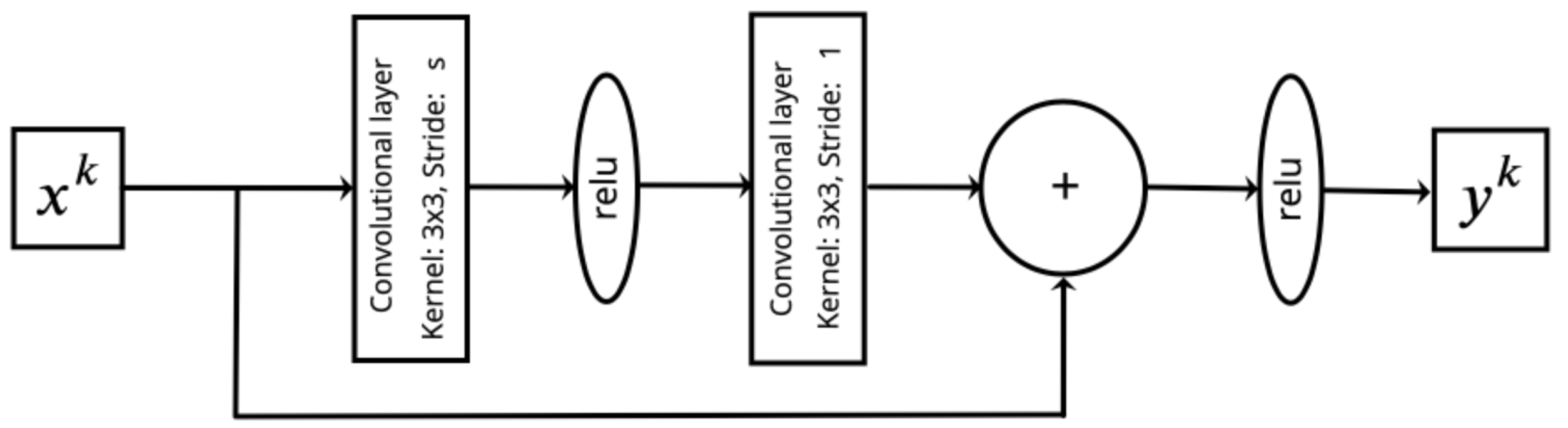
The next architecture selected for deep convolutional neural networks was ResNet. In practice, an accuracy degradation is observed when increasing the depth of neural networks. This decline impacts both the training and test datasets. Importantly, this challenge is not associated with overfitting but rather stems from the inherent difficulties in training deep neural networks [37]. To address the problem of training degradation, the research team at Microsoft Research proposed the concept of deep residual learning, which forms the basis for the ResNet architecture. The residual block serves as the fundamental building block of the residual neural network. The architecture of a single residual block (ResBlock) used for methane concentration restoration from noisy data is shown in Figure 7. One notable feature of this block is the absence of batch normalization. This is because the information is encoded in the signal amplitude. Adding this layer to the investigated architectures resulted in a significant deterioration in the MSE metric.
For the ResNet neural network architecture, similar to the VGG convolutional neural network, the input comprised two wavelet packet transform images of size 256 × 196 pixels derived from a noisy signal. The training, validation, and test dataset comprise 9000, 2400, and 600 measurements, respectively. The Adam algorithm was used for training, with a reduction in the learning rate when the validation MSE metric reached a plateau. The learning rate hyperparameters were tuned in the same range as for VGG. The batch size was optimized in the range of 2 to 64. The number of epochs was set to 60. The number of channels in each residual block was adjusted in the range of 1 to 64. The number of neurons in the hidden fully connected layer was selected in the range of 2 to 32. The optimal ResNet neural network architecture is presented in Table 2. The neural network layers used are shown in the table in the order in which the image passes through the neural network. The ReLU layer was used as an activation function after each convolutional and fully connected layer and also inside the residual blocks. The architecture of residual blocks is shown in Figure 7.
The search for optimal hyperparameters was conducted using the TPE optimization algorithm and the early stopping method Hyperband. A total of 60 models were analyzed. The optimization was conducted using Tesla V100 GPUs. It took two weeks of computational time using two GPUs simultaneously to fine tune the hyperparameters.

5. Results and Discussion

To train the VGG convolutional neural network architecture, as outlined in Table 1, we generated five independent datasets, each containing 12,000 samples, corresponding to five levels of noise applied to the microphone signal (PSNR = −14.75, −6.73, 5.47, 20.16, 33.74 dB for a concentration of 1.9 ppm). Independent training processes were carried out for each noise level, concurrently addressing three investigated concentrations with the same noise amplitude applied to the microphone signal. Consequently, a separate neural network was trained for each noise amplitude level. The results of the test dataset, which was not employed during the training process, are illustrated in Figure 8. This figure presents a comparison between the VGG architecture approach using WPT and the baseline Fourier approach for methane concentrations of 9.7 ppm and 1.9 ppm. The vertical axis denotes the MSE metric in ppm2, while the horizontal axis represents the PSNR parameter.
From Figure 8, we observed that when the peak signal-to-noise ratio of the microphone signal for a concentration of 1.9 ppm is below 20 dB (indicated by the orange dot), a notable reduction in the MSE deviation is observed for the VGG architecture compared to the baseline Fourier-based approach. For these noise levels, the Fourier-based approach struggles to accurately determine the C H 4 concentration, rendering it ineffective. Conversely, convolutional neural network architectures like VGG, utilizing wavelet packet decomposition, maintain the accurate recovery of the methane concentration even at high noise levels (purple and blue dots), showcasing a significantly lower MSE on the test dataset. It should be noted that for the low noise level (red dot), the Fourier-based approach outperforms the VGG accuracy, as the PSNR is still high even for the lowest concentration 1.9 ppm, and the signal does not degrade substantially. Additionally, for VGG, we observed a sharp increase in the MSE for a PSNR less than 0 dB for all concentrations. However, VGG neural networks still demonstrate superior performance compared to the standard Fourier-based approach.
To compare the approaches based on the VGG and ResNet architectures, two neural networks were trained at a noise level of PSNR = 5.47 dB for a methane concentration of 1.9 ppm. This noise level corresponds to the results presented in Figure 8 (green dot). The input data consisted of images obtained using wavelet-packet transform. After predicting the concentration in the test dataset, two graphs were plotted for the metrics MSE and MAPE as a function of the analyzed concentration, as shown in Figure 9.
It can be seen from Figure 9 that the ResNet architecture also demonstrates strong results in predicting concentration and slightly outperforms the results of the VGG architecture for both metrics. Furthermore, we trained a neural network with the same VGG architecture detailed in Table 1. However, for the input images, we utilized images obtained through the Short-Time Fourier Transform (STFT). The target value was also the output of the baseline Fourier approach without noise. The STFT transform was computed using a Hann window. The results are depicted in Figure 9 by the green line. As seen from the figure, this approach performs better than the baseline Fourier-based method but lags behind methods employing wavelet packet transform. The summarized results for the investigated models estimating methane concentration are presented in Table 3.

6. Conclusions

In this study, we introduced a novel methodology that combines wavelet analysis and advanced neural network architectures to enhance the accuracy and sensitivity of photoacoustic gas sensors. The integration of the wavelet analysis proves instrumental in separating gas signals from noisy data, while the utilization of neural networks with advanced architectures enables the system to identify intricate relationships between data patterns and gas concentrations. The experimental validation of our proposed approach focused on methane concentration measurements, presenting a compelling comparison with the conventional Fourier-based concentration-estimation method. We examined widely accepted convolutional neural network architectures such as VGG and ResNet. The results demonstrate the superior performance of our approach, emphasizing its potential to deliver more precise and reliable outcomes in gas detection. According to these results (Table 3), the ResNet architecture with the wavelet packet transform as the input exhibits an almost three-orders-of-magnitude improvement in the MSE for methane concentration estimation at 1.9 ppm compared to the baseline Fourier approach. Significant improvements are also observed in concentration estimation at 9.7 ppm. It is noteworthy that each of the convolutional neural network architectures show enhanced accuracy in estimating low concentrations under high noise conditions.

Author Contributions

Conceptualization, A.K. and A.R.; methodology, A.K., E.E., I.M., N.K., A.B. and A.R.; software, A.K.; investigation, A.K. and E.E.; data curation, A.K., E.E., I.M., N.K., A.B. and A.R.; writing—original draft preparation, A.K.; writing—review and editing, A.K., E.E., I.M., N.K., A.B. and A.R.; supervision, A.B. and A.R.; funding acquisition, A.R. All authors have read and agreed to the published version of the manuscript.

Funding

This research was funded by the Ministry of Education and Science of the Russian Federation (FSUS-2021-0015). The PAGS development and PAD data measurement were funded by the Ministry of Education and Science of the Russian Federation (Project No. FSUS-2020-0036).

Data Availability Statement

The data presented in this study are openly available in FigShare at https://doi.org/10.6084/m9.figshare.25184027 (accessed on 15 February 2024), reference number (https://figshare.com/articles/dataset/NSU_photoacoustic_gas_sensors/25184027 (accessed on 15 February 2024)).

Conflicts of Interest

The authors declare no conflicts of interest. The sponsors had no role in the design of the study; in the collection, analyses, or interpretation of data; in the writing of the manuscript; or in the decision to publish the results.

Abbreviations

The following abbreviations are used in this manuscript:
PAGSPhotoacoustic gas sensor
PADPhotoacoustic detector
OPOOptical parametric oscillator
ICInput coupler
OCOutput coupler
PPLNFan-out periodically poled lithium niobate crystal
PRMPartial reflecting mirror
ADCAnalog-to-digital converter
PCPersonal computer
MLMachine learning
NNNeural network
FFTFast Fourier Transform
WPTWavelet packet transform
CWTContinuous wavelet transform
STFTShort-Time Fourier Transform
MSEMean squared error
MAPEMean absolute percentage error
PSNRPeak signal-to-noise ratio

References

  1. Hodgkinson, J.; Tatam, R.P. Optical gas sensing: A review. Meas. Sci. Technol. 2012, 24, 012004. [Google Scholar] [CrossRef]
  2. Vengerov, M. An Optical-Acoustic Method of Gas Analysis. Nature 1946, 158, 28–29. [Google Scholar] [CrossRef] [PubMed]
  3. Palzer, S. Photoacoustic-Based Gas Sensing: A Review. Sensors 2020, 20, 2745. [Google Scholar] [CrossRef] [PubMed]
  4. Bednyakova, A.; Erushin, E.; Miroshnichenko, I.; Kostyukova, N.; Boyko, A.; Redyuk, A. Enhancing long-term stability of photoacoustic gas sensor using an extremum-seeking control algorithm. Infrared Phys. Technol. 2023, 133, 104821. [Google Scholar] [CrossRef]
  5. Wang, F.; Cheng, Y.; Xue, Q.; Wang, Q.; Liang, R.; Wu, J.; Sun, J.; Zhu, C.; Li, Q. Techniques to enhance the photoacoustic signal for trace gas sensing: A review. Sens. Actuators A Phys. 2022, 345, 113807. [Google Scholar] [CrossRef]
  6. Yin, X.; Dong, L.; Wu, H.; Zheng, H.; Ma, W.; Zhang, L.; Yin, W.; Jia, S.; Tittel, F.K. Sub-ppb nitrogen dioxide detection with a large linear dynamic range by use of a differential photoacoustic cell and a 3.5W blue multimode diode laser. Sens. Actuators B Chem. 2017, 247, 329–335. [Google Scholar] [CrossRef]
  7. Wang, Q.; Wang, Z.; Chang, J.; Ren, W. Fiber-ring laser-based intracavity photoacoustic spectroscopy for trace gas sensing. Opt. Lett. 2017, 42, 2114–2117. [Google Scholar] [CrossRef] [PubMed]
  8. Yin, X.; Dong, L.; Wu, H.; Ma, W.; Zhang, L.; Yin, W.; Xiao, L.; Jia, S.; Tittel, F.K. Ppb-level H2S detection for SF6 decomposition based on a fiber-amplified telecommunication diode laser and a background-gas-induced high-Q photoacoustic cell. Appl. Phys. Lett. 2017, 111, 031109. [Google Scholar] [CrossRef]
  9. Schilt, S.; Thévenaz, L.; Niklès, M.; Emmenegger, L.; Hüglin, C. Ammonia monitoring at trace level using photoacoustic spectroscopy in industrial and environmental applications. Spectrochim. Acta Part A Mol. Biomol. Spectrosc. 2004, 60, 3259–3268. [Google Scholar] [CrossRef]
  10. Tacke, M. New developments and applications of tunable IR lead salt lasers. Infrared Phys. Technol. 1995, 36, 447–463. [Google Scholar] [CrossRef]
  11. Genner, A.; Martín-Mateos, P.; Moser, H.; Lendl, B. A Quantum Cascade Laser-Based Multi-Gas Sensor for Ambient Air Monitoring. Sensors 2020, 20, 1850. [Google Scholar] [CrossRef] [PubMed]
  12. Sherstov, I.; Kolker, D.; Vasiliev, V.; Pavlyuk, A.; Miroshnichenko, M.; Boyko, A.; Kostyukova, N.; Miroshnichenko, I. Laser photo-acoustic methane sensor (7.7 µm) for use at unmanned aerial vehicles. Infrared Phys. Technol. 2023, 133, 104865. [Google Scholar] [CrossRef]
  13. Kostyukova, N.Y.; Kolker, D.B.; Zenov, K.G.; Boyko, A.A.; Starikova, M.K.; Sherstov, I.V.; Karapuzikov, A.A. Mercury thiogallate nanosecond optical parametric oscillator continuously tunable from 4.2 to 10.8 µm. Laser Phys. Lett. 2015, 12, 095401. [Google Scholar] [CrossRef]
  14. Malara, P.; Maddaloni, P.; Gagliardi, G.; Natale, P.D. Combining a difference-frequency source with an off-axis high-finesse cavity for trace-gas monitoring around 3 µm. Opt. Express 2006, 14, 1304–1313. [Google Scholar] [CrossRef] [PubMed]
  15. Arisholm, G.; Nordseth, Ø.; Rustad, G. Optical parametric master oscillator and power amplifier for efficient conversion of high-energy pulses with high beam quality. Opt. Express 2004, 12, 4189–4197. [Google Scholar] [CrossRef] [PubMed]
  16. Yang, Y.P.; Lee, J.Y.; Wang, J. Energetic picosecond 10.2-μm pulses generated in a BGGSe crystal for nonlinear seeding of terawatt-class CO2 amplifiers. Opt. Express 2024, 32, 11182–11192. [Google Scholar] [CrossRef]
  17. Kästle, R.; Sigrist, M.W. Temperature-dependent photoacoustic spectroscopy with a Helmholtz resonator. Appl. Phys. B 1996, 63, 389–397. [Google Scholar] [CrossRef]
  18. Jingsong Li, W.C.; Yu, B. Recent Progress on Infrared Photoacoustic Spectroscopy Techniques. Appl. Spectrosc. Rev. 2011, 46, 440–471. [Google Scholar] [CrossRef]
  19. Patimisco, P.; Spagnolo, V. Quartz-Enhanced Photoacoustic Spectroscopy for Trace Gas Sensing. In Encyclopedia of Analytical Chemistry; John Wiley & Sons, Ltd.: Hoboken, NJ, USA, 2021; pp. 1–17. [Google Scholar] [CrossRef]
  20. Yin, Y.; Ren, D.; Li, C.; Chen, R.; Shi, J. Cantilever-enhanced photoacoustic spectroscopy for gas sensing: A comparison of different displacement detection methods. Photoacoustics 2022, 28, 100423. [Google Scholar] [CrossRef]
  21. Gong, Z.; Gao, T.; Mei, L.; Chen, K.; Chen, Y.; Zhang, B.; Peng, W.; Yu, Q. Ppb-level detection of methane based on an optimized T-type photoacoustic cell and a NIR diode laser. Photoacoustics 2021, 21, 100216. [Google Scholar] [CrossRef]
  22. Chen, Y.N.; Fan, K.C.; Chang, Y.L.; Moriyama, T. Special Issue Review: Artificial Intelligence and Machine Learning Applications in Remote Sensing. Remote Sens. 2023, 15, 569. [Google Scholar] [CrossRef]
  23. Namuduri, S.; Narayanan, B.N.; Davuluru, V.S.P.; Burton, L.; Bhansali, S. Review—Deep Learning Methods for Sensor Based Predictive Maintenance and Future Perspectives for Electrochemical Sensors. J. Electrochem. Soc. 2020, 167, 037552. [Google Scholar] [CrossRef]
  24. Lukic, M.; Cojbasic, Z.; Markushev, D. Artificial Intelligence Application in Photoacoustic of Gases. Facta Univ. Ser. Work. Living Environ. Prot. 2023, 20, 31–44. [Google Scholar] [CrossRef]
  25. Wang, Q.; Xu, S.; Zhu, Z.; Wang, J.; Zou, X.; Zhang, C.; Liu, Q. High sensitivity and ultra-low concentration range photoacoustic spectroscopy based on trapezoid compound ellipsoid resonant photoacoustic cell and partial least square. Photoacoustics 2024, 35, 100583. [Google Scholar] [CrossRef] [PubMed]
  26. Acharyya, S.; Nag, S.; Guha, P.K. Ultra-selective tin oxide-based chemiresistive gas sensor employing signal transform and machine learning techniques. Anal. Chim. Acta 2022, 1217, 339996. [Google Scholar] [CrossRef] [PubMed]
  27. Kandamali, D.F.; Cao, X.; Tian, M.; Jin, Z.; Dong, H.; Yu, K. Machine learning methods for identification and classification ofevents in φ-OTDR systems: A review. Appl. Opt. 2022, 61, 2975–2997. [Google Scholar] [CrossRef] [PubMed]
  28. Kistenev, Y.V.; Borisov, A.V.; Kuzmin, D.A.; Penkova, O.V.; Kostyukova, N.Y.; Karapuzikov, A.A. Exhaled air analysis using wideband wave number tuning range infrared laser photoacoustic spectroscopy. J. Biomed. Opt. 2017, 22, 017002. [Google Scholar] [CrossRef] [PubMed]
  29. Hirschmann, C.; Sinisalo, S.; Uotila, J.; Ojala, S.; Keiski, R. Trace gas detection of benzene, toluene, p-, m- and o-xylene with a compact measurement system using cantilever enhanced photoacoustic spectroscopy and optical parametric oscillator. Vib. Spectrosc. 2013, 68, 170–176. [Google Scholar] [CrossRef]
  30. Kolker, D.; Boyko, A.; Dukhovnikova, N.; Zenov, K.; Sherstov, I.; Starikova, M.; Miroshnichenko, I.; Miroshnichenko, M.; Kashtanov, D.; Kuznetsova, I.; et al. Continuously wavelength tuned optical parametric oscillator based on fan-out periodically poled lithium niobate. Instruments Exp. Tech. 2014, 57, 50–54. [Google Scholar] [CrossRef]
  31. Sherstov, I.; Vasiliev, V.; Goncharenko, A.; Zenov, K.; Pustovalova, R.; Karapuzikov, A. Method for measuring the resonant frequency of photoacoustic detector in the real-time mode. Instruments Exp. Tech. 2016, 59, 749–753. [Google Scholar] [CrossRef]
  32. Jacobsen, E.; Kootsookos, P. Fast, Accurate Frequency Estimators [DSP Tips & Tricks]. IEEE Signal Process. Mag. 2007, 24, 123–125. [Google Scholar] [CrossRef]
  33. Guo, T.; Zhang, T.; Lim, E.; López-Benítez, M.; Ma, F.; Yu, L. A Review of Wavelet Analysis and Its Applications: Challenges and Opportunities. IEEE Access 2022, 10, 58869–58903. [Google Scholar] [CrossRef]
  34. Astafieva, N. Wavelet analysis: Basic theory and some applications. Phys. Usp. 1996, 39, 1085–1108. [Google Scholar] [CrossRef]
  35. Simonyan, K.; Zisserman, A. Very Deep Convolutional Networks for Large-Scale Image Recognition. arXiv 2015, arXiv:1409.1556. [Google Scholar]
  36. Russakovsky, O.; Deng, J.; Su, H.; Krause, J.; Satheesh, S.; Ma, S.; Huang, Z.; Karpathy, A.; Khosla, A.; Bernstein, M.; et al. ImageNet Large Scale Visual Recognition Challenge. arXiv 2015, arXiv:1409.0575. [Google Scholar] [CrossRef]
  37. Goodfellow, I.; Bengio, Y.; Courville, A. Deep Learning; MIT Press: Cambridge, MA, USA, 2016; Available online: http://www.deeplearningbook.org (accessed on 2 September 2023).
  38. Akiba, T.; Sano, S.; Yanase, T.; Ohta, T.; Koyama, M. Optuna: A Next-generation Hyperparameter Optimization Framework. In Proceedings of the 25th ACM SIGKDD International Conference on Knowledge Discovery and Data Mining, Anchorage, AK, USA, 4–8 August 2019. [Google Scholar]
  39. Watanabe, S. Tree-Structured Parzen Estimator: Understanding Its Algorithm Components and Their Roles for Better Empirical Performance. arXiv 2023, arXiv:2304.11127. [Google Scholar]
  40. Li, L.; Jamieson, K.; DeSalvo, G.; Rostamizadeh, A.; Talwalkar, A. Hyperband: A Novel Bandit-Based Approach to Hyperparameter Optimization. arXiv 2018, arXiv:1603.06560. [Google Scholar]
Figure 1. The experimental setup of the developed PAGS system: FI—Faraday isolator, L1 and L2—lenses, IC—input coupler, OC—output coupler, PPLN—fan-out periodically poled lithium niobate crystal, Filter—dielectric mirror filter, Dump—beam dump, PRM—partial reflecting mirror, Pyro—pyrodetector, PAD—photoacoustic detector, ADC—analog-to-digital converter, PC—personal computer.
Optics 05 00015 g001
Figure 3. The wavelet coefficient maps for the microphone signal (left) and the laser signal (right) at a C H 4 concentration of 954 ppm. The color in the image indicates the magnitude of the wavelet coefficients.
Optics 05 00015 g003
Figure 4. Wavelet packet decomposition of a signal with a decomposition level of 3. S represents the original signal, A corresponds to the approximation sub-band, and D corresponds to the detail sub-band.
Optics 05 00015 g004
Figure 5. Wavelet packet transform for the microphone signal at C H 4 concentration of 954 ppm.
Optics 05 00015 g005
Figure 6. The architecture of the convolutional neural network for continuous wavelet transform as input data.
Optics 05 00015 g006
Figure 7. The architecture of a residual block (ResBlock). The shift magnitude s of the first convolutional layer can vary. x ( k ) is the input vector and y ( k ) is the output of the residual block.
Optics 05 00015 g007
Figure 8. Comparison between the VGG architecture approach using WPT (colored dots) and the baseline Fourier approach (black line). The left graph displays the results for a methane concentration of 9.7 ppm, while the right graph exhibits the results for 1.9 ppm.
Optics 05 00015 g008
Figure 9. Comparison of the VGG architecture approach (purple line) and ResNet architecture approach (red line) using WPT. The black line represents the baseline Fourier approach, and the green line represents the VGG architecture with STFT.
Optics 05 00015 g009
Table 1. The optimal VGG-type architecture for methane concentration estimation.
Layer
Type
Kernel
Size
Number of
Channels
Stride
Kernel
Output
Size
Number of
Weights
Input--- 256 × 196 -
Convolutional 3 × 3 16 1 × 1 256 × 196 160
Convolutional 3 × 3 16 1 × 1 256 × 196 2320
Max pooling 3 × 3 - 3 × 3 86 × 66 -
Convolutional 3 × 3 16 1 × 1 86 × 66 2320
Max pooling 3 × 3 - 3 × 3 29 × 22 -
Convolutional 3 × 3 16 1 × 1 29 × 22 2320
Max pooling 29 × 22 -- 1 × 1 -
Flatten Layer
Layer TypeNumber of NeuronsNonlinearityNumber of Weights
Fully connected7relu119
Output1-8
Table 2. The optimal ResNet-type architecture for methane concentration estimation.
Layer
Type
Kernel
Size
Number of
Channels
Stride
Kernel
Output
Size
Number of
Weights
Input--- 256 × 196 -
Convolutional 7 × 7 32 2 × 2 128 × 98 1600
Max pooling 3 × 3 - 2 × 2 64 × 49 -
ResBlock 3 × 3 32 1 × 1 64 × 49 18,496
ResBlock 3 × 3 16 2 × 2 32 × 25 9776
ResBlock 3 × 3 16 1 × 1 32 × 25 4640
ResBlock 3 × 3 2 2 × 2 16 × 13 614
ResBlock 3 × 3 2 1 × 1 16 × 13 76
Avg pooling 16 13 -- 1 1 -
Flatten Layer
Layer TypeNumber of NeuronsNonlinearityNumber of Weights
Fully connected7relu21
Output1-8
Table 3. Comparison of different convolutional neural network architectures for methane concentration estimation with a PSNR of 5.47 dB for a concentration of 1.9 ppm.
ModelConcentration 1.9 ppmConcentration 9.7 ppm
ArchitectureProcessing MethodMSE,ppm2MAPE, %MSE,ppm2MAPE, %
-FFT6.401122.36.25320.3
CNNCWT3.58993.06.53820.6
VGGSTFT0.0318.80.2323.8
VGGWPT0.0135.50.1373.0
ResNetWPT0.0115.40.0982.6
Disclaimer/Publisher’s Note: The statements, opinions and data contained in all publications are solely those of the individual author(s) and contributor(s) and not of MDPI and/or the editor(s). MDPI and/or the editor(s) disclaim responsibility for any injury to people or property resulting from any ideas, methods, instructions or products referred to in the content.

