Image Haziness Contrast Metric Describing Optical Scattering Depth

Abstract

Contrast is not uniquely defined in the literature. There is a need for a contrast measure that scales linearly and monotonically with the optical scattering depth of a translucent scattering layer that covers an object. Here, we address this issue by proposing an image contrast metric, which we call the Haziness contrast metric. In its essence, the Haziness contrast compares normalized histograms of multiple blocks of the image, a pair at a time. Subsequently, we test several prominent contrast metrics in the literature, as well as the new one, by using milk as a scattering medium in front of an object to simulate a decline in image contrast. Compared to other contrast metrics, the Haziness contrast metric is monotonic and close to linear for increasing density of the scattering material, compared with other metrics in the literature. The Haziness contrast has a wider dynamic range, and it correctly predicts the order of scattering depth for all the channels in the RGB image. Utilization of the metric to evaluate the performance assessment of dehazing algorithms is also suggested.

1. Introduction

Establishing a contrast of an image is a classical problem in image processing. The challenge is somewhat ill-posed, and several approaches to this issue have been proposed in the past. One of the oldest ways to calculate contrast is the Weber contrast, which is appropriate for a uniform foreground and a uniform background image [1]. For images with patterns, in which the bright and dark intensities occupy similar fractions of the image, the Michelson contrast [2]. is more appropriate. Another traditional way to define contrast is the root-mean-square (RMS) of the image [3]. Modern contrast scales successfully measure contrast for image optimization and image haziness removal [4,5,6,7], which require low levels of scattering, as shown in the top row of Figure 1. Contrast metrics with better sensitivity, such as the image Histogram Spread [8] presents better contrast discrimination also at high haziness levels. More recently, computationally sophisticated contrast metrics have been developed and studied, including psychophysical contrast measurements [9] and with machine learning algorithms to select the best dehazing of an image [10]. However, the literature lacks a metric that changes monotonically with the haziness or fogginess occluding an object, which is insensitive to changes like image histogram equalization, min-max contrast correction, and brightness correction and is nearly linear for a large dynamic range of optical scattering depth.

In media where scattering plays a major role, optical scattering depth (OD) grows linearly with both optical path length (l) and with the scattering coefficient ($\mu$): $OD=\mu$L. If the medium is air or water, for example, light rays are absorbed and scattered using the medium and other materials dissolved in it. The absorption and scattering depend both on the wavelength and the size distribution of the suspended particles [11]. The optical scattering depth depends specifically on the scattering component of the optical depth. Scattering media between the observer and an object causes the contrast of the image of the object to decrease. The definition we use for contrast is the one where the reduction in contrast in the features of a scene is proportional to the optical scattering depth between the observer and the object.

In this paper, we present a quantitative way of measuring contrast that is nearly linear for a large dynamic range of optical scattering depth. This scale, which we call the Haziness scale, fulfills the requirement of linearity for increasing density of the scattering material and works well over a dynamic range wider than possible for other contrast scales shown in the literature. To test the proposed metric in a controlled environment, use actual photographs where milk is added along the optical path to simulate a decline in image contrast due to the scattering of light with the milk constituents (Figure 1). Later, we apply the Haziness metric to quantify and compare some defogging algorithms from the literature. Applications of the Haziness metric include, for example, the study of optical coherence tomography (OCT), eye retina images, measurement of the amount of fat present in milk, and eye fundus photography.

The rest of the article is organized as follows. In Section 2, we will describe several prominent metrics from the literature. In Section 3, we define our proposed Haziness scale; the relevant imaging experiments are conducted in Section 4. We present our results and discussion in Section 5 using the images we have produced and images from the literature, finishing with relevant conclusions in Section 6.

2. Prior Art

The following section provides some details regarding existing popular contrast measures.

2.1. Weber Contrast

Weber contrast [1] is one of the oldest contrast metrics, used to measure the contrast when there is a uniform background and a well-defined target: $Weber=(I-I_b)/I_b$, where $I$ and $I_b$ represent target and background luminances, respectively. However, this definition is not appropriate for a global contrast measurement, since very bright or dark spots would determine the contrast of the entire image. Thus, we have modified the conventional definition to handle grayscale images, by changing the denominator to the average luminance of the image, denoted with $\overline{I}$:

$$Weber=\frac{I-I_b}{\overline{I}},$$

(1)

where $I$ is measured for each pixel and $I_b$ represents the darkest pixel of the grayscale image.

2.2. Michelson Contrast

The Michelson Contrast [1,2] can be defined for a grayscale image as

$$Michelson=\frac{I_{max}-I_{min}}{I_{max}+I_{min}},$$

(2)

where $I_{max}$ and $I_{min }$ are the maximal and minimal luminance values of the image. The Michelson contrast is a metric originally used for images with sinusoidal patterns and is a poor measure for complex images.

2.3. Root Mean Square Contrast

The root mean square (RMS) contrast has been related to human perception [12,13] and is widely used as an image summary statistic [3]. The RMS contrast is defined as

$$RMS={\left[\frac{1}{n} \sum _{i=1}^n{\left(x_i-\underset{\_}{\overline{x}}\right)}^2\right]}^{\frac{1}{2}},$$

(3)

where $x_i\in \left[0, 1\right]$ is a normalized gray-level value, $\overline{x}=\frac{1}{n} {\sum }_{i=1}^n{x}_i$ is the mean gray level, and $n$ is the number of pixels in the image. For color images, RMS is calculated separately for each channel.

2.4. Histogram Spread

Histogram Spread (HS) is defined as the interquartile range of the cumulative histogram divided by the pixel value range [8]: We first take the image’s histogram and normalize it such that its sum is 1. Next, we calculate the positions of the first and third quartiles of the cumulative histogram and take the difference from those positions. Histogram Spread is this difference divided by the pixel range, the difference between the highest and lowest possible intensity for the pixels:

$$HS=\frac{Q_3-Q_1}{p_{max}-p_{min}},$$

(4)

where $Q_n$ is the $n$-th quartile and $p_{max}$ and $p_{min}$ are the maximum and minimum values for the pixels, respectively. Histogram Spread has a range of values from 0 to 1.

2.5. Rizzi

A method suggested by Rizzi et al. [14], estimates global and local components of contrast. The algorithm works as follows: First, it under-samples the original image, then the under-sampled images are transformed to CIELAB color space [15]. Afterwards, it calculates the mean value of the 8-Neighborhood local contrast for each pixel in the L* channel, and finally sums the averages of each of the under-sampled images to obtain a global measure.

3. Haziness Metric Definition

Here, we describe our proposed metric. When a uniform scattering medium is added to a scene, the scattering light contribution is added to all regions of an image of such scene. To define the Haziness contrast metric, we take advantage of the fact that an increase in scattering within a scene increases similarity of histograms of any two small subregions of the image, on average. We normalize the histogram of each small subregion to ensure invariance to image renormalizations such as full-image histogram equalization, brightness, or contrast correction. The Haziness metric is determined using the average difference between pairs of normalized histograms of small image patches. Figure 2 shows the general idea: as the haziness in the image increases, the histograms of two different regions of the image become more similar. The unitary area normalized histograms are represented by vectors $\overrightarrow{H_i}$ and $\overrightarrow{H_j}$. The Haziness contrast metric is inspired by the foreground to background histogram contrast as described in [16] (see also the preliminary and relevant analysis in [17,18]). One of the several differences here is that the two blocks, $i$ and $j,$ are at random positions in the image for the Haziness contrast metric, and thus, there is no need to manually select the foreground and background.

The Haziness contrast metric is calculated as follows. Two random image blocks, $i$ and $j,$ of $s\times s$ pixels are sampled. The $s\times s$ pixels image blocks have area-normalized histograms $\overrightarrow{H_i}$ and $\overrightarrow{H_j}$, respectively, where the vectors $\overrightarrow{H}$ represent the values of each image block. By area-normalized we mean that the sum of their entries is 1, that is, $\Vert \overrightarrow{H_i} {\Vert }_1=1$, where $\Vert \cdot {\Vert }_1$ is the taxicab $l_1$-norm [19]. Each histogram vector, $\overrightarrow{H_i}$ and $\overrightarrow{H_j}$, has $2^b$ entries, where $b$ is the bit-depth of the image (e.g., 8-bit). With these definitions we have

$$Haziness={⟨\frac{{‖\overrightarrow{H_i}-\overrightarrow{H_j}‖}_1}{{‖\overrightarrow{H_i}+\overrightarrow{H_j}‖}_1}⟩}_N,$$

(5)

where $⟨\cdot ⟩$ represents the average of $N$ random pairs of blocks ($N\gg 1)$.

As can be seen from the definition, a minor disadvantage of the metric is the existence of two tuning parameters: the number and size of patches. The number of patches N must be enough for the haziness contrast value to converge. For N ~ 1000 the Haziness metric converges to within 1% of a finite constant value for the image. In our analysis, we used N = 10⁴. For the metric to represent haziness, s must be small compared to the image’s features. For s of the order of the size of the image, the s × s image blocks are almost identical, resulting in similar histograms for the different patches, and the Haziness contrast metric value will tend to zero. Measures at a granular level (s < 10) provide a more monotonic behavior for the Haziness metric as a function of increasing optical scattering. After experimentation we chose and recommended s = 2 because this is the minimum size for a square patch that can still produce a non-trivial histogram $\overrightarrow{H}$. Although a very small s goes against our initial intuition (Figure 2), small histograms are compensated by the large N, represent a better map of the local structure of the image, and thus maximize monotonicity of haziness contrast as a function of the optical scattering level. 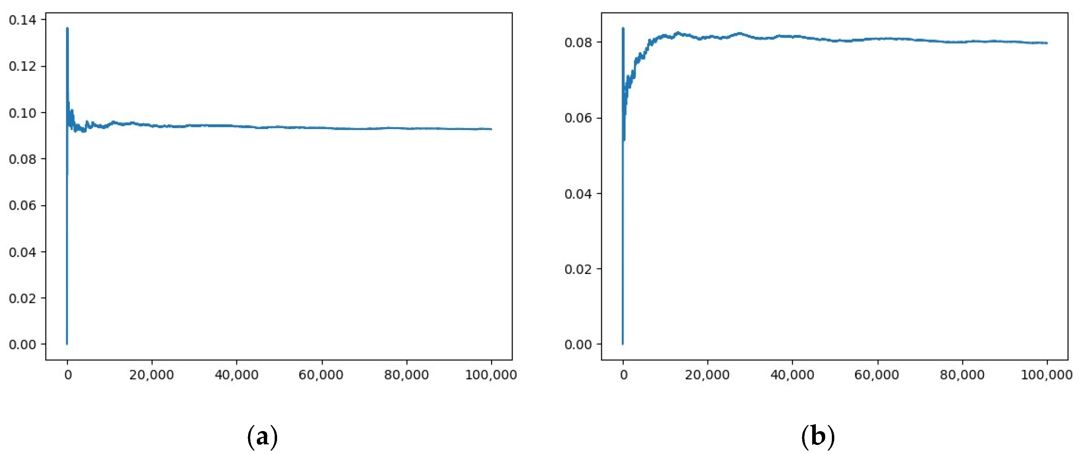Appendix A shows empirical examples where the standard deviation of haziness converges to a finite value, which is a sufficient but not necessary condition for the haziness mean value to converge. The standard deviation of the Haziness metric can be used to further characterize the image, but such analysis is out of the scope of the current study.

4. Image Acquisition Experiment

Instead of using digital image processing techniques to change the image, such as Gaussian blur, we decided to take a physical, empirical approach. To test the performance of the Haziness metric, we simulated fogginess or haziness using water and milk. Starting with a clean image, we gradually added more milk, increasing the optical scattering depth, and thus, the opacity of the image.

Photographs were taken using the main camera of a mobile phone. The phone was mounted above a container filled initially with water and positioned above an image. A photo was taken for every 5 mL of milk added to the water container, with a pipette, up to 35 mL to simulate a linear decline in contrast, or similarly, an increase in the amount of fog in the image. The images have a size of 1188 by 1446 pixels and a resolution of 96 dpi, in JPEG format.

The conversion from RGB to grayscale (luma) used OpenCV’s [20] formula $Y=0.299R+0.587G+0.114B$, where the relative weights are based on the spectral sensitivity of the human eye. All details are provided on GitHub in the Python scripts and data used to produce the results of this paper [21].

5. Results and Discussion

In this section, we focus on how the metrics correlate with optical scattering depth, for each RGB channel, and in grayscale. The purpose of the Haziness metric is to quantify the contrast in the image, thus it does not identify the haze nor tries to de-haze the images, as some previous studies have done [4,5,6,7]. The scales were analyzed in two ways: in grayscale, and in RGB with each channel treated separately. In this study, we do not consider the polarization caused by scattering [22], neither we have tried polarized imaging techniques.

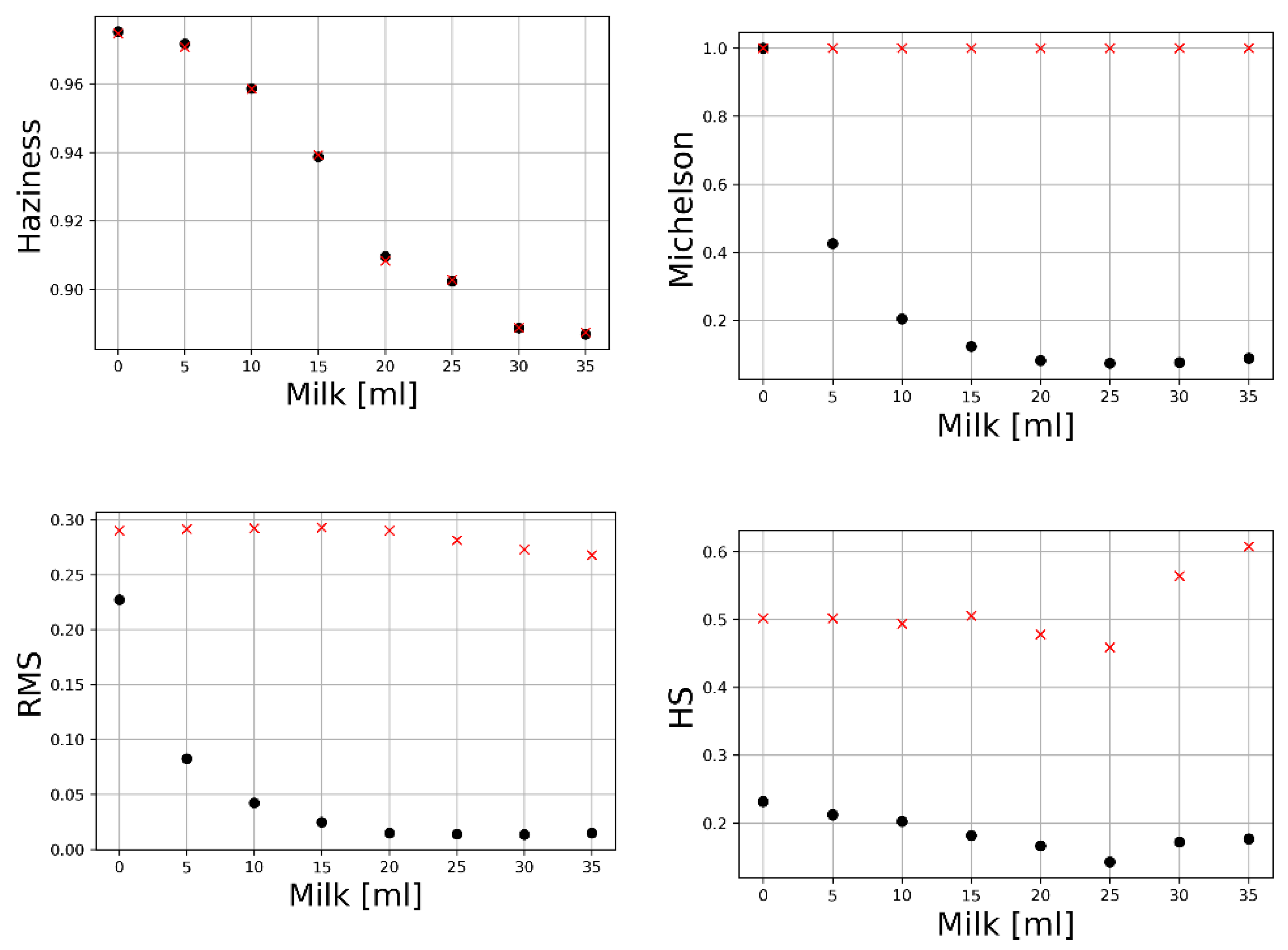
The application of the various contrast metrics discussed earlier in this paper is shown in Figure 3. A log scale is used to better discriminate the scattering for higher depths. The red, green, and blue colors represent the respective RGB channels, and the black line represents the grayscale measurements. We notice that the new Haziness metric (Figure 3a) is monotonic and quasi-linear as a function of increasing scattering medium concentration. None of the other metrics showed a perfectly linear behavior. Moreover, the Haziness measurement has a wider dynamic range, and it is possible to identify which color is most scattered even for a high amount of added scatterer (milk). In the case of grayscale images, the Haziness values are also monotonic and quasi-linear, as the concentration of milk increases, the range of color diminishes, and the contrast declines. For Michelson (Figure 3b) and RMS (Figure 3c) metrics, the slope of the curve for low milk concentrations is high, and we can see a difference as milk is added to the bowl of water. However, from 20 mL and onward, there are no significant differences, both for the RGB values and for the grayscale. The Michelson and RMS measurements are monotonic but possess poor discrimination power for high scattering depths. The graphs for the Weber and Rizzi metrics were omitted here (they will be shown in Figure 3) since their behavior is very similar to RMS and Michelson. The Histogram Spread metric (Figure 2d) presents a non-linear behavior and fails to show lower scattering for the red light, as physically expected. Despite the histogram spread showing good discrimination for the different colors, the monotonicity is poor, with somewhat better results for the blue channel.

For a better comparison of all the studied metrics, we use min-max normalization to present all the results for grayscale images on the same axes (Figure 4). The RMS, Michelson, Weber, and Rizzi metrics all have similar nonlinear monotonic curves. The Haziness metric (Figure 3a) shows a more adequate behavior than the others.

In general, we interpret the Haziness such that the larger its value (the closer it is to one), the better the image contrast. A possible interpretation for the different behavior observed for distinct RGB colors is the distinct amount of scattering each color demonstrates., e.g., in Figure 3a, the blue color has lower values than red (except in the last measurement) since blue scatters more than red. We speculate that the low amount of red and the excess of green color in the image used as a sample (Figure 1) might explain the exceptional Haziness metric behavior, especially for the green channel and at high optical scattering depths.

An interesting follow-up question would be how the metrics behave when we change the contrast and brightness and when we apply a histogram equalization. In other words, the images are modified via image processing tools, and the degree to which the studied metrics are invariant under transformations is observed. To reach that goal, the contrast and brightness of the images of Figure 1 were manipulated via the Pillow library in Python [23], within the ranges of [0.8, 1.2] in both contrast and brightness, in 0.1 increments (with factors of 1.0 corresponding to the original images).

Figure 5 shows the behavior of the metrics when we change the contrast. Michelson and RMS metrics vary monotonically with the variation in contrast, with higher contrast values translating into higher metric values. The Histogram Spread demonstrates a non-linear behavior, while the Haziness metric is, to a large extent, monotonic.

Figure 6 shows the behavior of the metrics when we change the brightness. The RMS metric varies linearly with the variation in brightness, with higher brightness values translating into higher metric values. The Michelson metric is not affected by changes in brightness. The Histogram Spread has a non-linear behavior. The Haziness metric is monotonic and demonstrates a higher discrimination in the values when the brightness is low and the density of milk is high (above 15 mL, in our experiment).

Histogram equalization is another common and useful contrast adjustment method in image processing. We applied the equalizeHist method of OpenCV [20] to the images and observed the behavior of the different metrics. As can be seen in Figure 7, the Haziness metric is robust for histogram equalization, while Michelson, RMS, and Histogram Spread metrics are equalization-sensitive.

It is also of interest to observe the behavior of the different metrics on the ubiquitous Lena test image, with contrast and brightness variations as above. Figure 8 shows how changes in brightness and contrast on Lena affect the metrics. Haziness varies less than the other metrics, which is good.

Another interesting area of study in image processing, and certainly related to the current paper, is image dehazing. Properly removing haze can naturally increase the visibility of the scene. We now compare two single image dehaze algorithms by Fatal [24] and Berman et al. [25], while checking whether the algorithms improved or worsened the Haziness values between the original images (taken from [26,27]; see Figure 9) and the dehazed ones. A higher Haziness metric value represents a better contrast image, with better visibility.

Table 1. Haziness values for the original images and Berman et al. and Fattal dehazing algorithms, with their respective p-values. Whether the Haziness values for the output images increased or decreased after the dehaze algorithm and their p-values, (+) represents if the value increased and (−) if the value decreased. A higher value of the Haziness metrics means better (higher) contrast. Here, the standard uncertainty is determined from ${10}^2$ runs of the Haziness metric with $\mathrm{N}={10}^3$.

	Original	Std	Fattal [24]	p-Value	Berman et al. [25]	p-Value
cityscape	0.967	0.0003	0.978 (+)	8 × 10−11	0.983 (+)	4 × 10−11
forest	0.974	0.0003	0.965 (−)	2 × 10−5	0.979 (+)	4 × 10−4
pumpkins	0.980	0.0002	0.975 (−)	4 × 10−4	0.979 (−)	0.27
train	0.972	0.0003	0.971 (−)	0.27	0.975 (+)	2× 10−2

summarizes the results for the Berman and Fattal algorithms, with their respective mean, standard deviations, and p-values for the Haziness metrics; 100 runs of the Haziness metric with N = 1000 were performed in each case. The table also shows whether the Haziness values for the output images increased (+) or decreased (−) from the original image. Overall, the values for Berman increased, except for the image of the pumpkin (where the decrease was very slight). However, the Haziness metric before and after application of Berman’s dehazing is statistically inconclusive (p-value > 5%) for the pumpkins’ image correction. Meanwhile, in Fattal’s algorithm, the Haziness metric (contrast) increased (improved) only for cityscape images. As argued in [25], Fattal’s method leaves some haze and artifacts in the results, and generally, the Berman non-local image dehazing method produces superior results. Notice that the Haziness metric automatically determined Berman’s algorithm to be superior to Fattal’s algorithm, without room for subjectivity.

6. Conclusions

The proposed Haziness metric is monotonic and closer to linear as a function of the optical scattering depth, compared with other metrics in the literature. It also has a wider dynamic range, being able to quantify haziness levels at scattering levels at least two times deeper than existing metrics. Finally, the Haziness metric correctly predicts the correct order of scattering depth for the red, green, and blue channels of the RGB image. An application of the metric for performance comparison of dehazing algorithms looks promising as well.

References

1. Peli, E. Contrast in complex images. J. Opt. Soc. Am. A 1990, 7, 2032–2040. [Google Scholar] [CrossRef] [PubMed]
2. Michelson, A.A. Studies in Optics; Dover Publications: New York, NY, USA, 1995. [Google Scholar]
3. Pavel, M.; Sperling, G.; Riedl, T.; Vanderbeek, A. Limits of visual communication: The effect of signal-to-noise ratio on the intelligibility of American Sign Language. J. Opt. Soc. Am. A 1987, 4, 2355–2365. [Google Scholar] [CrossRef] [PubMed]
4. Kim, J.-H.; Jang, W.-D.; Sim, J.-Y.; Kim, C.-S. Optimized contrast enhancement for real-time image and video dehazing. J. Vis. Commun. Image Represent. 2013, 24, 410–425. [Google Scholar] [CrossRef]
5. Tan, R.T. Visibility in bad weather from a single image. In Proceedings of the 2008 IEEE Conference on Computer Vision and Pattern Recognition, Anchorage, AK, USA, 23–28 June 2008; pp. 1–8. [Google Scholar] [CrossRef]
6. Narasimhan, S.; Nayar, S. Contrast restoration of weather degraded images. IEEE Trans. Pattern Anal. Mach. Intell. 2003, 25, 713–724. [Google Scholar] [CrossRef]
7. He, K.; Sun, J.; Tang, X. Single Image Haze Removal Using Dark Channel Prior. IEEE Trans. Pattern Anal. Mach. Intell. 2011, 33, 2341–2353. [Google Scholar] [CrossRef] [PubMed]
8. Tripathi, A.K.; Mukhopadhyay, S.; Dhara, A.K. Performance metrics for image contrast. In Proceedings of the 2011 International Conference on Image Information Processing, Shimla, India, 3–5 November 2011; pp. 1–4. [Google Scholar] [CrossRef]
9. Min, X.; Zhai, G.; Gu, K.; Yang, X.; Guan, X. Objective Quality Evaluation of Dehazed Images. IEEE Trans. Intell. Transp. Syst. 2018, 20, 2879–2892. [Google Scholar] [CrossRef]
10. Santra, S.; Mondal, R.; Chanda, B. Learning a Patch Quality Comparator for Single Image Dehazing. IEEE Trans. Image Process. 2018, 27, 4598–4607. [Google Scholar] [CrossRef] [PubMed]
11. Amer, K.O.; Elbouz, M.; Alfalou, A.; Brosseau, C.; Hajjami, J. Enhancing underwater optical imaging by using a low-pass polarization filter. Opt. Express 2019, 27, 621–643. [Google Scholar] [CrossRef] [PubMed]
12. Bex, P.J.; Solomon, S.G.; Dakin, S.C. Contrast sensitivity in natural scenes depends on edge as well as spatial frequency structure. J. Vis. 2009, 9, 1–19. [Google Scholar] [CrossRef] [PubMed]
13. Bex, P.J.; Makous, W. Spatial frequency, phase, and the contrast of natural images. J. Opt. Soc. Am. A 2002, 19, 1096–1106. [Google Scholar] [CrossRef] [PubMed]
14. Rizzi, A.; Algeri, T.; Medeghini, G.; Marini, D. A proposal for contrast measure in digital images. In Proceedings of the Second European Conference on Color in Graphics, Imaging and Vision, 6th International Symposium on Multispectral Colour Science, Aachen, Germany, 5–8 April 2004; pp. 187–192. [Google Scholar]
15. The International Commission on Illumination. CIE 015:2018 Colorimetry, 4th ed.; The International Commission on Illumination: Vienna, Austria, 2019. [Google Scholar]
16. Shaus, A.; Faigenbaum-Golovin, S.; Sober, B.; Turkel, E.; Piasetzky, E. Potential Contrast—A New Image Quality Measure. Electron. Imaging 2017, 29, 52–58. [Google Scholar] [CrossRef]
17. Shaus, A.; Turkel, E.; Piasetzky, E. Quality Evaluation of Facsimiles of Hebrew First Temple Period Inscriptions. In Proceedings of the 2012 10th IAPR International Workshop on Document Analysis Systems, Gold Coast, QLD, Australia, 27–29 March 2012; pp. 170–174. [Google Scholar] [CrossRef]
18. Shaus, A.; Sober, B.; Turkel, E.; Piasetzky, E. Beyond the Ground Truth: Alternative Quality Measures of Document Binarizations. In Proceedings of the 2016 15th International Conference on Frontiers in Handwriting Recognition (ICFHR), Shenzhen, China, 23–26 October 2016; pp. 495–500. [Google Scholar] [CrossRef]
19. Krause, E.F. Taxicab Geometry: An Adventure in Non-Euclidean Geometry, Revised Edition; Dover Publications: New York, NY, USA, 1986. [Google Scholar]
20. Open CV Project. Available online: https://opencv.org (accessed on 11 August 2022).
21. Haziness Paper Code and Images. Available online: https://github.com/Photobiomedical-Instrumentation-Group/haziness (accessed on 20 July 2023).
22. Schechner, Y.; Narasimhan, S.; Nayar, S. Instant dehazing of images using polarization. In Proceedings of the 2001 IEEE Computer Society Conference on Computer Vision and Pattern Recognition. CVPR 2001, Kauai, HI, USA, 8–14 December 2005; pp. I-325–I-332. [Google Scholar] [CrossRef]
23. Pillow Library. Available online: https://pillow.readthedocs.io/en/stable (accessed on 12 August 2022).
24. Fattal, R. Single image dehazing. ACM Trans. Graph. 2008, 27, 1–9. [Google Scholar] [CrossRef]
25. Berman, D.; Treibitz, T.; Avidan, S. Non-local Image Dehazing. In Proceedings of the 2016 IEEE Conference on Computer Vision and Pattern Recognition (CVPR), Las Vegas, NV, USA, 27–30 June 2016; pp. 1674–1682. [Google Scholar] [CrossRef]
26. Dehazing Using Color-Lines Images. Available online: https://www.cs.huji.ac.il/w~raananf/projects/dehaze_cl/results (accessed on 11 August 2022).
27. Non-Local Image Dehazing Materials. Available online: https://openaccess.thecvf.com/content_cvpr_2016/html/Berman_Non-Local_Image_Dehazing_CVPR_2016_paper.html (accessed on 11 August 2022).
Figure 1. Experimental images. Notice contrast worsening with the addition of milk in a transparent bowl, on top of an image, filled with water. From left to right, top row: (a) just water, (b) 5 mL, (c) 10 mL, and (d) 15 mL of milk. Bottom row: (e) 20 mL, (f) 25 mL, (g) 30 mL, and (h) 35 mL of milk. The contrast differences in the bottom row can be better appreciated in a monitor set for high contrast.
Optics 04 00038 g001
Figure 2. Pixel intensities for 8 × 8 pixels regions on most top-left and lower-left regions of the experimental images for (a) 0 mL, (b) 5 mL, and (c) 20 mL of milk added to clean water on top of the image (From Figure 1). On average, the difference between the normalized histograms in different regions of the image decreases as the contrast decreases. The normalized frequencies are 256-dimensional vectors H i and H j .
Optics 04 00038 g002
Figure 3. Various contrast metrics as a function of optical scattering depth. (a) Haziness, (b) Michelson, (c) RMS, and (d) Histogram Spread metrics for the RGB channels and grayscale. Red (denoted by circles), Green (denoted by triangles), Blue (denoted by squares), and grayscale (denoted by stars). The Haziness metric correctly predicts lower scattering for the red light, has a fair dynamic range, and is quasi-monotonic. Notice that metrics (b,c) are monotonic but have poor discrimination power for high scattering depths. (d) shows a high optical scattering depth for the different colors, but poor monotonicity.
Optics 04 00038 g003
Figure 4. Normalized metrics for grayscale images. The Haziness (denoted by circles) is monotonic and is the closest to linear. The other metrics are Histogram Spread (HS, denoted by triangles), RMS (denoted by squares), Michelson (denoted by stars), Weber (denoted by inverted triangles), and Rizzi (denoted by right triangles).
Optics 04 00038 g004
Figure 5. Effect of contrast variation on various metrics (factor of 1.0 is the original image): Haziness, Michelson, RMS, and Histogram Spread values. A perfect metric would be robust against changes in contrast, having all the points of different contrasts (but the same milk concentration) superpose.
Optics 04 00038 g005
Figure 6. Effect of brightness variation on various metrics (factor of 1.0 is the original image): Haziness, Michelson, RMS, and Histogram Spread. A perfect metric would be robust against changes in brightness, having all the points of different brightness (but the same milk concentration) superpose.
Optics 04 00038 g006
Figure 7. Effect of histogram equalization on Haziness, Michelson, RMS, and Histogram Spread contrast metrics. Unprocessed (black circles) vs. histogram-equalized images (red crosses). Notice that among these metrics, only the Haziness is invariant under histogram equalization.
Optics 04 00038 g007
Figure 8. Stability of the Haziness metric to image adjustments to the Lena image compared to the Michelson, RMS, and Histogram Spread values. (a) Brightness changes. (b) Contrast changes. Note that for both brightness and contrast changes, the Haziness metric is virtually invariant. Histogram spread is the second-best metric.
Optics 04 00038 g008
Figure 9. Images [26,27] for application of the de-haze algorithms and for comparisons. (a) Cityscape, (b) forest, (c) pumpkins, and (d) train.
Optics 04 00038 g009