Article

Photonic and Optomechanical Thermometry

by
Tristan Briant
1,*,
Stephan Krenek
2,
Andrea Cupertino
3,
Ferhat Loubar
4,
Rémy Braive
5,6,7,
Lukas Weituschat
8,
Daniel Ramos
8,
Maria Jose Martin
9,
Pablo A. Postigo
8,
Alberto Casas
9,
René Eisermann
2,
Daniel Schmid
2,
Shahin Tabandeh
10,
Ossi Hahtela
10,11,
Sara Pourjamal
10,
Olga Kozlova
4,
Stefanie Kroker
12,
Walter Dickmann
12,
Lars Zimmermann
13,14,
Georg Winzer
14,
Théo Martel
5,
Peter G. Steeneken
3,15,*,
Richard A. Norte
3,15 and
Stéphan Briaudeau
4
add Show full author list remove Hide full author list
1
Laboratoire Kastler Brossel, Sorbonne Université, ENS—Université PSL, Collège de France, CNRS, F-75005 Paris, France
2
Physikalisch-Technische Bundesanstalt (PTB), Abbestraße 2-12, 10587 Berlin, Germany
3
Department of Precision and Microsystems Engineering, Delft University of Technology, 2628 CD Delft, The Netherlands
4
Laboratoire Commun de Métrologie (LCM LNE-Cnam), 61 Rue du Landy, F-93210 La Plaine Saint-Denis, France
5
Centre de Nanosciences et de Nanotechnologies, CNRS, Université Paris-Saclay, F-91120 Palaiseau, France
6
Université de Paris, F-75006 Paris, France
7
Institut Universitaire de France, F-75231 Paris, France
8
Instituto de Micro y Nanotecnología, IMN-CNM, CSIC (CEI UAM+CSIC) Isaac Newton, 8, Tres Cantos, 28760 Madrid, Spain
9
Centro Español de Metrologia (CEM), Calle del Alfar, 2, Tres Cantos, 28760 Madrid, Spain
10
National Metrology Institute VTT MIKES, FI-02044 VTT, FI-02150 Espoo, Finland
11
Vaisala Oyj, Vanha Nurmijärventie 21, FI-01670 Vantaa, Finland
12
LENA Laboratory for Emerging Nanometrology, Technische Universität Braunschweig, Langer Kamp 6 a/b, 38106 Braunschweig, Germany
13
Institut für Hochfrequenz- und Halbleiter-Systemtechnologien, Technische Universität Berlin, Einsteinufer 25, 10587 Berlin, Germany
14
IHP—Leibniz-Institut für innovative Mikroelektronik, Im Technologiepark 25, 15236 Frankfurt (Oder), Germany
15
Kavli Institute of Nanoscience, Delft University of Technology, Lorentzweg 1, 2628 CJ Delft, The Netherlands
*
Authors to whom correspondence should be addressed.
Optics 2022, 3(2), 159-176; https://doi.org/10.3390/opt3020017
Submission received: 21 February 2022 / Revised: 1 April 2022 / Accepted: 19 April 2022 / Published: 29 April 2022

Abstract

:
Temperature is one of the most relevant physical quantities that affects almost all processes in nature. However, the realization of accurate temperature standards using current temperature references, like the triple point of water, is difficult due to the requirements on material purity and stability of the environment. In addition, in harsh environments, current temperature sensors with electrical readout, like platinum resistors, are difficult to implement, urging the development of optical temperature sensors. In 2018, the European consortium Photoquant, consisting of metrological institutes and academic partners, started investigating new temperature standards for self-calibrated, embedded optomechanical sensor applications, as well as optimised high resolution and high reliability photonic sensors, to measure temperature at the nano and meso-scales and as a possible replacement for the standard platinum resistant thermometers. This article presents an overview of the results obtained with sensor prototypes that exploit photonic and optomechanical techniques for sensing temperatures over a large temperature range (5 K to 300 K). Different concepts are demonstrated, including ring resonators, ladder-like resonators and suspended membrane optomechanical thermometers, highlighting initial performance and challenges, like self-heating that need to be overcome to realize photonic and optomechanical thermometry applications.

1. Introduction

The redefinition [1] of the kelvin in 2018 is based on a fixed value of the Boltzmann constant k B . Consequently, the metrology community is encouraged to put strong efforts into the dissemination of the thermodynamic temperature for the mise-en-pratique of the kelvin. Moreover, there is a strong demand on sensor technology able to cover the range from cryogenic (below 1 K) up to room temperature (300 K), adapted to advanced manufacturing metrology like “lab on a chip”, microelectronics, optoelectronics or microfluidics. In addition, there is a growing demand for temperature sensors that can operate in harsh conditions, where electrical readout methods become impractical. New temperature sensors based on photonics or optomechanics are good candidates [2] to answer these metrology challenges as they offer nanoscale spatial resolution, large temperature range and additionally can be self-calibrated with noise-thermometry and even provide a path towards primary temperature standards using quantum measurements [3].
Following NIST’s first demonstration [3] of these techniques, a European consortium named “PhotoQuant: Photonic and optomechanical sensors for nanoscaled and quantum thermometry” has been founded in 2017 in the framework of the Euramet network, for studying the potential and the limitations of these very new emerging technologies. This article summarizes results and conclusions of the research efforts made by this consortium on both photonic and optomechanical temperature sensor technologies.
The first section is dedicated to the study of photonic sensor technology around room temperature. The measurement principle is based on the thermo-optical effect: the dependence of the optical wavelength at resonance on the temperature. The basic concept and the set-ups for precise and reliable measurements are discussed in detail. Here, we focus on SI traceability of the temperature and wavelength scale and discuss two options for the latter. In addition, the data analysis to characterize several orders of the resonance spectra are described. The results of the optical and thermal characterisation are presented. Systematic errors related to photonic sensors (self-heating, resonance optical wavelength) are studied [4], which provide important contributions to the uncertainty budget. The different mechanisms leading to wavelength shifts, caused by the two-photon-absorption of silicon, are theoretically analysed.
The second section is dedicated to the study of the optomechanical sensors, based on a noise-thermometry technique with an optical readout in which the thermal noise of the mechanical oscillator is used to measure temperature using the equipartition theorem relation x 2 k B T between the displacement x of a mechanical resonance mode and temperature T. This technique is similar to Johnson noise-thermometry, which has been extensively studied for the determination of the Boltzmann constant [5]. Johnson noise-thermometry uses a correlation technique to reject non-thermal noise sources, whereas optomechanical noise-thermometry uses a high frequency resonator (MHz to GHz) to reject other noise sources. Therefore, optomechanical noise-thermometry operates at much higher frequencies that can be reached with high speed photodetectors. Two complementary device concepts are studied: a medium frequency (MHz range) 2D membrane optomechanical resonator and a high frequency (GHz range) 1D ladder optomechanical resonator. After the introduction of the measurement principle of optomechanical noise-thermometry, the two complementary optomechanical sensor prototypes are discussed together with the first temperature measurements using specific read-out techniques dedicated to each set-up, while discussing systematic errors due to self-heating.

2. Photonic Sensors

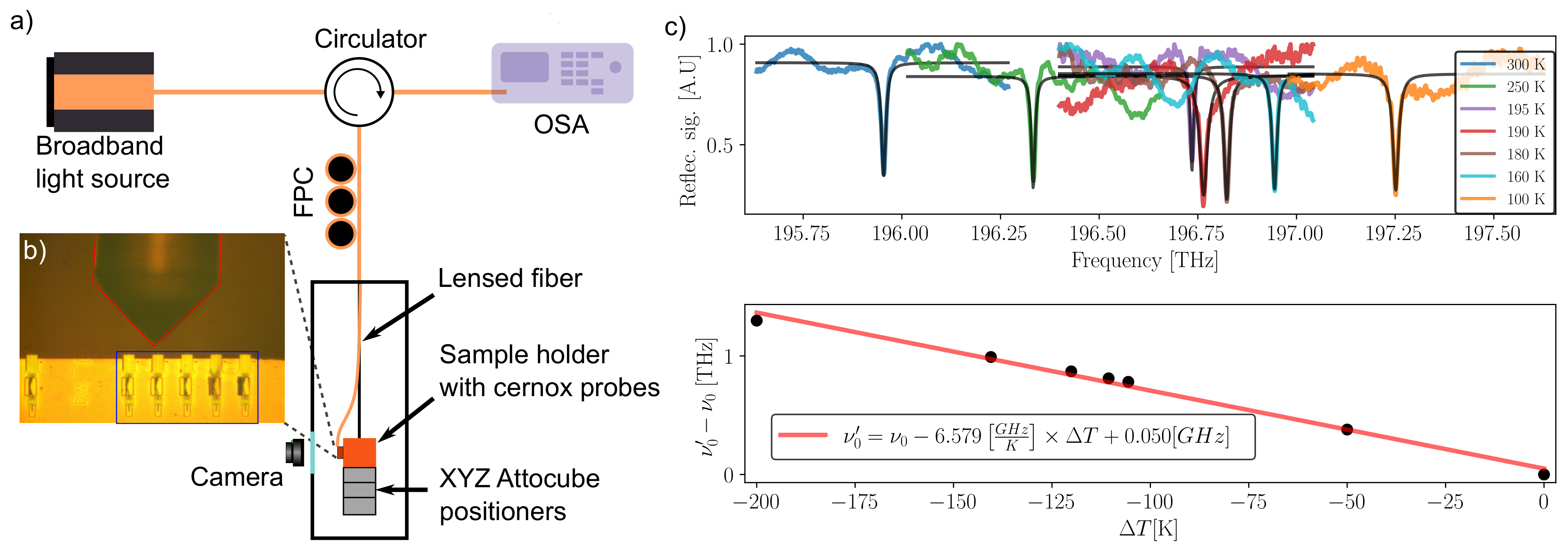
2.1. Concept and Instrumentation of Ring Resonator Based Photonic Thermometry

The basic concept of a photonic integrated circuit (PIC) is to guide and manipulate light in an optically transparent material. Especially in the near-infrared, silicon is one of the most frequently used materials for these PICs. For the manufacture of PIC with crystalline silicon of high material quality, silicon on insulator (silicon oxide, SiO 2 ) wafers are well established [6,7]. Using several clean room processes, the usually 220 nm thick silicon layer is structured and depending on the application could be covered with a cladding layer (SiO 2 , SiN, etc.) or it remains air cladded. The light guidance of the waveguide results from the refractive index contrast with the surrounding material. In our case, the silicon waveguides are cladded by a SiO 2 layer as the cross section in Figure 1 illustrates. Due to the sub-wavelength size of the light guiding structure, part of the energy is guided outside the waveguide. As a result, it is possible that a part of the light can evanescently couple to neighbouring waveguides like a circular shape ring resonator. This ring works as an optical cavity with a resonance at each wavelength λ m which fit m-times ( m N ) into the optical length of the waveguide [6,8]:
λ m = n eff ( T , λ ) L ( T ) m
with n eff as the effective refractive index, L is the length of ring waveguide and T the temperature. Due to thermal expansion and the thermo-optic effect, both L and n eff change with temperature [6,8]. For an ideal waveguide, Equation (1) leads to multiple narrow-band local minima in the transmittance. The quality factor Q describes the sharpness of the resonance as follows:
Q m = λ m FWHM m
where λ m is central wavelength of the resonance m and FWHM m the corresponding full width at half maximum. For temperature sensing applications, a large Q-factor allows a very precise detection of the peak wavelength due to the small FWHM . On the other hand, a high Q-factor together with high laser power leads to increased self-heating, which limits the temperature sensitivity [9,10]. The PICs used here are produced in production grade clean room facilities using the “SG25H5_EPIC” technology [7].
Figure 1 (lower part) shows the basic concept for the characterisation of PIC-based thermometers. The emission of a narrow-linewidth tuneable laser is split into a reference path for accurate wavelength determination and a measurement path that includes the PIC photonic thermometer. To manually adjust the optical power and polarisation, a variable attenuator and a polarisation controller are located in front of the PIC. The fibre-to-chip coupling is achieved by using two microstructured planar grating couplers. The transmitted spectrum passing through the PIC is guided to photoreceivers and digitized by analog-to-digital converter. For a reliable characterisation of the photonic structures, traceability of temperature and wavelength scales to the international system of units (SI) is important. More details on the set-up and its temperature stability and traceability can be found in Ref. [4]. Here, two options are used for in-situ determination of the wavelength (see Figure 1).
In option A, the laser light passes through a reference gas cell and is detected by a photoreceiver. Due to the known isotopic composition and pressure, the absorption spectrum of this standard reference material (SRM) is traceable to the SI according to [11]. To determine the absorption lines from the recorded spectrum, each peak is fitted by a Voigt function. The resulting differences between the tabulated peak positions of the gas absorption wavelengths and the measured absorption wavelengths in the gas cell transmission, as calculated internally by the laser, are used to compute a correction function that allows determination of the actual laser wavelength with a typical uncertainty of 0.6 pm [4]. Due to the MHz sampling rate of modern photoreceivers, this method enables SI traceability with fast wavelength tuning of up to 1000 nm/s. Consequently, an acquisition of a complete 100 nm spectrum (Figure 2a) with femtometer wavelength resolution takes less than 1 s.
Option B is based on a wavemeter, which uses a non-moving Fizeau interferometer to measure the laser wavelength with an accuracy of σ 0.08 pm. The SI traceability of this option is achieved by a regular calibration to a stabilized reference laser. To ensure this high wavelength resolution, the scanning speed must be relatively slow. With the typical wavemeter sampling rate of below 500 Hz, a monitoring of the laser wavelength with 0.2 pm resolution leads to 0.1 nm/s scanning speed. Consequently, the temporal stability of the temperature must be higher when using a wavemeter compared to the gas cells’ wavelength reference.
Comparing the two options shows that both have their specific use case. The gas cell offers a few advantages for the use of a PIC as an application-oriented temperature sensor. First of all, the gas cell is cost-effective (<$1000) and can be integrated in a portable housing together with the laser and the detector. Secondly, the high speed of the method is suitable for monitoring application. The wavemeter option offers a higher wavelength resolution and accuracy and needs a higher thermal stability, which fits to metrological applications with highly temperature stable calibration furnaces (e.g., fixpoint cells).
Using the thermostated platform, both options currently have comparable uncertainties. As an alternative to the described swept-wavelength mode where multiple resonances m (see Equation (1)) are measured, it is possible to lock the laser wavelength to a single resonance [2,12].

2.2. Characterization of the Optical and Thermal Response of the Photonic Thermometers

Figure 2 shows the data processing steps to determine the peak position λ m and FWHM m of the PIC. Figure 2a shows the transmittance spectrum of three ring resonators (see inset) with different radii (R1 …R3). The background signal (orange) results mainly from the transmission of the grating couplers, which are used for fibre-to-chip coupling. In the first step, this background is determined (two-step low-pass filtering) and the normalised transmittance of the resonators is determined by dividing the raw data by the background. In the next step (see Figure 2b), the local minima of the spectrum are determined. Subsequently, a Lorentz function is used to fit the data of each minima. The low amplitude residuals of the indiviudal fits (see Figure 2c) are a clear indicator that the resonances of the ring resonators can be described by a Lorentz function. Based on the fit parameter, the central wavelength λ m , the FWHM m and the extinction ratio are determined. We determined extinction ratios up to 21 dB with a mean FWHM between 10.4 pm and 13.3 pm and a mean Q-factor from 117,000 to 150,000.
Figure 3 (upper part) shows the resulting Q-factors for the three resonators at the temperatures 20 °C, 50 °C, and 80 °C. The small FWHM of roughly 10 pm corresponds to Q 150,000 and allows a peak detection with sub-pm resolution. A possible wavelength uncertainty of this peak position could be below 0.6 pm, as shown in [4]. The lower part of Figure 3 shows the individual extinction ratios. The results are summarized in Table 1. R2 shows the best mean Q-factor and extinction ratio compared to the other two ring resonators. Both performance parameters, Q and extinction ratio, show in our case no clear temperature dependence. However, we do see a decrease in Q-factor and extinction ratio with increasing wavelength, which could result from the change in n eff . We refer the reader to Bogaerts et al. [6] for further details on this topic.
Figure 4a shows the temperature sensitivity of R1, R2 and R3 silicon ring resonators. Changing the temperature from 20 °C to 80 °C systematically shifts the whole transmission spectrum of silicon ring resonators and the sharp resonance peak towards longer wavelengths with temperature sensitivity λ / T of 81 pm/°C (Figure 4a). Our results show residuals from linear and polynomial (4th degree) fittings of the silicon ring resonator sensitivity over the range of 20 °C to 80 °C (Figure 4b,c). Temperature sensitivity of the ring resonators shows reasonably good linear response with residuals below 0.1 nm; however, 4th degree polynomials have less than 0.02 nm residual with random distribution over the y = 0 horizontal line.

2.3. Effect of Optical Absorption on Thermal Equilibrium

The role of linear and nonlinear optical absorption plays a big part in the performance of optical resonators. Due to the strong confinement of the light to the optical cavity at resonance conditions, the build-up of photons in the resonator can reach immense numbers. This is further enhanced by the cavity optimization processes to reach high optical Q-factors. Generally, the studied materials have sufficiently high bandgap energies (Silicon: 1.13 eV [13], GaN: 3.4 eV [13], Diamond: 5.4 eV [14]) to be transparent for photons of wavelength λ = 1550 nm ( E phot = 0.79 eV). However, if the extreme intensities at resonance are taken into account, nonlinear absorption effects come into play. Two-Photon Absorption (TPA) arises when at high intensities two photons are absorbed simultaneously by a single electron, whereupon the electron is lifted to a higher state, reaching the conduction band and then is able to recombine, dissipating the excess energy as heat. This self-heating process leads to a distortion of the temperature measurement. An analytical model to describe this effect in microrings was developed (see Refs. [9,10]). TPA is more severe for materials with a smaller bandgap energy like silicon, where two simultaneously absorbed photons ( λ phot = 1550 nm) can easily lead to an electronic excitement for the conduction band ( E TPA = 2 E phot = 1.58 eV). The threshold intensity of the TPA-effect to dominate the absorption processes within the optical resonator was found to be I th = α mat / β mat , with α mat being the linear absorption coefficient and β mat the two-photon absorption coefficient of the respective material [9]. Hereby, a distinction has to be made between two cases: Firstly, the case of recombination of the electric carriers and the energy dissipation as heat leading to an increased device temperature, which ultimately red-shifts the resonance wavelength due to the thermo-optic effect. Secondly, the case of free carriers in the conduction band reducing the refractive index of the resonator material (Free Carrier Dispersion) and consequently leading to a blue-shift of the resonance wavelength [15]. These two cases can be distinguished as they come into play on different time scales [16]. The creation of free carriers due to TPA at sufficiently high intensities takes place within a few nano-seconds with a free-carrier lifetime of about t FC 10 ns, while the thermal recombination process requires more time (up to 100 ns) depending on the thermal conductance properties of the resonator design and material. To alleviate the self-heating effect, buried resonator designs could be considered in order to improve the thermal contact with the substrate (e.g., SiOx-cladding). Initial simulations have shown that self-heating due to optical absorption is even more critical in the nanobeam designs (SEM-image in Figure 5) compared with ring resonators.
This is likely due to the much smaller mode volume of the optical resonance in the nanobeam. As can be seen in Figure 6, even low input powers lead to considerable self-heating of the device and to operate the device with a self heating effect <1 mK, the power coupled to the resonator should be below 80 nW. The effect of TPA dominates at maximum intensities higher than I th = 10 12 Wm 2 (power coupled to the resonator >200 µW, see Figure 6).

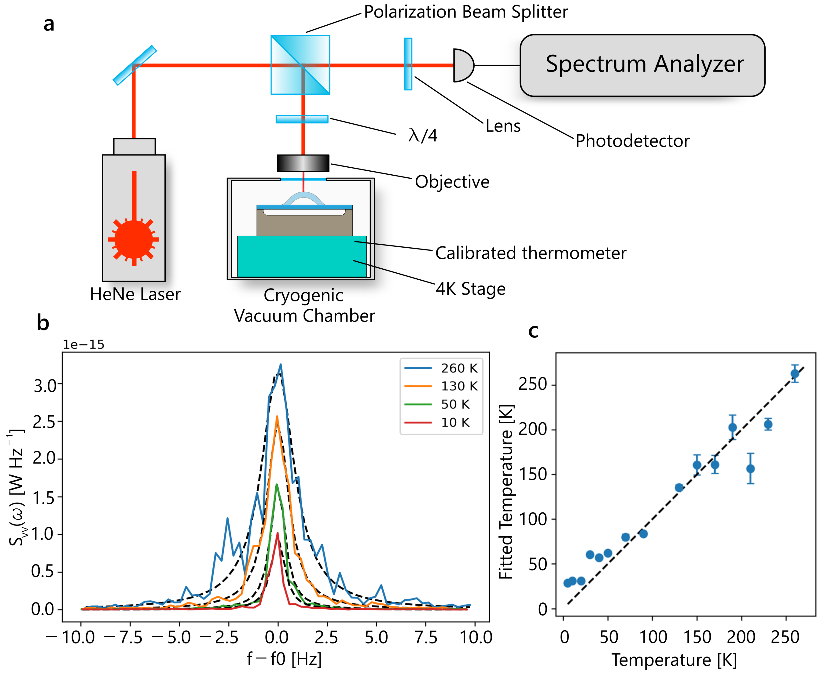
3. Optical Noise-Thermometry with Optomechanical Sensors

3.1. Measurement Principle and Measurement Equations

Thermomechanical noise is the noise caused by the Brownian thermal motion of particles at a given temperature, associated with an average kinetic energy per degree of freedom equal to E k = k B T / 2 . For optomechanical resonators, it results in mechanical excitations which generate microscopic fluctuations within the resonator itself related to its temperature. As a consequence, the resonator is thermally excited with a broadband random force with a power spectral density function S F F that is flat in frequency. At thermal equilibrium, the stationary thermal force noise S F F is related to the mechanical susceptibility χ ( ω ) by the fluctuation-dissipation theorem [17]:
S F F = 4 k B T ω Im 1 χ ( ω ) = 4 k B T m eff ω m Q m ,
where k B is the Boltzmann constant, T the temperature, m eff the effective mass of the mechanical mode, ω m the resonance frequency and Q m the quality factor. The susceptibility has a Lorentzian shape [17]:
χ ( ω ) = m eff ω m 2 ω 2 i ω ω m Q m 1
The one-sided power spectral density S x x ( ω ) of displacements experienced by the resonator can then be inferred from the mechanical susceptibility and the thermal force noise S F F [17]:
S x x ( ω ) = | χ ( ω ) | 2 S F F = 4 k B T ω m m eff Q m ω m 2 ω 2 2 + ω ω m Q m 2 .
Integrating S x x ( ω ) over all positive frequencies gives the variance of the mechanical displacement x 2 , which is equal to the area under the mechanical noise spectrum [18]:
x 2 = 1 2 π 0 S x x ( ω ) d ω = k B T ω m 2 m eff
Equation (6) shows that the thermodynamic temperature can be inferred from measurements of the area under the noise power produced by a optomechanical resonator of known effective mass (or stiffness), and might also be inferred from the peak in (5) using the measured Q and ω m . The temperature depends purely on the Boltzmann constant as long as the resonance frequency can be measured and the effective mass calculated. Therefore, the resonator can be used to develop a primary optical noise thermometer [19], which does not require independent calibration, similarly to a Johnson noise thermometer [5] and with the advantage that optical interrogation is immune to electrical noise and interference. If m eff or k eff = m eff ω m 2 are not exactly known, they might be determined using (6) from a measurement at a single known reference temperature. Once calibrated at this reference temperature, the optomechanical thermometer will provide an accurate temperature reading at all other temperatures based on (6), provided that its effective mass is independent of temperature.

3.2. Fabrication and Characterization of the Resonators

To experimentally validate the proposed thermometry scheme, we fabricated two types of optomechanical devices. The first ones are 2D square membranes (2DSM) with mechanical modes in the MHz domain, and the second are 1D suspended optomechanical crystals (1DOC) with mechanical modes in the GHz range.

3.2.1. Fabrication of Suspended 2D Square Membranes

The 2DSM are fabricated on high-stress silicon nitride, a material known for its ultra-low mechanical dissipation and hence high quality factor. Due to the high tensile stress, silicon nitride thin films can in fact exhibit quality factors as high as 10 6 [20]. Engineering the structure can then further reduce the losses and bring the quality factor over 10 8 [21,22,23].
A high quality factor for our optical noise thermometer is beneficial to increase the peak value of the power spectral density, which can be calculated from Equation (5):
S x x ( ω m ) = 4 k B T Q m ω m 3 m eff
This allows for detecting the small fluctuations of the resonator caused by thermomechanical noise, otherwise hidden by the noise floor.
At the same time, a high quality factor results in a small linewidth Γ m ( Q m = ω m / Γ m ) —typically down to a few mHz for silicon nitride resonators—which poses a challenge on the read-out protocol. In order to precisely extract the temperature from the mechanical displacement x 2 , the read-out protocol needs to measure the mechanical spectrum with sufficient data points around the peak, requiring a measurement bandwidth smaller than the resonator’s linewidth. To do so, one needs to acquire a long time trace and extract the mechanical properties from its Fourier transform, but this method exposes the measurement to artificial broadening mechanisms due to the shift of the resonance frequency during the measurement, limiting the minimum measurable linewidth. It follows that, for a reliable measurement of the temperature, the mechanical resonator needs to have a linewidth Γ m large enough to avoid shifting of the resonance frequency within the measurement time, while being small enough to have high enough Q and signal strength to detect the thermomechanical peak and precisely determine its resonance frequency.
To optimize this trade-off, we fabricated resonators with different devices and geometries which led to a wide range of quality factors up to 10 9 at room temperature [24]. Hence, we acquired the spectrum of each resonator and found that, above Q m = 10 7 , our read-out protocol cannot detect the change of the mechanical displacement x 2 as function of temperature, due to the low linewidth Γ m . All the measurements with 2DSM presented in this work are therefore performed on a square membrane of 80 nm thickness with an approximate quality factor Q m = 10 6 . As shown in Figure 7a, the membrane is patterned with holes of 450 nm radius and 1438 nm lattice constant, to allow the release of the structure from the silicon substrate underneath. Those holes affect the resonator’s mass-per-area reducing the effective mass, increasing the resonance frequency and keeping the effective stiffness k eff ( ω 2 m eff = k eff ) unchanged. The silicon nitride is deposited by low-pressure chemical vapor deposition on the silicon substrate. The pattern is first written by electron beam lithography into a resist and then transferred to the silicon nitride by a dry-etching step. Finally, the membrane is released with a dry etching step which isotropically etches the silicon substrate underneath. The fabricated membrane has an initial stress of 1.1 GPa, which leads to a resonance frequency of the fundamental flexural mode of 1.338 MHz for the square membrane with a side length of 250 μ m shown in Figure 7a.

3.2.2. Fabrication and Characterization of 1D Optomechanical Crystals

The optomechanical crystal is made of a 200 nm thick GaP membrane. Due to the strong refractive index ( n = 3.1 ) of this III-V semiconductor, light can be confined within this thin layer thanks to total internal reflection. Meanwhile, lateral confinement of light is performed by structuring the GaP layer into a 700 nm wide and approximately 20 μ m long waveguide. A ladder-like optical cavity is then performed by drilling holes with a diameter of 260 nm periodically positioned along the waveguide. Such a photonic structure is also called nanobeam cavity. At the center of the nanobeam cavity, the lattice constant ( a center = 410 nm) is chosen in order to allow a propagating mode at the targeted wavelength (around 1550 nm). From the center to the end of the nanobeam, periodicity is gradually increased till a position where the period is kept constant ( a end = 480 nm). It is chosen in order to have the targeted wavelength at the centre of the photonic band-gap. This method is known as gentle confinement and allows for reaching high optical quality factors. Here, for suspended nanobeam cavities, we achieve a simulated optical quality factor of 10 7 . Beyond the confinement of photons, such structures also display evidence of phononic confinement in the GHz frequency range. With the designed crystal, the fundamental mechanical modes are co-localized with their optical counterparts, and are resonating at 2.5 GHz. Nowadays, such crystals confining at the same time photons and phonons are named optomechanical crystals. The coupling between photonic and phononic degrees of freedom can be simulated via finite element modeling, taking into account the two major contributions based on moving boundaries and photo-elastic effects. With the designed structures, the expected optomechanical coupling ( g 0 / 2 π ) is equal to 50 kHz. Fabrication of such devices has been performed using standard nanofabrication techniques.
Optical characterization of the 1DOC has been performed with the fiber setup shown in Figure 8a. The sample is inserted into a circulating liquid Helium cryostat at a low pressure (few mBar) of helium exchange gas. The copper sample holder is equipped with Cernox sensors both in the bulk and on the surface to identify potential temperature gradients. The white light of a superluminescent light emitting diode (SLED) is injected and collected back with a lensed fiber and analyzed with an OSA. The alignment is performed with a 3-stage attocube micropositioners and monitored from the outside of the cryostat with a camera mounted on a microscope, as one can see in Figure 8b. A polarization controller (FPC) is used to tune the polarization of the light before it reaches the sample. This component has to be carefully adjusted to align the linear polarization to the on-chip waveguide and to minimize optical losses when the reflected light goes through the OSA via the circulator. Due to birefringence in fibers, this cannot be achieved for every wavelength and wiggles on top of the reflection curves presented in Figure 8 show a slight dependence of the polarization with the frequency of light. This effect is nevertheless not detrimental to the measurement as optical resonance presents a clear dip in the reflection due to absorption of the resonant light in the photonics crystal or transmission through it to the bulk.
The studied resonators exhibit optical modes in the telecom wavelength range λ 0 1550 nm, with optical Q-factors of the order of 10 5 . The optical resonance frequency of the optical resonator depends on the effective temperature of the crystal. This effect can be explained by the modification of the refractive index of the material with temperature ( Δ n / Δ T / n 3 × 10 5 K 1 for GaP) and, at a lower level, by the thermal expansion of the structure ( α < 4 × 10 6 K 1 for GaP). Figure 8c demonstrates this behaviour: the top figure shows the evolution of the optical resonance frequency ν 0 , monitored with the setup displayed in Figure 8a, while changing the cryostat’s temperature from 300 K to 100 K. Each curve has been fitted with a Lorentzian line shape, from which ν 0 was extracted and plotted against the temperature variation Δ T . A linear fit of these data allows one to extract from its slope the shift coefficient β ( ν 0 ) that includes both the contributions of the thermo-refractive effect and the thermal expansion to the ν 0 , we find β ( ν 0 ) = −6.58 GHz K 1 in a good agreement with [25]. This frequency shift is used further in Section 3.4 to study the thermal contribution of the probe laser.

3.3. Thermometry Measurements

3.3.1. Thermometry with Suspended Square Membranes

Figure 9b shows the measured power spectra S V V ( ω ) on the photodiode that is proportional to S x x ( ω ) , acquired at four different temperatures from 260 K to 10 K by a spectrum analyzer with the measurement setup in Figure 9a. The mechanical displacement is probed using a Helium Neon (HeNe) laser (632.8 nm) and the mechanical resonator is mounted inside a cryogenic vacuum chamber, at a pressure of the order of 10 6 mbar. The sample holder is equipped with a ITS-90 calibrated commercial thin film resistance temperature sensor, which assures IT-90 traceability. The linearly polarised laser beam from the HeNe laser is sent first through a polarization beam splitter, transparent for vertically polarized light, and then through a λ 4 plate rotated at 45 , circularly polarizing the light. The light is then focused on the sample by a ×20 objective. The focused light is partially reflected by the suspended silicon nitride membrane, partially transmitted to the underneath silicon substrate and reflected by it, creating a Fabry–Perot cavity. The interference between the different light paths results in a position dependent light intensity that is used to determine the membrane’s motion. The reflected light passes again through the λ 4 plate and is focused on the photodiode, connected to a spectrum analyzer which allows for extracting the Brownian motion [26].
As expected from Equations (5) and (6), the measured power spectra S V V ( ω ) and mechanical displacement x 2 exhibit a clear dependence on the temperature of the resonator. To determine S x x ( ω ) , the data are first pre-processed with a binning algorithm to reduce the noise. Then, a thermomechanical calibration of the measurement setup [17] is performed using the spectrum acquired at a temperature T=260 K determined using the Cernox sensor. This last step allows for obtaining the conversion factor from S V V ( ω ) to S x x ( ω ) . After that, the spectrum acquired at each temperature can be fitted by Equation (5), where m eff is analytically calculated using the reference measurement at T=260K and the values of Q m and ω m obtained from the fits. Finally, the temperature of the resonator is calculated by integrating the fitted curve S x x ( ω ) and obtaining the mechanical displacement x 2 . At each temperature, the focus on the sample is adjusted to ensure a comparable sensitivity over the entire temperature range. We note that this procedure can introduce additional uncertainty in the conversion factor, which should be eliminated in the final implementation of the thermometry protocol, e.g., using a calibration tone as described for the 1DOC devices below. Figure 9c shows the fitted temperature for each measurement, compared to the temperature of the resonator obtained from the independent calibrated commercial sensor. The error bars indicate the standard deviation for each measurement. Measurements with a standard deviation larger than 20 K are discarded. This result shows reasonable agreement between the optical noise-thermometry method and the temperature obtained from the independent calibrated sensor over the range of 5 K to 260 K, providing evidence for the potential of the described thermometry technique. Due to the small linewidth and peak-height at low temperatures, the error bars and uncertainty in the optomechanical noise-thermometry increase at low temperatures, causing deviations from the temperature obtained from the independent calibrated sensors. The positive deviation of the temperature at low might partly be attributed to a systematic overestimation of the peak area by the employed fitting routine.

3.3.2. Thermometry with Optomechanical Crystals

Noise-thermometry measurements with 1DOC are done with the fiber setup depicted in Figure 10a by partially reusing the setup described in Section 3.2.2. The light source is a telecom tunable laser whose frequency is set at the edge of the optical mode’s resonance near the half of the peak depth for a maximum detection sensitivity. The displacements of the resonator are then directly transduced into an intensity modulation of the reflected light. The reflected beam is finally amplified with an erbium-doped fiber amplifier (EDFA) before detection with a high-speed photodiode. The resulting photocurrent is split into DC (optical resonance monitoring) and RF signals. The latter is amplified with low-noise RF amplifiers before reading-out the signal with an ESA.
Due to thermal expansion of the sample holder, one has to realign the sample with respect to the fiber at each temperature. Moreover, the optical frequency shifts with temperature and the side of fringe measurement scheme implies that, from one temperature to another, the sensitivity is potentially not the same. In order to calibrate the power noise in terms of displacement noise density, a phase modulation is applied on the beam with an EOM at a frequency Ω mod within a few Megahertz of the mechanical resonance frequency ω m . Having Ω mod in the vicinity of ω m allows for assuming that the displacement-to-voltage transduction factor of both the calibration tone and Brownian motion are nearly the same. The calibration phase modulation δ φ gives a reference of displacement transduction in the optomechanical crystal regardless of optical alignment, optical detuning and amplification chain, as it is equivalent to a displacement δ x according to:
δ x L = Ω mod δ φ ν 0 ,
where L is the optical length of the cavity and ν 0 the frequency of the laser.
Measured spectra are fitted by Lorentzian lineshapes for the Brownian motion, and with Gaussian lineshapes for the calibration peaks (black lines in plots on the left panel of Figure 10b). The Brownian motion peak is then renormalized by dividing its area by the one of the calibration peak, yielding a ratio R T , which, according to (6), is proportional to temperature R T T mode , where T is the set temperature and T mode is the fundamental mechanical mode’s temperature. Assuming a good thermalization of the fundamental mode at T cryo = 296 K , meaning that T cryo = T mode . R T is set as a reference and the subsequent temperature are computed as follows:
T noise = 296 K × R T R 296 K
The resulting temperatures are plotted against the temperature measured by the Cernox temperature sensor, as one can see in the right panel of Figure 10b. The data points are fitted with a linear function. With the exception of the second data point at 180 K, the inferred temperatures are within the fit error. This discrepancy might be explained by a hybridization with a nearby second mechanical modes, as can be seen in the corresponding noise spectrum in Figure 10b that affects the convergence of the fit and the extracted value of R T . Further analysis is required to confirm this hypothesis.

3.4. Investigation of Systematic Errors

Let us now investigate the effect of systematic errors on the temperature measurement precision and accuracy. We focus mainly on the effect of optical heat absorption on the measured temperatures.

3.4.1. Effect of Optical Absorption on Suspended Membranes

Employing a high laser power is beneficial for increasing the resonance signal level well above the measurement noise floor. However, high laser power can lead to photothermal effects due to absorption of laser light, leading to an incorrect measurement of the temperature. To study this effect, we acquired thermomechanical noise spectra at a constant temperature of T = 5 K for different values of the laser power (Figure 11b), with the mechanical characterization setup depicted in Figure 9 and used a finite-element model of our resonator to numerically analyse the absorbed optical power and the resulting temperature distribution using Comsol. The material parameters are Young’s modulus E = 270 GPa, mass density ρ = 3200 kg/m 3 , and Poisson’s ratio ν = 0.27 , while the assumed optical properties are thermal conductivity k = 20 W(mK) 1 , thermal expansion coefficient α = 2.3 × 10 6 K−1 and heat capacity C p = 700 J kg 1 K 1 ) [27]. The laser heating is simulated assuming a Gaussian beam profile at the center of the resonator and the outer boundaries of the resonator are set to 5 K. The result in Figure 11a shows a localized temperature increase in the center of the 2DSM of 0.18 K at an incident laser power of 64.39 μ W, the highest value employed in the measurement. The laser power absorbed by the SiN membrane is 0.64 μ W, 1.01% of the incident power [28]. The localized laser heating, and associated temperature increase, has a three-fold effect on the developed noise-thermometry scheme: the resonance frequency decreases as a result of the tension induced by thermal expansion, the area under the S x x spectrum increases according to (5) and the signal on the photodiode increases due to the larger conversion factor at higher laser power. Figure 11c shows the change in resonance frequency as a function of incident laser power, where a linear relation can be observed as expected. From this relation, the average temperature change in the SiN membrane can be estimated using literature values of the thermal expansion coefficient α = 2.3 × 10 6 K−1 and Young’s modulus E = 270 GPa, using Δ f = α E Δ T f 0 / n pre , using the prestress of n pre = 1.1 GPa in the membrane and its resonance frequency f 0 = 1.33 MHz. With this estimation formula, the frequency shift of Δ f = 60 Hz in Figure 11c is estimated to correspond to an average temperature increase Δ T = 80 mK, a value that is of the same order of magnitude as the simulated temperature increases in Figure 11a. This calculation also shows that the resonance frequency can be an accurate measure of temperature that might complement noise thermometry protocols for reaching higher precision temperature measurements, while using thermomechanical noise for accuracy and self-calibration. In Figure 11d, the temperature at every laser power was determined using noise thermometry, by integrating the fitted area under the peaks in Figure 11b with Equation (6). Prior to the fits shown in Figure 11b, an additional thermomechanical calibration step is performed for all the spectra, providing for each laser power a conversion factor from S V V ( ω ) to S x x ( ω ) . However, the error in the temperature measurement using this procedure is larger than the laser-induced temperature changes of 80 mK, such that the effect of laser power on temperature cannot be as clearly resolved as by using the resonance frequency shift in Figure 11c.

3.4.2. Effect of Optical Absorption in Optomechanical Crystals

In the following, we estimate the thermal contribution of the probe’s optical power absorption on the 1DOC. This estimate relies on an optomechanical static nonlinear effect equivalent to a Kerr effect where the refractive index of the material depends on the optical power. This leads to a deformation of the optical resonance when scanning the laser wavelength and even could end up in an optical bistability. In our case, this phenomenon is likely induced by the absorption of light circulating inside the optical cavity that causes a temperature increase of the optomechanical crystal and changes in the refractive index. This behaviour is presented in Figure 12a where, at medium input power, the optical resonance leaves the Lorentzian shape and shows a more and more triangular shape where the resonance frequency is shifted toward low frequency. At high input power, the resonance even exhibits a bistable behaviour with a rapid drop just after reaching the resonance frequency. All curves in Figure 12a are obtained by sweeping the laser from high to low frequency. When sweeping the laser frequency up, hysteresis can be observed for the curves obtained at 100 and 200 μ W.
The minima of each curve of Figure 12a have been extracted and plotted against the input power P i n t . A linear fit of the data points gives a shift coefficient equal to α rad = −0.166 GHz/ μ W. The temperature variation Δ T is then estimated by combining this frequency shift and the shift coefficient obtained in Figure 8c. The resulting heating induced by optical absorption is depicted in Figure 12b with Δ T = α r a d × P + 4.25 α t h 0.05 K.

4. Conclusions

The measurement of temperature using photonic on-chip thermometers is of growing interest to the scientific and industrial communities. This interest is driven by the potential to perform thermometry in harsh environments, with sensors that provide accurate readings while providing advantages in terms of linearity and calibration. In this article, we provide experimental studies on a variety of photonic and optomechanical thermometers demonstrating different sensing and calibration approaches. With the photonic devices, a very high temperature sensitivity of 81 pm/K is demonstrated, while accuracy is enhanced using a gas cell to determine the laser wavelength. Photomechanical noise-thermometry on nanomechanical devices was applied to measure temperatures over the range from 5 K to 300 K. Due to the linearity provided by the equipartition theorem, a single calibration was sufficient to determine temperature over the whole temperature range. Limitations in terms of optothermal self-heating of the sensors were assessed to provide optimal operation conditions. The resolution of the temperature measurement (error bars in Figure 9c) is limited by experimental factors like stability, self-heating and the accuracy by which the thermomechanical noise peak can be characterized. In future studies and applications, the presented technologies might be merged on a single chip, to combine the high-precision of photonic thermometry with the self-calibration potential of optomechanical thermometers.

Author Contributions

Experiments, methodology and investigation, T.B., S.K. (Stephan Krenek), A.C. (Andrea Cupertino), R.A.N., F.L., R.E., S.K. (Stefanie Kroker), W.D., S.T., O.H., S.P., O.K., M.J.M., L.Z., G.W., T.M., L.W. and D.R.; data analysis, F.L., R.E., S.K. (Stephan Krenek), D.S., S.T., O.H., S.P., S.K. (Stefanie Kroker), W.D. and A.C. (Andrea Cupertino); writing, T.B., S.K. (Stephan Krenek), R.E., A.C. (Andrea Cupertino), F.L., R.B., L.W., A.C. (Alberto Casas), P.G.S. and S.B.; supervision, P.A.P., D.R., S.K. (Stefanie Kroker), S.K. (Stephan Krenek), R.A.N., P.G.S. and S.B.; project administration and funding acquisition, S.B. All authors have read and agreed to the published version of the manuscript.

Funding

This work was carried out under the 17FUN05 PhotOQuanT project, which has received funding from the EMPIR program, co-financed by the Participating States and the European Union’s Horizon 2020 research and innovation program.

Institutional Review Board Statement

Not applicable.

Informed Consent Statement

Not applicable.

Data Availability Statement

Derived data supporting the findings of this study are available on request.

Acknowledgments

A.Cupertino, P.G.S. and R.N. acknowledge valuable support from Herre van der Zant. A.Cupertino, P.G.S. and R.N. would also like to thank Makars Šiškins, Gabriele Baglioni and Maurits Houmes for stimulating discussions and assistance with experiments.

Conflicts of Interest

The authors declare no conflict of interest.

References

  1. Fellmuth, B.; Fischer, J.; Machin, G.; Picard, S.; Steur, P.P.M.; Tamura, O.; White, D.R.; Yoon, H. The kelvin redefinition and its mise en pratique. Phil. Trans. R. Soc. A 2016, 374. [Google Scholar] [CrossRef] [PubMed]
  2. Klimov, N.; Purdy, T.; Ahmed, Z. Towards replacing resistance thermometry with photonic thermometry. Sens. Actuators A Phys. 2018, 269, 308–312. [Google Scholar] [CrossRef] [PubMed]
  3. Purdy, T.P.; Grutter, K.E.; Srinivasan, K.; Taylor, J.M. Quantum correlations from a room-temperature optomechanical cavity. Science 2017, 356, 1265–1268. [Google Scholar] [CrossRef] [PubMed] [Green Version]
  4. Eisermann, R.; Krenek, S.; Winzer, G.; Rudtsch, S. Photonic contact thermometry using silicon ring resonators and tuneable laser-based spectroscopy. Tech. Mess. 2021, 88, 640–654. [Google Scholar] [CrossRef]
  5. Qu, J.F.; Benz, S.P.; Rogalla, H.; Tew, W.L.; White, D.R.; Zhou, K.L. Johnson noise thermometry. Meas. Sci. Technol. 2019, 30, 112001. [Google Scholar] [CrossRef]
  6. Bogaerts, W.; De Heyn, P.; Van Vaerenbergh, T.; De Vos, K.; Kumar Selvaraja, S.; Claes, T.; Dumon, P.; Bienstman, P.; Van Thourhout, D.; Baets, R. Silicon microring resonators. Laser Photonics Rev. 2012, 6, 47–73. [Google Scholar] [CrossRef]
  7. Zimmermann, L.; Knoll, D.; Kroh, M.; Lischke, S.; Petousi, D.; Winzer, G.; Yamamoto, Y. BiCMOS Silicon Photonics Platform. In Proceedings of the Optical Fiber Communication Conference. Optical Society of America, Los Angeles, CA, USA, 22–26 March 2015; p. Th4E.5. [Google Scholar] [CrossRef]
  8. Rabus, D.G. Ring resonators: Theory and modeling. In Integrated Ring Resonators: The Compendium; Springer: Cham, Switzerland, 2007; pp. 3–40. [Google Scholar]
  9. Weituschat, L.M.; Dickmann, W.; Guimbao, J.; Ramos, D.; Kroker, S.; Postigo, P.A. Photonic and thermal modelling of microrings in silicon, diamond and gan for temperature sensing. Nanomaterials 2020, 10, 934. [Google Scholar] [CrossRef]
  10. Dickmann, W.; Weituschat, L.M.; Eisermann, R.; Krenek, S.; Postigo, P.A.; Kroker, S. Heat dynamics in optical ring resonators. Model. Asp. Opt. Metrol. VIII 2021, 11783, 1178309. [Google Scholar]
  11. Gilbert, S.L.; Swann, W.C.; Wang, C.M. Hydrogen cyanide H13C14N absorption reference for 1530 nm to 1565 nm wavelength calibration–SRM 2519a. NIST Spec. Publ. 2005, 260, 137. [Google Scholar]
  12. Xu, H.; Hafezi, M.; Fan, J.; Taylor, J.M.; Strouse, G.F.; Ahmed, Z. Ultra-sensitive chip-based photonic temperature sensor using ring resonator structures. Optics Express 2014, 22, 3098–3104. [Google Scholar] [CrossRef]
  13. Streetman, B.G.; Banerjee, S. Solid State Electronic Devices, 7th ed.; Pearson Education: Harlow, UK, 2015; p. 580. [Google Scholar]
  14. Kittel, C. Introduction to Solid State Physics, 8th ed.; Wiley: Hoboken, NJ, USA, 2004; p. 190. [Google Scholar] [CrossRef]
  15. Almeida, V.R.; Barrios, C.A.; Panepucci, R.R.; Lipson, M. All-optical control of light on a silicon chip. Nature 2004, 431, 1081–1084. [Google Scholar] [CrossRef] [PubMed]
  16. Johnson, T.J.; Borselli, M.; Painter, O. Self-induced optical modulation of the transmission through a high-Q silicon microdisk resonator. Opt. Express 2006, 14, 817–831. [Google Scholar] [CrossRef] [PubMed]
  17. Hauer, B.; Doolin, C.; Beach, K.; Davis, J. A general procedure for thermomechanical calibration of nano/micro-mechanical resonators. Ann. Phys. 2013, 339, 181–207. [Google Scholar] [CrossRef] [Green Version]
  18. Aspelmeyer, M.; Kippenberg, T.J.; Marquardt, F. Cavity optomechanics. Rev. Mod. Phys. 2014, 86, 1391–1452. [Google Scholar] [CrossRef]
  19. Steeneken, P.G.; Le Phan, K.; Goossens, M.J.; Koops, G.E.J.; Brom, G.J.A.M.; van der Avoort, C.; van Beek, J.T.M. Piezoresistive heat engine and refrigerator. Nat. Phys. 2011, 7, 354–359. [Google Scholar] [CrossRef]
  20. Verbridge, S.S.; Parpia, J.M.; Reichenbach, R.B.; Bellan, L.M.; Craighead, H.G. High quality factor resonance at room temperature with nanostrings under high tensile stress. J. Appl. Phys. 2006, 99, 124304. [Google Scholar] [CrossRef] [Green Version]
  21. Norte, R.A.; Moura, J.P.; Gröblacher, S. Mechanical Resonators for Quantum Optomechanics Experiments at Room Temperature. Phys. Rev. Lett. 2016, 116, 147202. [Google Scholar] [CrossRef]
  22. Tsaturyan, Y.; Barg, A.; Polzik, E.S.; Schliesser, A. Ultracoherent nanomechanical resonators via soft clamping and dissipation dilution. Nat. Nanotechnol. 2017, 12, 776–783. [Google Scholar] [CrossRef]
  23. Ghadimi, A.H.; Fedorov, S.A.; Engelsen, N.J.; Bereyhi, M.J.; Schilling, R.; Wilson, D.J.; Kippenberg, T.J. Elastic strain engineering for ultralow mechanical dissipation. Science 2018, 360, 764–768. [Google Scholar] [CrossRef] [Green Version]
  24. Shin, D.; Cupertino, A.; de Jong, M.H.J.; Steeneken, P.G.; Bessa, M.A.; Norte, R.A. Spiderweb Nanomechanical Resonators via Bayesian Optimization: Inspired by Nature and Guided by Machine Learning. Adv. Mater. 2022, 34, 2106248. [Google Scholar] [CrossRef]
  25. Schneider, K.; Baumgartner, Y.; Hönl, S.; Welter, P.; Hahn, H.; Wilson, D.J.; Czornomaz, L.; Seidler, P. Optomechanics with one-dimensional gallium phosphide photonic crystal cavities. Optica 2019, 6, 577–584. [Google Scholar] [CrossRef]
  26. Davidovikj, D.; Slim, J.J.; Cartamil-Bueno, S.J.; van der Zant, H.S.J.; Steeneken, P.G.; Venstra, W.J. Visualizing the Motion of Graphene Nanodrums. Nano Lett. 2016, 16, 2768–2773. [Google Scholar] [CrossRef] [PubMed]
  27. Sadeghi, P.; Tanzer, M.; Luhmann, N.; Piller, M.; Chien, M.H.; Schmid, S. Thermal Transport and Frequency Response of Localized Modes on Low-Stress Nanomechanical Silicon Nitride Drums Featuring a Phononic-Band-Gap Structure. Phys. Rev. Appl. 2020, 14, 024068. [Google Scholar] [CrossRef]
  28. Chien, M.H.; Brameshuber, M.; Rossboth, B.K.; Schütz, G.J.; Schmid, S. Single-molecule optical absorption imaging by nanomechanical photothermal sensing. Proc. Natl. Acad. Sci. USA 2018, 115, 11150–11155. [Google Scholar] [CrossRef] [PubMed] [Green Version]
Figure 1. (Upper part): The basic concept of photonic thermometry based on photonic integrated circuits (PICs) is the determination of the temperature dependent resonance wavelength shift. (Lower part): Sketch of the set-ups used for the precise thermal and optical characterisation of PICs with two different options for the traceability of the wavelength to the international system of units.
Optics 03 00017 g001
Figure 2. Data Processing of the photonic integrated circuit spectra with three ring resonators (inset). (a) Raw data of PIC transmittance and estimated background, arising from grating coupler and optical setup; (b) The PIC transmittance, normalised by the background, shows the characteristics of the resonators. A Lorentz fit of the peak region is used to determine the exact position of λ m and other parameters. (c) Residuals of the peak fits.
Optics 03 00017 g002
Figure 3. Q-factor (a) and extinction ratio (b) of the three ring resonators between 1530 nm to 1570 nm for different temperatures of the thermostated platform.
Optics 03 00017 g003
Figure 4. (a) Sensitivity of three different silicon ring resonators with radius of R 1 = 35.048 µm, R 2 = 35.149 µm and R 3 = 35.037 µm and gap of 470 nm, 485 nm and 500 nm between the waveguide and resonator, respectively. Residuals of (b) linear fit, and (c) 4th degree Polynomial fit.
Optics 03 00017 g004
Figure 5. (a) SEM image of the fabricated photonic crystal nanobeam; (b) close-up of the nanobeam including measurement of the coupling gap (A), waveguide width (B), and hole diameters (C–E) of the photonic cavity (units are in nanometers).
Optics 03 00017 g005
Figure 6. Simulation of the self-heating of the nanobeam design (Silicon) versus the maximum intensity and power within the optical cavity. Below the threshold intensity I th = α / β , linear absorption dominates the self-heating effect, while at higher intensities the nonlinear two-photon absorption becomes more relevant.
Optics 03 00017 g006
Figure 7. (a) Optical microscope image of the suspended square membrane. The blue color is from thin-film interference effects of the not suspended silicon nitride on silicon substrate. (b) Electronic microscope image of the suspended GaP OMC, in yellow, the inverse taper waveguide, clamping point in light green and the cavity in red. (Colors are artificial).
Optics 03 00017 g007
Figure 8. Optical setup and photonic results. (a) Schematic of the photonic characterization setup. A broadband light source (SLED) is used to align the sample with respect to the fiber using XYZ attocube micropositioners. The reflected signal is monitored with an optical spectrum analyzer (OSA). FPC: Fibered polarization controller; (b) image from the alignment camera, the fiber is outlined in red and the samples in blue; (c) optical resonance frequency shift due to thermorefractive and thermal expansion effects.
Optics 03 00017 g008
Figure 9. (a) Schematic of the mechanical characterization setup. The mechanical resonator is placed inside a cryogenic vacuum chamber and the displacement caused by Brownian motion. Interference between reflected laser light reflected from substrate and membrane causes a displacement dependent intensity on a photodiode that is detected using a spectrum analyzer; (b) thermomechanical noise spectra at different temperatures obtained using a spectrum analyzer. The x-axis is centered at the fundamental resonance frequency f 0 of each spectrum for comparison. Dashed lines represent fits using (5). (c) temperature extracted from the measurements in (a) by integrating the area under the peak. The error bars show the standard deviation.
Optics 03 00017 g009
Figure 10. (a) Schematic of the calibrated noise-thermometry measurement setup. The optomechanical crystal is placed in a 4 He cryostat. The acquisition of the Brownian motion spectra, via the electrical spectrum analyzer (ESA), relies on the side of fringe measurement scheme. EOM: Electro-optical phase modulator; EDFA: Erbium-Doped Fiber Amplifier; PD: High-speed photodiode; (b) Left: Brownian motion spectra with their calibration tone at different temperatures. Right: Extracted temperature from the ratio of the areas of the Brownian motion and calibration peaks. The red curve is a linear fit to the extracted data.
Optics 03 00017 g010
Figure 11. (a) Simulated temperature distribution plot with an incident power P = 64.39 μ W; (b) thermomechanical noise spectra measured at a temperature of 5 K for different laser powers. The x-axis is the difference in frequency from the resonance frequency measured with a laser power of 64.39 μ W, equal to 1.331 MHz. (c) measured resonance frequency difference versus laser power with respect to the resonance frequency acquired with a laser power of 64.39 μ W; (d) temperature extracted from the measurements in (b) by integrating the area under the peak versus laser power.
Optics 03 00017 g011
Figure 12. Bistability of the optical resonance frequency with increasing input power. (a) Evolution of the Lorentzian optical mode into a bistable one with increasing power. (b) The local minima of each curve of Figure 12a are plotted against the input power and linearly fitted to extract the shift coefficient.
Optics 03 00017 g012
Table 1. Summary of the determined characteristics of the 126 resonances of each resonator in the wavelength range from 1530 nm to 1560 nm. For the Q-factor and FWHM , the mean value and its standard deviation are given for the individual resonators.
R1R2R3
Radius/µm35.04835.14935.037
FSR /nm (@ 1550 nm)2.8362.8272.836
Q-factor / 10 5 1.17 ± 0.081.50 ± 0.081.24 ± 0.07
FWHM /pm13.3 ± 0.910.4 ± 0.612.5 ± 0.8
Extinction ratio/dB6 …128 …218 …20
Sensitivity/pm/K81.1881.1581.15
Publisher’s Note: MDPI stays neutral with regard to jurisdictional claims in published maps and institutional affiliations.

