Investigation of Ocean Sub-Surface Processes in Tropical Cyclone Phailin Using a Coupled Modeling Framework: Sensitivity to Ocean Conditions

Abstract

The present study is aimed to investigate sub-surface ocean processes and their contribution to the intensification of a tropical cyclone (TC) from a coupled-modeling perspective. The Coupled Ocean–Atmosphere–Wave–Sediment Transport (COAWST) model was employed to simulate TC Phailin, which originated over the Bay of Bengal and made landfall on the eastern coast of India in October 2013. Three sub-surface ocean condition datasets—viz., (a) the European Centre for Medium-Range Weather Forecast (ECMWF) Ocean Reanalysis, (b) the Climate Forecast System Version 2 (CFSV2) Operational Analysis, and (c) the Hybrid Coordinate Ocean Model (HYCOM) Reanalysis datasets—were used for the initial and boundary conditions for the oceanic component of the coupled model in three different simulations of TC Phailin. All the simulations showed a delay in intensification compared to the observation, and ECMWF simulated the most intensified TC. CFSV2 simulated a deeper mixed layer (ML) and higher mixing, which hindered the intensification. Furthermore, higher entrainment of cold water in the ML led to cold water reaching the surface and, consequently, decreased sea surface temperature, which acted as negative feedback in the intensification of the storm in the cases of CFSV2 and HYCOM. ECMWF realistically simulated the interactions of the TC with a cold-core eddy before landfall. A sudden increase in ML heat content, the addition of heat in the ML due to entrainment, and the prevention of cold water reaching the surface were indicative of the breaking of the barrier layer (BL) in ECMWF, which was further corroborated by the spatial distribution of BL thickness in the simulation. This acted as positive feedback in the intensification of the TC. The findings of this study strongly suggest that not only the incorporation of physical oceanic sub-surface processes in the modeling of TCs but also the proper representation of prevailing mesoscale features and ocean sub-surface temperature, salinity, and current profiles in datasets is essential for realistic simulations of TCs.

1. Introduction

The densely populated eastern coastal states of India, especially the states of Odisha, Andhra Pradesh, and West Bengal, are prone to the landfall of severe tropical cyclones (TCs) originating in the Bay of Bengal (BoB) in the pre-monsoon (April–May) and post-monsoon (September–November) seasons. Landfall of TCs leads to catastrophic damage associated with the destruction of infrastructure and communication systems, coastal inundation caused by huge storm surges, and, lastly, loss of lives. It has been reported that almost 5% of global TCs form over the BoB [1]. The India Meteorological Department (IMD) recorded two of the deadliest cyclones in the BoB in the years 1977 and 1999. The TC that made landfall at Diviseema, Andhra Pradesh, in 1977 generated winds exceeding 250 km·h⁻¹. The Super Cyclonic Storm that hit the Odisha coast in 1999 resulted in 10,000 casualties and caused such extensive damage that the state of Odisha was left paralyzed for a long time. On 12 October 2013, the Very Severe Cyclonic Storm Phailin made landfall on the Odisha coast, south of Brahmapur, and, due to its severity, it brought back memories of 1999. TC Phailin, the second most intense post-monsoon TC over the BoB, wreaked havoc in the states of Odisha and, adjoining it to the north, Andhra Pradesh and claimed 45 lives in the process. Despite a massive improvement in forecasting and early warning systems, the destruction of infrastructure and property worth hundreds of millions of dollars could not be avoided. The accurate forecasting of the intensity and track of TCs is still a challenge for the scientific community, and one of the major factors that contribute to the uncertainty in forecasting TC intensity is the lack of understanding of sub-surface ocean processes, especially in the upper layers, and their interactions with the atmosphere during the occurrence of a TC [2,3]. Unfortunately, a very limited number of studies have been carried out to understand this aspect in the context of the BoB basin.

The ocean acts as the biggest source of energy for TCs by means of evaporation [4]. Hence, the SST plays a crucial role in the formation, maintenance, and intensification of TCs [2,5,6]. A study found the maximum attainable intensity of a TC to be a function of the SST [7]. Another study on the Odisha Super Cyclone (1999) using the Fifth-Generation Community Mesoscale Model (MM5) suggested that the storm intensity and track are greatly impacted by the SST field and its resolution [8]. In other studies, it was shown that the incorporation of high-resolution SSTs considerably impacts simulations of TCs using numerical models as it changes the diabatic heating structure near the core of the TCs [9,10]. A study on typhoon Maemi (2003) inferred that the movement of the storm, induced by different SSTs, was larger in the east–west direction than in the north–south direction [11]. BoB is a semi-enclosed basin in the North Indian Ocean that receives large freshwater flux due to excess precipitation over evaporation and river runoff. This leads to the maintenance of strong haline stratification [12,13,14,15], resulting in a shallow mixed layer and warmer sea surface temperature (SST) in the BoB, making it an active region for the formation of TCs. However, the intensity of TCs is most sensitive to the cooling of SSTs under the storm eye [16]. The strong winds at the core of TCs produce intense turbulent mixing, which leads to the entrainment of cooler water from the thermocline to the mixed layer, resulting in a decrease in the SST [17,18]. In addition, the TC-induced upwelling decreases the SST, as the Ekman transport moves warm water radially away from the core of the TC, resulting in Ekman suction bringing cold water from the depths to the upper ocean. This cooling of the SST acts as a negative feedback mechanism for TC intensification [19,20,21,22]. However, SST can sometimes be misleading, as it does not represent the actual ocean heat content; i.e., the energy available in the upper ocean for TC intensification [23].

The topmost layer of the ocean, which has uniform density and temperature, is known as the mixed layer (ML), and it acts as the interface for air–sea interactions. The depth of the ML is an important indicator of upper ocean heat content (UOHC), which significantly impacts TC intensification [24,25]. The UOHC influences the intensification of TCs by modulating the enthalpy fluxes at the surface of the ocean [26,27,28]. As stand-alone atmospheric models do not take the UOHC into account and, thus, cannot investigate its influence on the intensification of TCs, coupled ocean–atmosphere models have come into relevance. Several studies have emphasized the importance of employing coupled models for a better understanding of the influence of oceanic processes on the intensification of TCs [29,30]. By coupling an oceanic ML model with the Weather Research and Forecasting (WRF) model, Davis et al. showed that the intensity errors in the real-time forecasting of TC intensity can be notably reduced when the ML characteristics are properly incorporated into the numerical simulations [31]. In a study on typhoon Megi (2010) using a coupled ocean–atmosphere model, Wu et al. [32] showed that the translation speed of the storm and the upper ocean thermal structure are the two major factors that affect the intensity prediction. They also concluded that the incorporation of one-dimensional mixing in coupled models is not enough and, therefore, the inclusion of three-dimensional ocean processes is essential to simulate TCs with higher forecast accuracy. Using idealized experiments in a coupled ocean–atmosphere model, Zhao et al. [33] inferred that moderate translation speed in a thick MLD scenario is optimal for the genesis of TCs, whereas a higher translation speed tends to minimize the cooling effect in a thin MLD scenario, generating favorable conditions for TC development. In a study on the TC Phailin, the Coupled Ocean–Atmosphere–Wave–Sediment Transport (COAWST) modeling framework was used to show that the coupled model reasonably captured the cooling of the northwestern BoB after the passage of the TC [34]. By using the European Centre for Medium-Range Weather Forecasting (ECMWF) coupled model, Morgensen et al. realistically simulated TC Haiyan and TC Neoguri and concluded that the upper ocean stratification is the key to determining the strength of the coupled feedback [35]. In another study, it was shown that the realistic representation of the ML in numerical simulations of TCs improves the prediction of the intensity and translation speed of TCs [36]. Baisya et al. used the COAWST model to show that the coupled simulations perform better than their stand-alone atmospheric counterparts in simulating TCs [37]. Li et al. [38] demonstrated the importance of atmosphere–ocean–wave coupling by showing that the deficit in the simulated maximum sustained surface wind speed in TCs due to TC-induced oceanic cold-wakes, as seen in ocean–atmosphere coupled models compared to stand-alone atmospheric models, can be compensated with the wave–atmosphere coupling effect. Using coupled models, several studies have shown that interactions with eddies play an important role in the process of intensification of TCs over global ocean basins [39,40].

In regions of high salinity stratification due to high freshwater input, the ML becomes shallower than the uniform temperature isotherm. The layer between the base of the ML and the top of the thermocline is defined as the barrier layer (BL), which acts as a barrier to the cooling arising from vertical entrainment and vertical mixing. These salinity-induced BLs are quasi-permanent features in the upper tropical oceans, and they significantly impact the intensification of TCs. Using a combination of observations and model simulations, another study demonstrated that, when a TC passes over a region with a BL, the increased stratification and stability within the layer reduce storm-induced vertical mixing and the cooling of the SSTs, which in turn increases the enthalpy flux from the ocean and contributes to the intensification of TCs [41]. However, very few studies have been carried out to evaluate the importance of the presence of BLs in the passage of TCs [27,41,42].

Currently, no studies are available in which the direct influence of ocean sub-surface processes interlinked with TC intensification over the BoB basin has been examined using a coupled modeling framework. In addition, no modeling study has been carried out to quantify the influence of barrier layer-associated modulations on upper ocean characteristics in the context of TCs in the BoB. In the present study, an attempt was made to investigate and understand the sub-surface ocean processes and their impact on the intensification of the TC Phailin using the COWAST model. The article has five sections, with the next section providing an overview of TC Phailin (Section 2) and further sections containing a description of the experimental setup (Section 3), a discussion of the results (Section 4), and the conclusions (Section 5).

2. Overview of Tropical Cyclone Phailin

The TC Phailin was formed as a tropical depression in the Gulf of Thailand, around 400 km away from Ho Chi Minh City, Vietnam. When it moved to the Andaman Sea on 8 October 2013, the IMD started monitoring the system and identified it as a depression. Over the next 24 h, it moved northwestward and intensified into a deep depression. By 1730 IST (1200 UTC) on 9 October 2013, it had already intensified into a cyclonic storm and was named Phailin (Figure 1). At this point, the maximum sustained surface wind speed (MSSWS) of the system was 65–75 km·h⁻¹ with gusting up to 85 km·h⁻¹ (Figure 2). It remained stationary in the Andaman Sea, around 1100 km east-southwest of Visakhapatnam and 220 km northwest of Port Blair, for a long time. In this phase, it gained strength due to the interactions with the upper-tropospheric ridge situated along 19° N (associated with the anticyclonic circulation over central India), which provided the poleward outflow and upper-level divergence favorable for the intensification of the system [43]. TC Phailin underwent rapid intensification on 10 October 2013 and, as it moved northwestward with a translation speed of 15–20 km·h⁻¹, it gained the status of Severe Cyclonic Storm (SCS) on the morning of 10 October 2013, when the MSSWS reached the value of 100 km·h⁻¹ with gusting up to 110 km·h⁻¹. By 1130 IST (0600 UTC) on 10 October 2013, it became a Very Severe Cyclonic Storm (VSCS) with MSSWS ranging up to 130 km·h⁻¹. It further intensified till 11 October 0830 IST (0300 UTC), and the value of MSSWS reached 200–210 km·h⁻¹ with gusting up to 235 km·h⁻¹. VSCS Phailin then continued to move northwestward and finally crossed the Odisha and adjoining north Andhra Pradesh coast, making landfall near Gopalpur in Odisha between 2030 and 2130 IST (1500–1600 UTC) on 12 October 2013. During landfall, the recorded MSSWS of VSCS Phailin was 222 km·h⁻¹. The system maintained its intensity and remained a VSCS until 7 h after making landfall. The system started to weaken gradually after making landfall and decayed into a Cyclonic Storm at 1730 IST (1200 UTC) on 13 October 2013 and further to a Depression at 0830 IST (0300 UTC) on 14 October 2013 [43]. For better understanding of the different categories of TCs as classified by IMD on the basis of the MSSWS, the corresponding values in km·h⁻¹ and knots are given in

Table 1. The categorization of TCs based on the maximum sustained surface wind speed (MSSWS) in the North Indian Ocean basin.

TC Category	MSSWS in km·h−1	MSSWS in Knots
Low Pressure Area (L)	<31	<17
Depression (D)	31–49	17–27
Deep Depression (DD)	50–61	28–33
Cyclonic Storm (CS)	62–88	34–47
Severe Cyclonic Storm (SCS)	89–118	48–63
Very Severe Cyclonic Storm (VSCS)	119–165	64–89
Extremely Severe Cyclonic Storm (ESCS)	166–220	90–119
Super Cyclonic Storm (SuCS)	>221	>120

.

3. Experiment Design

3.1. Model Description

The Coupled Ocean–Atmosphere–Wave–Sediment Transport (COAWST) modeling system [44] was implemented in this study to investigate the sub-surface ocean characteristics of TC Phailin. The coupled framework consisted of the Advanced Research Weather Research and Forecasting (WRF-ARW) model as the atmospheric component [45], the Regional Ocean Modeling System (ROMS) as the ocean component [46,47], and the Simulating Waves Nearshore (SWAN) model as the ocean wave component [48], along with the Community Sediment Transport Modeling System (CSTM) [49]. The Model Coupling Toolkit (MCT) [50,51] was employed for data transmission and transformation between the different components of the model, and the exchange interval for the transfer parameters was set to 10 min. As COAWST allows each component to have different resolutions and spatial coverage, the Spherical Coordinate Remapping Interpolation Package (SCRIP) [52] was used to compute the interpolation weights between all the models.

3.2. Datasets and Experiment Setup

National Centre for Environmental Prediction (NCEP) Final (FNL) operational global analysis data were used as the initial and boundary conditions for the atmospheric model [53]. The boundary conditions were updated at intervals of 6 h. The initial and boundary conditions for salinity, temperature, currents, depth-averaged currents, and surface elevation in the ocean model were derived from three different datasets; viz., (1) European Centre for Medium-Range Weather Forecast Global Ocean Ensemble Physics Reanalysis (ECMWF ORA) [54], (2) Climate Forecast System Version 2.0 (CFSV2) Operational Analysis, and (3) Hybrid Coordinate Ocean Model (HYCOM) global reanalysis datasets [55]. For ease of discussion, the simulation experiments will be referred to as ECMWF, CFSV2, and HYCOM, respectively. All the ocean datasets were available with intervals of 24 h. The ECMWF ORA and HYCOM datasets have spatial resolutions of 0.25° and that of the CFSV2 dataset is 0.5°. Tidal data components (M2, S2, N2, K2, K1, O1, P1, Q1, Mf, Mm, M4, MS4, and MN4) for the ocean model were obtained from the Oregon State University tidal database [56]. Finally, the wave model was initialized by running SWAN for a steady-state simulation with 10 m FNL winds. Keeping the atmospheric and wave conditions the same and the model configurations intact, three different simulations were carried out using these three different ocean datasets. The model domain is shown in Figure 1, and the domains for both the atmospheric and oceanic components were configured with a horizontal resolution of 9 km. The bold lines enclose the WRF domain (414 × 484), and a subset of the atmospheric domain was chosen for both the ROMS and SWAN (414 × 274), with the dashed line showing its northernmost limit. Each of the three simulations was carried out for 96 h starting from 0000 UTC 10 October 2013. A detailed description of the model configurations is given in

Table 2. Detailed description of the model configurations.

Parameter	Description
WRF
Grid Size	9 km
Dimensions (x,y,z)	414 × 484 × 53
Time Step	30 s
Dynamic Core Option	Eulerian
Microphysics	WDM6 Scheme [57]
Shortwave Radiation	Goddard Shortwave [58]
Longwave Radiation	RRTM Scheme [59]
Surface Physics	Monin–Obukhov Scheme [60]
Land Surface	Noah Land-Surface Model [61]
Boundary Layer	Yonsei University Scheme [62]
Cumulus Convection	Kain–Fritsch (New-Eta) Scheme [63]
Initial and Boundary Conditions	NCEP FNL Global Analysis [53]
Forcing Data Resolution	1° × 1° (Boundaries Updated Every 6 h)
Sea Surface Temperature (SST)	Coupled with ROMS (Updated Every 10 min)
ROMS
Grid Size	9 km
Dimensions (x,y,z)	414 × 274 × 25
Time Step	30 s
Vtransform (Transformation Equation)	2
Vstretching (Stretching Function)	4
ӨS (Surface Stretching Parameter)	6
Өb (Bottom Stretching Parameter)	0.1
Tcline (Critical Depth)	200 m
Wave Roughness	[64]
Wave-Current Stresses	[65]
Depth-Averaged Current	[66]
Turbulence Closure	[67]
Tides	Oregon State University Tidal Database [56]
Surface Forcing	WRF
Initial and Boundary Conditions	ECMWF Ocean Reanalysis (ORA) [54] CFSV2 Operational Analysis HYCOM Ocean Reanalysis [55]
SWAN
Grid Size	9 km
Dimensions (x,y)	414 × 274
Time Step	30 s
Wave Breaking	Proportionality Coefficient (Alpha = 1) The Breaker Index (Gamma = 0.73)
Bottom Friction	[68]
Whitecapping	[69]
Wave Propagation	Backward Space Backward Time (BSBT) Scheme

.

4. Results and Discussion

4.1. Investigation and Validation of Basic Storm Characteristics

4.1.1. Track, Minimum Central Pressure, and Maximum 10 m Sustained Wind

The track, minimum central pressure (MCP), and maximum 10 m sustained wind (M10SW), as obtained from the three simulations, were validated with India Meteorological Department (IMD) best-track datasets. All three experiments (ECMWF, CFSV2, and HYCOM) simulated similar tracks before landfall (Figure 1). However, the simulated TCs in all three experiments were seen to be moving more southward than the IMD track data during the initial hours, and then they re-curved to move in a more northward direction compared to the IMD track data. The track error gradually increased throughout the simulation and was highest (>100 km) in the post-landfall period between 66 and 78 h (Figure S1a).

Figure 2 shows the simulated MCP and M10SW for all the experiments, along with the IMD observations. In general, it can be seen that the intensification of the storms in these simulations was delayed by approximately 6 h compared to the IMD data (Figure 2a), and the rate of decay in the MCP was also lower in the experiments compared to the IMD data. However, ECMWF showed the lowest MCP (942 hPa) and highest M10SW (102 knots) among these experiments, with values that were relatively closer to the IMD data (940 hPa, 118 knots) between 48 and 63 h (Figure 2b). The delay in the intensification of the simulated storms was also seen in terms of the M10SW. The rate of increase of the M10SW was also lower in the experiments than in the IMD data. The error in the simulation for MCP increased (up to −3%) between 12 and 30 h, after which it decreased (< 1%) between 36 and 63 h, before finally increasing (up to 3%) in the post-landfall hours (Figure S1b). A similar pattern can be seen in the case of the M10SW (Figure S1c). The lowest errors for both the MCP (up to 3%) and M10SW (20~25%) were seen during the intensification hours (i.e., 12–60 h) in ECMWF.

4.1.2. Rainfall and Reflectivity

The 24 h accumulated rainfall simulated in the three experiments was validated using the Climate Prediction Center (CPC) Morphing Technique (CMORPH) rainfall estimates [70]. The CMORPH global rainfall analysis datasets have a spatial resolution of 25 km and they were interpolated to the resolution of the simulations (9 km) for validation. The radial distribution of 24 h accumulated rainfall from these three experiments and the CMORPH are plotted for 24, 48, and 72 h in Figure 3. The accumulated rainfall in the initial 24 h was similar in all the experiments. However, beyond 24 h, the spread of the zones of rainfall (150–250 mm) was captured better by ECMWF (Figure 3b,c). It should be noted that the rainbands at the inner core of the TC tended to dissipate after the first 24 h in the CMORPH, which was not seen in the simulations. The strong inner-core rainbands simulated in the three experiments were to some extent visible in the CMORPH between 24 and 48 h (Figure 3k), but after 48 h the inner-core rainbands expanded outwards (Figure 3l). This discrepancy might be attributable to the inability of the model to represent landfall–cloud interaction processes with high accuracy due to the coarse resolution of the simulations (9 km). For a more precise and quantitative analysis, the Equitable Threat Score (ETS) and Heidke Skill Score (HSS) [71] were computed for all the individual cases (Figure S2). The details of the methods for calculating ETS and HSS are discussed in the Supplementary Materials (T1). It can be seen that ECMWF had significantly higher skill (both ETS and HSS) in the lower thresholds (<100 mm) on all days. However, for thresholds >100 mm, CFSV2 had higher skill for rainfall prediction. This can be attributed to the higher radial span of lower intensity rainfall patches in ECMWF and a greater overestimation of rainfall in the near-core region, where the rainfall intensity was much higher. The radial distributions of radar reflectivity for all the experiments at 24, 36, 48, and 60 h were also plotted (Figure S3). It was found that the simulated TC had an axisymmetric structure in all these experiments. Based on the distribution of radar reflectivity (Figure S3), it could be inferred that the eastern quadrants were convectively more active in all the experiments. Contraction of the eye and inward compression of the rain bands was visible at 60 h for all these experiments (Figure S3), indicative of the simulated TCs reaching the matured stage. It should be noted that the maximum contraction of the eyewall was observed in ECMWF (Figure S3d).

4.1.3. Diabatic Heating and Tangential Wind

Vigh and Schubert [72] stated that the rapid intensification of a TC is very much dependent on condensational heating in the near-core region. In addition, if the eyewall convection takes place within the radius of maximum wind, then intensification of the storm by means of the strengthening of the core is favored. Further, Stern and Nolan [73] showed that the vertical structure provides a good estimation of the slope of the radius of maximum wind. Hence, azimuthally averaging the vertical distribution of diabatic heating (DH) and tangential wind (TW) in a combined manner provides immensely useful information about the storm core structure. Hence, to investigate the storm core structure and its evolution, the radially averaged vertical profiles of diabatic heating (DH) and tangential wind (TW) during the period of intensification (i.e., 24–60 h) at four different time steps (every 12 h) for all the experiments were plotted and are shown in Figure 4. It can be seen that there were higher DH values (15–18 K·hr⁻¹) near the storm core in CFSV2 at 24 h (Figure 5e). However, beyond 36 h, this heating rate was reduced in CFSV2 (5–12 K·hr⁻¹) compared to the other two experiments, with ECMWF having the highest values for DH (23–25 K·hr⁻¹) (Figure 4b–d). This pattern was visible in ECMWF even at 48 h (Figure 4c), but HYCOM failed to sustain the structure (Figure 4k). This suggests that higher condensational heating occurred within the near-core moist convection zone in ECMWF, which would be favorable for further strengthening of the inner core and intensification. This would also be supportive of the higher contraction of the eyewall found in ECMWF and the longer duration (up to 48 h) noted for the presence of an intense rain band within the radius of maximum TW (45–55 km) compared to HYCOM and CFSV2. The region of diabatic heating with values between 5–10 K·h⁻¹ expanded beyond the radius of maximum TW in CFSV2 at 48 h (Figure 4g), which is suggestive of a relatively weaker storm core in CFSV2. Interestingly, up to 24 h, a more or less similar structure for the TW was found for all the simulations. However, at 36 h, CFSV2 had a maximum TW of up to 50 m·s⁻¹ (Figure 4f), whereas, for ECMWF (Figure 4b) and HYCOM (Figure 4j), the maximum reached up to 60 m·s⁻¹ and 55 m·s⁻¹, respectively. This pattern continued for ECMWF and HYCOM up to 60 h. As the DH inside the radius of maximum TW facilitated a warming tendency in the inner core and the strengthening of the storm vortex [72,73,74], it can be inferred that the greatest (lowest) amount of inner-core strengthening occurred in ECMWF (CFSV2) between 24 and 48 h, which led to a stronger (weaker) vortex in ECMWF (CFSV2).

4.2. Ocean Processes

All the analyses discussed in this section were carried out over a 450 km × 450 km area following the TC vortex, with the eye at the center of the box (hereafter named the vortex-following box (VFB)). As the focus of the study was investigation of ocean sub-surface characteristics following the cyclone, analyses were undertaken for the period between 12 and 60 h in the simulation (i.e., before landfall), and they are valid for 1200 UTC 10 October 2013 and 1200 UTC 12 October 2013, respectively. The initial hours (up to 12 h) were excluded due to the spin-up of the model [75].

4.2.1. SST and Enthalpy Flux

The model-simulated SSTs were validated with the European Space Agency (ESA) Climate Change Initiative (CCI) multi-satellite SST data (horizontal resolution of 0.05°) [76]. The SSTs over the BoB region at three time-instants—i.e., 1200 UTC of 10, 11, and 12 October 2013 (which happened to be the 12th, 36th, and 60th hours of the simulations)—for all three experiments are shown in Figure 6, alongside the ESA CCI observations. It can be seen that all three simulations agreed with the ESA CCI reasonably well at 12 h. The cyclone-induced cooling pattern was visible both in the simulations and the ESA data. In general, the simulated SSTs suggested a higher magnitude of cooling, up to 25 °C, following the trails of the TC, and HYCOM had the highest rate of cooling (Figure 5k,l).

The quadrant-wise temporal variations in SST and enthalpy fluxes calculated over the VFB are shown in Figure 6. It can be seen that, throughout the simulation, ECMWF demonstrated a higher magnitude for the SST, with the maximum reaching up to 29.2 °C, and there were only mild variations (< 1 °C) (Figure 6e), with a decreasing pattern between 30 and 48 h followed by an increasing pattern between 48 and 57 h. The increase in SST in the later hours (48–57 h) can be attributed to the interactions of the TC with the warm coastal currents. This is further corroborated by the SST variation in the northwestern (NW) quadrant, which was the first one to reach the coast as the movement of the storm was northwestward. In general, notable variations in SST were seen in the northeastern (NE) and southeastern (SE) quadrants, with the SE quadrant showing the maximum dip (27–27.6 °C) between 36 and 54 h. This decrease in the SST over the SE quadrant was lagging by 12 h compared to the NE quadrant. The overall enthalpy flux showed a periodic variation, which can be attributed to the diurnal variations in incident solar shortwave radiation (Figure 6j). However, the enthalpy flux showed an increasing trend in the NE quadrant, with ECMWF having a higher magnitude (~450 W·m⁻²) than the other two simulations. A drop in the enthalpy flux was seen in the SE quadrant during the period between 36 and 48 h for all the simulations. However, the maximum dip was noted in HYCOM (170 W·m⁻²) and the lowest in ECMWF (215 W·m⁻²).

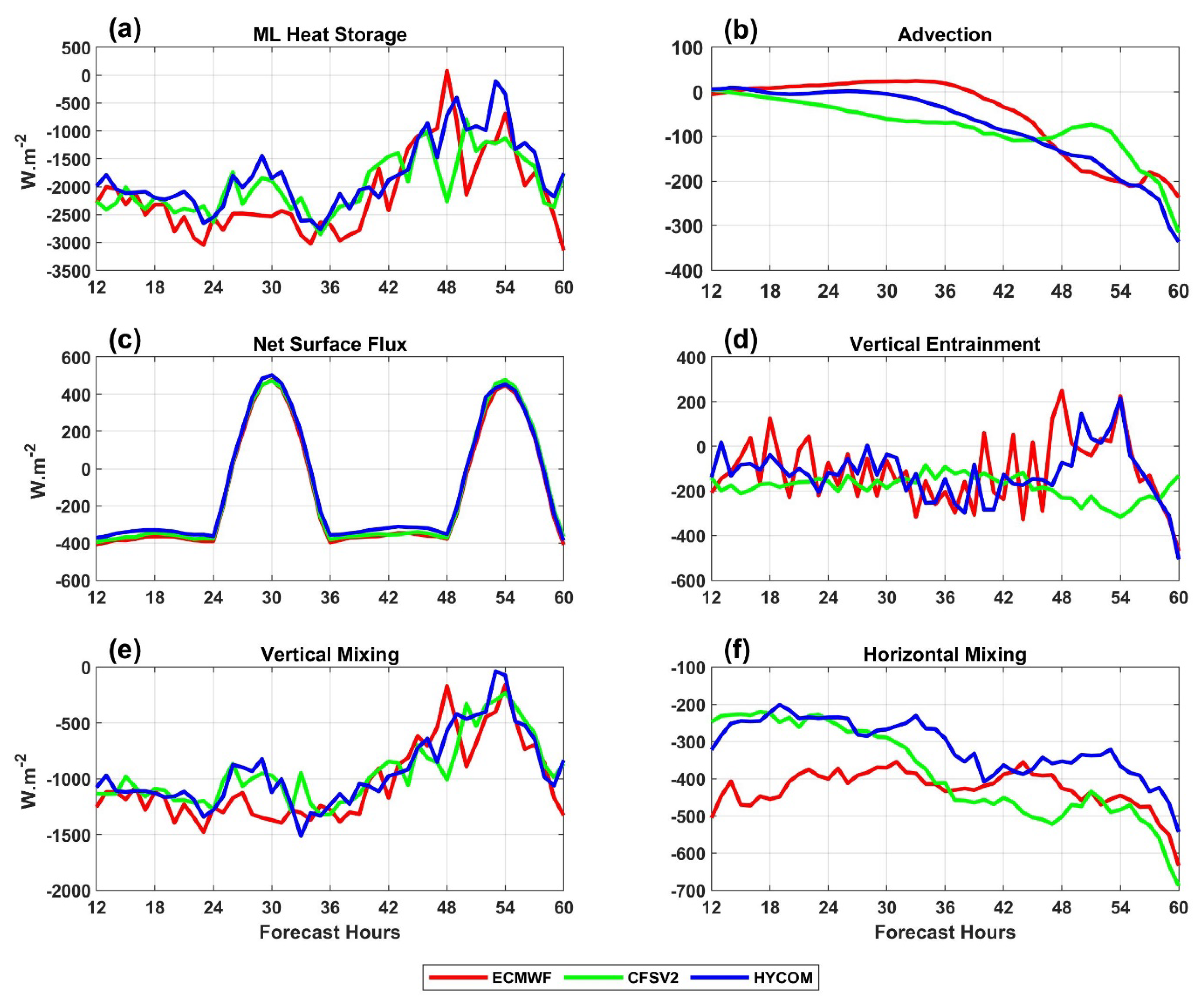
4.2.2. Mixed Layer Depth and Mixed Layer Heat Budget

The time series for the mixed layer depth (MLD) and mixed layer heat content (MLHC) are shown in Figure 7. The MLD is defined as the depth where the density is greater than the surface value by 0.125 kg.m⁻³ [13]. The MLHC was calculated using the formulation shown in Equation (1):

$$MLHC={{\displaystyle \int }}_0^{-h}\rho C_{p}Tdz$$

(1)

where $h=$ the MLD, $\rho$ = density, and $C_p=$ specific heat capacity of ocean water at constant pressure; T = temperature; and z corresponds to the depth. The integration was carried out over the depth, from z = 0 (surface) to z = −h (MLD). It can be seen that CFSV2 simulated a deeper mixed layer (ML) throughout the course of the simulation (Figure 7e). This is suggestive of higher mixing, which must have played an important role in hindering the intensification of the TC in CFSV2. However, the quadrant-wise segregation of MLD showed an interesting aspect. In the case of ECMWF, a sharp increase in the MLD could be seen in the NE quadrant (~50 m) between 30 and 42 h (Figure 7b) and in the SE quadrant (~40 m) between 42 and 54 h (Figure 7c). This was also reflected in the MLHC scenario (Figure 7g,h). These fluctuations in MLD occurred simultaneously with the SST variations, as discussed in the previous section.

After analysing the variations in the MLD and MLHC following the storm, it became extremely necessary to evaluate the contributions of the different processes to the evolution of the MLHC. Hence, to get a better understanding of the modulation of the MLHC by means of sub-surface processes, the MLHC budget was analyzed for all the experiments. The simplified version of the MLHC balance calculation (Equation (2) was implemented following the methodologies described by Foltz and McPhaden [77], Vijith et al. [78], and Vialard et al. [79]:

$$\underset{\begin{array}{c}\mathrm{ML} \mathrm{Heat} \\ \mathrm{Storage} \\ \mathrm{Rate}/\\ \mathrm{Tendency}\end{array}}{\underbrace{\rho C_p\hslash \frac{\partial T_a}{\partial t}}}=\underset{\mathrm{Advection}}{\underbrace{-\rho C_p\hslash (u_a\frac{\partial T_a}{\partial x}+v_a\frac{\partial T_a}{\partial y})}}-\underset{\begin{array}{c}\mathrm{Vertical} \\ \mathrm{Entrainment}\end{array}}{\underbrace{\rho C_p\hslash (\frac{T_a-T_h}{\hslash })(\frac{\partial h}{\partial t}+u_{\hslash }\frac{\partial h}{\partial x}+w_{\hslash })}}+\underset{\begin{array}{c}\mathrm{Net} \\ \mathrm{Surface} \\ \mathrm{Flux}\end{array}}{\underbrace{(q_0-q_{pen})}}+\underset{\begin{array}{c}\mathrm{Horizontal} \\ \mathrm{Mixing}\end{array}}{\underbrace{\rho C_p\hslash K_H(\frac{{\partial }^2{T}_a}{\partial x^2}+\frac{{\partial }^2{T}_a}{\partial y^2})}}-\underset{\begin{array}{c}\mathrm{Vertical} \\ \mathrm{Mixing}\end{array}}{\underbrace{\rho C_p[K_z\frac{\partial T}{\partial z}]}}\underset{\mathrm{Residua}l}{\underbrace{+R}}$$

(2)

The left-hand side of Equation (2) represents the ML heat storage term; or, simply, the temporal tendency of the MLHC. The first and second terms on the right-hand side (RHS) of the equation represent advection and vertical entrainment, respectively. The negative signs in these terms represent sink terms. The third term on the RHS represents the net surface flux. Here, $q_0=q_{SW}+q_{LW}+q_L+q_S$, where $q_{SW}$ = net surface shortwave flux, $q_{LW}$ = net surface longwave flux, $q_L$ = net surface latent heat flux, and $q_S$ = net surface sensible heat flux. The term $q_{pen}$ indicates that penetrating shortwave radiation below the mixed layer and was estimated following the methodology described by Morel and Antoine [80] and Sweeney et al. [81]. The fourth and fifth terms represent the horizontal and vertical mixing, respectively. K_Z and K_H indicate the vertical and horizontal eddy diffusivity, respectively.

The temporal variations in the different terms of the MLHC budget are shown in Figure 8. The residual term (consisting of unresolved processes, with values ranging from −1223.8 to 939 W·m⁻² for ECMWF, −983.53 to 947.42 W·m⁻² for CFSV2, and −925.52 to 847.94 W·m⁻² for HYCOM) is not shown, as the terms relevant for the discussion associated with the MLHC budget are already shown in Figure 8. It can be seen that the ML lost heat throughout the duration of the simulation for all three experiments. The rate of heat loss was higher in ECMWF for the initial hours. However, the rate of heat loss decreased more in ECMWF and HYCOM than in CFSV2 after 42 h (Figure 8a). The net surface flux showed diurnal variations and impacted the ML heat storage rate significantly in all three experiments. The horizontal mixing term contributed significantly to the ML heat storage in the initial hours. However, the term became dominating in CFSV2 after 36 h, at which point the heat loss due to horizontal mixing decreased in ECMWF and CFSV2 up to 45 h. The advection term showed a decreasing trend in all three experiments (Figure 8b). In addition, the vertical entrainment term showed an interesting variation between 36 and 54 h. The maximum loss in the MLHC due to entrainment occurred in CFSV2 (240–280 W·m⁻²). Investigation of the quadrant-wise variation in the entrainment term showed that an addition of heat to the ML in the NE quadrant occurred in ECMWF between 42 and 54 h (Figure 9g), which was simultaneous with the rising pattern seen for the heat storage term in the NE quadrant in ECMWF (Figure 9b) compared to the other two experiments.

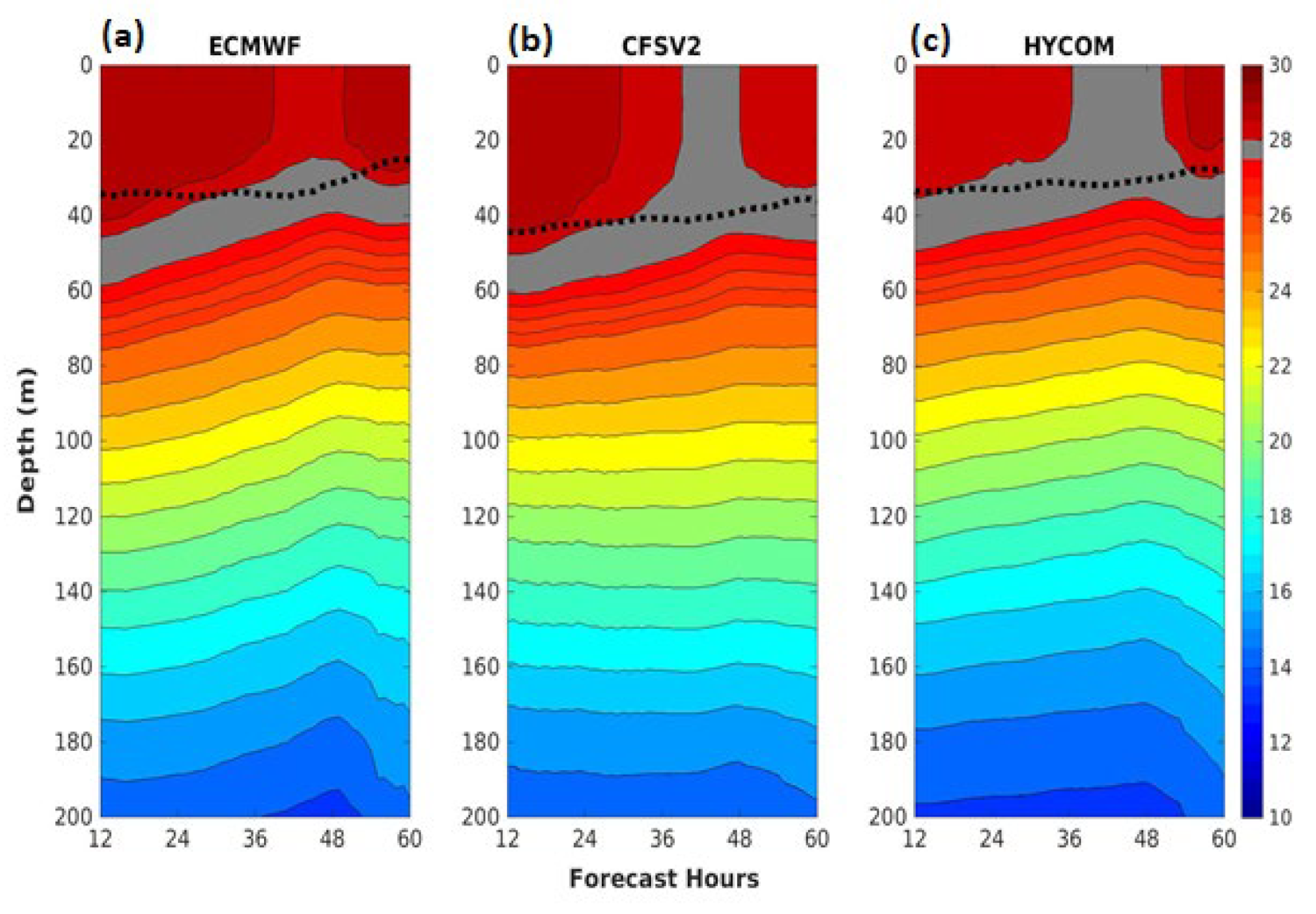
4.2.3. Vertical Variations in Temperature and Upwelling

Figure 10 shows the vertical profile for the ocean sub-surface temperature up to the depth of 200 m, overlaid with the temporal variations in the MLD calculated over the VFB. The steep curvature of the isotherms after 36 h indicated that upwelling was taking place under the storm core. From the curvature of the isotherms, it can be inferred that ECMWF (CFSV2) had the most rigorous (weakest) upwelling (Figure 10a,b). Another interesting point that can be noted from the results is that colder ocean water from depth reached the surface in CFSV2 (Figure 10b) and HYCOM (Figure 10c), which did not happen in the case of ECMWF. In ECMWF, the upwelling did not change the temperature distribution in the ML, as the colder water from the depths did not reach the surface (Figure 10a). This indicates that, though the upwelling of water was prevalent in ECMWF, the rising of water occurred from shallower depths, possibly from the barrier layer region. CFSV2 simulated a deeper mixed layer, suggesting higher mixing, which hindered the TC intensification. Further, there was a notable change in the MLD, other than the decreasing trend seen throughout the simulation in CFSV2 (Figure 10b). However, a completely different picture was seen in ECMWF. It can be noted that there was a massive steepening of the MLD at around 40 h, which was simultaneous with the enhanced upwelling. This phenomenon was not seen in the other two experiments.

To understand the upwelling scenario better, the pre-existing upwelling conditions were investigated. Figure 11 shows the simulated sea surface height anomaly (SSHA); tracks are overlaid with the surface geostrophic current averaged from the initial 24 h of the simulations, and forecasted tracks for all three experiments were validated against SSHA data obtained from the Copernicus Climate Change Services (C3S, horizontal resolution of 0.25°), which were overlaid with the Copernicus Marine Environment Monitoring Services (CMEMS) geostrophic current observations and the IMD track (Figure 11a). In addition, the positions of the cyclones (both observed and simulated) at 48 h and 54 h are shown using the green and blue markers, respectively. It should be noted that negative values for the SSHA are an indicator of upwelling conditions and an existing cold-core system. It is evident from the C3S observations that a cold-core eddy existed between 16.5–18.5° N over which the TC passed (Figure 11a). This cold-core eddy structure was reasonably captured in ECMWF (Figure 11b) and HYCOM (Figure 11d), but it was completely absent in CFSV2 (Figure 11c). Furthermore, ECMWF simulated a stronger geostrophic current than HYCOM. When a TC interacts with such a cold-core eddy system, the upwelling is enhanced, and exactly this was seen in ECMWF and, to some extent, in HYCOM. However, the absence of the cold-core eddies in CFSV2 indicated that the upwelling was solely due to vortex-induced winds.

4.2.4. Barrier Layer

As the findings from the previous analyses highlighted the possible presence or absence of the BL in the experiments, such as the addition of heat to the mixed layer by means of vertical entrainment in ECMWF and cold water being prevented from reaching the surface in ECMWF in spite of the presence of enhanced upwelling, the identification of the contribution of the barrier layer to the modulation of ocean sub-surface processes was judged to be necessary. Hence, the BL thickness (BLT) was calculated following the methodology described by Balaguru et al. [41] with the following equation:

$$\mathrm{BLT}=\mathrm{ILD}-\mathrm{MLD}$$

(3)

where ILD is the isothermal layer depth [82]. Figure 12 shows the evolution of the BLT over the BoB from the initial time of the simulation up to 48 h with intervals of 24 h for all three experiments. It can be clearly seen that the values of the BLT along the passage of the simulated TC were highest in ECMWF (up to 60 m) throughout the simulation, followed by HYCOM (up to 50 m). However, as anticipated, the BLT was lowest in CFSV2 (~15–20 m). Hence, Figure 11 corroborates the indications obtained from the previous analyses. The simulated TC passed over a zone of high BLT in ECMWF before making landfall (Figure 12a,d,g). This contributed to the intensification of the TC in that simulation by preventing the intrusion of cold water from the depths into the mixed layer. This was also observed in HYCOM to some extent, but the lower spatial spread of zones of high BLT minimized the contribution (Figure 12b,e,h). Finally, in CFSV2, due to the absence of a BL below the passage of the simulated TC, the cyclone-induced upwelling resulted in cold water reaching the surface, leading to the decay of intensification processes.

5. Summary and Conclusions

The basic characteristics of ocean sub-surface processes, along with their impact on the intensification process of TC Phailin, were investigated using the COAWST modeling framework with three sub-surface ocean conditions; viz., ECMWF, CFSV2, and HYCOM. In terms of MCP and M10SW, ECMWF simulated the most intense TC, closer to the IMD data. However, all the simulations showed a delay in the intensification of the TC. The radius-pressure cross-section of the DH, the TW, and the radial distribution of radar reflectivity confirmed that all the experiments simulated an axisymmetric TC. However, from the inner core structure of the DH and TW, it was also evident that ECMWF (CFSV2) captured the strongest (weakest) inner core of the TC, modulating its intensification. This resulted in ECMWF simulating the most intense storm among the three experiments.

The deeper ML in CFSV2 throughout the course of the simulation indicated the domination of mixing, which in turn hindered the intensification of the TC in that simulation. However, in ECMWF, a sudden and distinct increase in the MLD was noted in the NE quadrant, facilitating a simultaneous increase in the MLHC between 30 and 42 h. To understand its consequences, an MLHC budget calculation was carried out. The vertical entrainment term showed that the highest loss in MLHC due to entrainment occurred in CFSV2, indicating a greater amount of cold-water intrusion within the ML. Furthermore, in ECMWF, the vertical entrainment in the NE quadrant supplied additional heat to the ML between 36 and 42 h, which occurred in tandem with the sudden increase in the MLD over the NE quadrant. It can be seen from the vertical distribution of the temperature that cold water from the depths reached the surface in CFSV2 and HYCOM but not in ECMWF. This justified the greater reduction in SST in the NE and SE quadrants (with the SE quadrant lagging behind the NE quadrant by around 6 h) in CFSV2 and HYCOM compared to ECMWF. Enhanced upwelling was noted in ECMWF and, to some extent, in HYCOM, as they were able to simulate the TC’s interactions with the pre-existing cold-core eddy situated between 16.5–18.5° N during its passage for the period between 42 and 54 h of the simulations. CFSV2 failed to capture these features of enhanced upwelling, which, on the one hand, can be attributed to the coarser resolution of the ocean datasets and, on the other hand, can be justified by the different data assimilation procedures and observations used in the assimilation of said dataset.

As the freshwater input to the BoB increases during the monsoon season due to excess river runoff and enhanced seasonal precipitation, the salinity profile becomes more stratified, resulting in the occasional formation of barrier layers in the post-monsoon season. When TCs pass over these regions with barrier layers, they tend to intensify as cyclone-induced upwelling breaks the barrier layer and brings warm water into the ML, resulting in a change in the distribution of the MLHC and subsequent modulation of SST and enthalpy fluxes [41]. In the case of ECMWF, it was seen that there was a sudden increase in the MLD between 36 and 42 h in the NE quadrant, with the simultaneous addition of heat in the ML due to vertical entrainment. Furthermore, despite the passage of the simulated TC over a cold-core eddy, which is supposed to weaken the storm core by means of upwelling of the cold water from the depths, it was seen that the temperature distribution of the ML was unaffected, as cold water from the depths was prevented from reaching the surface in ECMWF. As shown in previous studies [83,84], these pieces of evidence suggest that cyclone-induced upwelling and the enhanced upwelling caused by the interaction with the cold-core eddy caused the breaking of the barrier layer in the NE quadrant of the TC in ECMWF, enabling it to simulate a more intense and realistic TC than the other two experiments. This is further corroborated by the spatial distribution of the BLT seen in the three experiments. The absence of a barrier layer and transport of deeper cold water to the surface due to cyclone-induced upwelling caused a decrease in SST in CFSV2 and, to some extent, HYCOM, which acted as a negative feedback mechanism, hindering the intensification and resulting in the simulation of a relatively weaker TC. However, since the NE quadrant of the VFB was partially over the warm-core eddy situated beside the cold-core eddy, this possibly impacted the SST and enthalpy flux scenario to some extent. The detailed mechanism is schematically depicted in Figure 13. Finally, to summarize, the findings of the study are listed below in bullet points:

• Among the three simulations, ECMWF was able to capture the intensity of TC Phailin with the highest accuracy. Analysis of the DH and TW also suggested that ECMWF simulated the strongest inner-core structure for the TC;
• In the case of ECMWF, an increase in the MLD was observed between 30 and 42 h and, simultaneously, addition of heat to the mixed layer took place by means of vertical entrainment. This was also visible in the case of HYCOM to some extent but not in CFSV2;
• ECMWF and HYCOM replicated the cold-core eddy structure in the east-central BoB in accordance with observations, but CFSV2 failed to capture this feature. Further, the passage of the TC over the cold-core eddy did not hamper the intensification of the TC in ECMWF;
• Despite the enhanced upwelling, cold water from the depths did not reach the surface in ECMWF, unlike in CFSV2 and HYCOM. This meant that the SST distribution was not reduced under the storm in ECMWF, which favored the intensification in that simulation;
• Prevention of cold water reaching the surface was facilitated by the presence of a BL in ECMWF. Upwelling induced by TC circulation and a cold-core eddy caused the breaking of the BL, which modulated the MLHC and acted as positive feedback for TC intensification in ECMWF.

Previous studies [34] have discussed the evolution of the temperature and heat content in the ML after the passage of a TC. However, instead of the ocean responses after the passage of a TC, the ocean–atmosphere interactions during the passage of the cyclone were emphasized in this study. It was also demonstrated in earlier studies that the interaction of TCs with warm-core eddies has a significant impact on their intensification, and TC interaction with cold-core eddies leads to the weakening of TC strength [39,40]. However, this study concluded that passage of a cyclone over a cold-core eddy does not necessarily weaken it, as enhanced upwelling caused by the cold-core eddy can break the BL and contribute to the strength of the TC by modulating the MLHC. The findings of this study strengthen the idea that the coupled modeling approach is essential to understand the sub-surface ocean mechanisms and predict the intensification processes of TCs accurately, and they also demonstrate the capacity of the coupled model to capture barrier layer-associated processes and their influence on the intensification of TCs. In addition, this study demonstrates that the presence or absence of a BL in the oceanic datasets used for the simulation of post-monsoon TCs over the BoB basin has a significant impact on the outcome of the simulations. Furthermore, proper representation of prevailing mesoscale features, as well as the temperature and salinity distribution in the ocean’s initial and boundary conditions, are essential for a realistic simulation. This study can be used as a benchmark for understanding sub-surface ocean influences on the intensification of TCs originating in the post-monsoon season over the BoB. However, further analysis of energetics will help us understand the coupled feedback with more clarity.

References

1. Alam, M.M.; Hossain, M.A.; Shafee, S. Frequency of Bay of Bengal Cyclonic Storms and Depressions Crossing Different Coastal Zones. Int. J. Climatol. 2003, 23, 1119–1125. [Google Scholar] [CrossRef]
2. Emanuel, K.A. Thermodynamic control of hurricane intensity. Nature 1999, 401, 665–669. [Google Scholar] [CrossRef]
3. Marks, F.; Shay, L.K. Landfalling tropical cyclones: Forecast problems and associated research opportunities: Report of the 5th prospectus development team to the US Weather Research Program. Bull. Am. Meteorol. Soc. 1998, 79, 305–323. [Google Scholar]
4. Riehl, H. A model of hurricane formation. J. App. Phys. 1950, 21, 917–925. [Google Scholar] [CrossRef]
5. Emanuel, K.A. The dependence of hurricane intensity on climate. Nature 1987, 326, 483–485. [Google Scholar] [CrossRef]
6. Gray, W.M. The formation of tropical cyclones. Meteorol. Atmos. Phys. 1998, 67, 37–69. [Google Scholar] [CrossRef]
7. Miller, B.I. On the maximum intensity of hurricanes. J. Atmos. Sci. 1958, 15, 184–195. [Google Scholar] [CrossRef] [Green Version]
8. Mandal, M.; Mohanty, U.C.; Sinha, P.; Ali, M.M. Impact of sea surface temperature in modulating movement and intensity of tropical cyclones. Nat. Hazards 2007, 41, 413–427. [Google Scholar] [CrossRef]
9. Rai, D.; Pattnaik, S.; Rajesh, P.V. Sensitivity of Tropical Cyclone Characteristics to the Radial Distribution of Sea Surface Temperature. J. Earth Syst. Sci. 2016, 125, 691–708. [Google Scholar] [CrossRef] [Green Version]
10. Vishwakarma, V.; Pattnaik, S.; Chakraborty, T.; Joseph, S.; Mitra, A.K. Impacts of sea-surface temperatures on rapid intensification and mature phases of super cyclone Amphan (2020). J. Earth Syst. Sci. 2022, 131, 60. [Google Scholar] [CrossRef]
11. Yun, K.; Chan, J.C.L.; Ha, K. Effects of SST magnitude and gradient on typhoon tracks around east Asia: A case study for typhoon Maemi (2003). Atmos. Res. 2012, 109–110, 36–51. [Google Scholar] [CrossRef]
12. Shenoi, S.S.C.; Shankar, D.; Shetye, S.R. Differences in heat budgets of the near-surface Arabian Sea and Bay of Bengal: Implications for the summer monsoon. J. Geophys. Res. 2002, 107, 1–14. [Google Scholar] [CrossRef]
13. Rao, R.R.; Sivakumar, R. Seasonal variability of sea surface salinity and salt budget of the mixed layer of the north Indian Ocean. J. Geophys. Res. 2003, 108, 3009. [Google Scholar] [CrossRef]
14. Thadathil, P.; Muraleedharan, P.M.; Rao, R.R.; Somayajulu, Y.K.; Reddy, G.V.; Revichandran, C. Observed seasonal variability of barrier layer in the Bay of Bengal. J. Geophys. Res. 2007, 112, C02009. [Google Scholar] [CrossRef]
15. Girishkumar, M.S.; Ravichandran, M.; Han, W. Observed intraseasonal thermocline variability in the Bay of Bengal. J. Geophys. Res. Oceans 2013, 118, 3336–3349. [Google Scholar] [CrossRef]
16. Schade, L.R. Tropical Cyclone Intensity and Sea Surface Temperature. J. Atmos. Sci. 2000, 57, 3122–3130. [Google Scholar] [CrossRef]
17. Price, J.F. Upper-ocean response to a hurricane. J. Phys. Oceanogr. 1981, 11, 153–175. [Google Scholar] [CrossRef] [Green Version]
18. Bender, M.A.; Ginis, I.; Kurihara, Y. Numerical simulations of the tropical cyclone-ocean interaction with a high-resolution coupled model. J. Geophys. Res. 1993, 98, 23245–23263. [Google Scholar] [CrossRef]
19. Schade, L.R.; Emanuel, K.A. The ocean’s effect on the intensity of tropical cyclones: Results from a simple coupled atmosphere-ocean model. J. Atmos. Sci. 1994, 56, 642–651. [Google Scholar] [CrossRef] [Green Version]
20. Bosart, L.; Velden, C.S.; Bracken, W.E.; Molinari, J.; Black, P.G. Environmental influences on the rapid intensification of Hurricane Opal (1995) over the Gulf of Mexico. Mon. Weather Rev. 2000, 128, 322–352. [Google Scholar] [CrossRef]
21. Chan, J.C.L.; Duan, Y.; Shay, L.K. Tropical cyclone intensity change from a simple ocean-atmosphere coupled model. J. Atmos. Sci. 2001, 58, 154–172. [Google Scholar] [CrossRef]
22. Lin, Y.L.; Chen, S.Y.; Hill, C.M.; Huang, C.Y. Control parameters for the influence of a mesoscale mountain range on cyclone track continuity and deflection. J. Atmos. Sci. 2005, 62, 1849–1866. [Google Scholar] [CrossRef]
23. Ali, M.M.; Kashyap, T.; Nagamani, P.V. Use of Sea Surface Temperature for Cyclone Intensity Prediction Needs a Relook. EOS Trans. Am. Geophys. Union 2013, 94, 177. [Google Scholar] [CrossRef]
24. Vissa, N.K.; Satyanarayana, A.N.V.; Prasad, K.B. Response of upper ocean during passage of MALA cyclone utilizing ARGO data. Int. J. Appl. Earth Obs. Geoinfo. 2012, 14, 149–159. [Google Scholar] [CrossRef]
25. Mohan, G.M.; Srinivas, C.V.; Naidu, C.V.; Baskaran, R.; Venkatraman, B. Real-time numerical simulation of tropical cyclone Nilam with the WRF: Experiments with different initial conditions, 3D-Var and Ocean Mixed Layer Model. Nat. Hazards 2015, 77, 597–624. [Google Scholar] [CrossRef]
26. Leipper, D.; Volgenau, D. Upper ocean heat content of the Gulf of Mexico. J. Phys. Oceanogr. 1972, 2, 218–224. [Google Scholar] [CrossRef]
27. Sadhuram, Y.; Ramana Murthy, T.V.; Somayajulu, Y.K. Estimation of tropical cyclone heat potential in the Bay of Bengal and its role in the genesis and intensification of storms. Indian J. Mar. Sci. 2006, 352, 132–138. [Google Scholar]
28. Vissa, N.K.; Satyanarayana, A.N.V.; Prasad, K.B. Response of upper ocean and impact of barrier layer on Sidr cyclone induced sea surface cooling. Ocean Sci. J. 2013, 48, 279–288. [Google Scholar] [CrossRef]
29. Li, D.-Y.; Huang, C.-Y. The influences of ocean on intensity of typhoon Soudelor (2015) as revealed by coupled modeling. Atmos. Sci. Lett. 2019, 20, e871. [Google Scholar] [CrossRef]
30. Tada, H.; Uchiyama, Y.; Masunaga, E. Impacts of two super typhoons on the Kuroshio and marginal seas on the Pacific coast of Japan. Deep-Sea Res. Part I Oceanogr. Res. Pap. 2018, 132, 80–93. [Google Scholar] [CrossRef]
31. Davis, C.; Wang, W.; Chen, S.S.; Chen, Y.; Corbosiero, K.; DeMaria, M.; Dudhia, J.; Holland, G.; Klemp, J.; Michalakes, J.; et al. Prediction of Landfalling Hurricanes with the Advanced Hurricane WRF Model. Mon. Weather Rev. 2008, 136, 1990–2005. [Google Scholar] [CrossRef] [Green Version]
32. Wu, C.C.; Tu, W.T.; Pun, I.F.; Lin, I.I.; Peng, M.S. Tropical cyclone-ocean interaction in Typhoon Megi (2010)—A synergy study based on ITOP observations and atmosphere-ocean coupled model simulations. J. Geophys. Res. Atmos. 2016, 121, 153–167. [Google Scholar] [CrossRef]
33. Zhao, X.; Chan, J.C.L. Changes in tropical cyclone intensity with translation speed and mixed-layer depth: Idealized WRF-ROMS coupled model simulations. Q. J. R. Meteorol. Soc. 2016, 143, 152–163. [Google Scholar] [CrossRef]
34. Prakash, K.R.; Pant, V. Upper oceanic response to tropical cyclone Phailin in the Bay of Bengal using a coupled atmosphere-ocean model. Ocean Dyn. 2017, 67, 51–64. [Google Scholar] [CrossRef]
35. Mogensen, K.S.; Magnusson, L.; Bidlot, J.R. Tropical cyclone sensitivity to ocean coupling in the ECMWF coupled model. J. Geophys. Res. Oceans 2017, 122, 4392–4412. [Google Scholar] [CrossRef]
36. Yesubabu, V.; Kattamanchi, V.K.; Vissa, N.K.; Dasari, H.P.; Sarangam, V.B.R. Impact of ocean mixed-layer depth initialization on the simulation of tropical cyclones over the Bay of Bengal using the WRF-ARW model. Meteorol. Appl. 2019, 27, e1862. [Google Scholar] [CrossRef]
37. Baisya, H.; Pattnaik, S.; Chakraborty, T. A coupled modeling approach to understand ocean coupling and energetics of tropical cyclones in the Bay of Bengal basin. Atmos. Res. 2020, 246, 105092. [Google Scholar] [CrossRef]
38. Li, Z.; Tam, C.-Y.; Li, Y.; Lau, N.-C.; Chen, J.; Chan, S.T. How does air-sea wave interaction affect tropical cyclone intensity? An atmosphere-wave-ocean coupled model study based on super typhoon Mangkhut (2018). Earth Space Sci. 2022, 9, e2021EA002136. [Google Scholar] [CrossRef]
39. Anandh, T.S.; Das, B.K.; Kuttipurath, J.; Chakraborty, A. A coupled model analyses on the interaction between oceanic eddies and tropical cyclones over the Bay of Bengal. Ocean Dyn. 2020, 70, 327–337. [Google Scholar] [CrossRef]
40. Sun, J.; Wang, G.; Xiong, X.; Hui, Z.; Hu, X.; Ling, Z.; Long, Y.; Yang, G.; Guo, Y.; Ju, X.; et al. Impact of warm mesoscale eddy on tropical cyclone intensity. Acta Oceanol. Sin. 2020, 39, 1–13. [Google Scholar] [CrossRef]
41. Balaguru, K.; Chang, P.; Saravanan, R.; Leung, L.R.; Xu, Z.; Li, M.; Hsieh, J.S. Ocean barrier layers’ effect on tropical cyclone intensification. Proc. Natl. Acad. Sci. USA 2012, 109, 14343–14347. [Google Scholar] [CrossRef] [Green Version]
42. Rudzin, J.E.; Shay, L.K.; Johns, W.E. The Influence of the Barrier Layer on SST Response during Tropical Cyclone Wind Forcing Using Idealized Experiments. J. Phys. Oceanogr. 2018, 48, 1471–1478. [Google Scholar] [CrossRef]
43. Cyclone Warning Division, India Meteorological Department. Very Severe Cyclonic Storm, Phailin over the Bay of Bengal (08-14 October 2013): A Report. 2013. Available online: www.rsmcnewdelhi.imd.gov.in/uploads/report/26/26_38a1d4_phailin.pdf (accessed on 8 January 2022).
44. Warner, J.C.; Armstrong, B.; He, R.; Zambon, J.B. Development of a Coupled Ocean–Atmosphere–Wave–Sediment Transport (COAWST) Modeling System. Ocean Mod. 2010, 35, 230–244. [Google Scholar] [CrossRef] [Green Version]
45. Skamarock, W.C.; Klemp, J.B.; Dudhia, J.; Gill, D.O.; Barker, D.M.; Duda, M.G.; Huang, X.Y.; Wang, W.; Powers, J.G. A Description of the Advanced Research WRF Version 3; Technical Report; National Center for Atmospheric Research: Boulder, CO, USA, 2008. [Google Scholar]
46. Shchepetkin, A.F.; McWilliams, J.C. The regional oceanic modeling system (ROMS): A split-explicit, free-surface, topography-following-coordinate oceanic model. Ocean Mod. 2005, 9, 347–404. [Google Scholar] [CrossRef]
47. Haidvogel, D.B.; Arango, H.; Budgell, W.P.; Cornuelle, B.D.; Curchitser, E.; Di Lorenzo, E.; Fennel, K.; Geyer, W.R.; Hermann, A.J.; Lanerolle, L.; et al. Ocean forecasting in terrain-following coordinates: Formulation and skill assessment of the Regional Ocean Modeling System. J. Comput. Phys. 2008, 227, 3595–3624. [Google Scholar] [CrossRef]
48. Booij, N.; Ris, R.C.; Holthuijsen, L.H. A third-generation wave model for coastal regions: 1. Model description and validation. J. Geophys. Res. Oceans 1999, 104, 7649–7666. [Google Scholar] [CrossRef] [Green Version]
49. Warner, J.C.; Sherwood, C.R.; Signell, R.P.; Harris, C.K.; Arango, H.G. Development of a three-dimensional, regional, coupled wave, current, and sediment-transport model. Comput. Geosci. 2008, 34, 1284–1306. [Google Scholar] [CrossRef]
50. Larson, J.; Jacob, R.; Ong, E. The Model Coupling Toolkit: A New Fortran90 Toolkit for Building Multiphysics Parallel Coupled Models. Int. J. High Perform. Comput. Appl. 2005, 19, 277–292. [Google Scholar] [CrossRef]
51. Jacob, R.; Larson, J.; Ong, E. M × N Communication and Parallel Interpolation in Community Climate System Model Version 3 Using the Model Coupling Toolkit. Int. J. High Perform. Comput. Appl. 2005, 19, 293–307. [Google Scholar] [CrossRef]
52. Jones, P.W. First- and Second-Order Conservative Remapping Schemes for Grids in Spherical Coordinates. Mon. Weather Rev. 1999, 127, 2204–2210. [Google Scholar] [CrossRef]
53. Saha, S.; Moorthi, S.; Pan, H.-L.; Wu, X.; Wang, J.; Nadiga, S.; Tripp, P.; Kistler, R.; Woollen, J.; Behringer, D.; et al. NCEP Climate Forecast System Reanalysis (CFSR) 6-hourly Products, January 1979 to December 2010; Research Data Archive at the National Center for Atmospheric Research, Computational and Information Systems Laboratory: Boulder, CO, USA, 2010. [CrossRef]
54. Drévillon, M.; Regnier, C.; Lellouche, J.M.; Garric, G.; Bricaud, C.; Hernandez, O. CMEMS-GLO-QUID-001-030, 1.2 edn. E.U. Copernicus Marine Service Information. 2018. Available online: https://resources.marine.copernicus.eu/documents/QUID/CMEMS-GLO-QUID-001-030.pdf (accessed on 17 December 2021).
55. Chassignet, E.P.; Smith, L.T.; Halliwell, G.R.; Bleck, R. North Atlantic Simulations with the Hybrid Coordinate Ocean Model (HYCOM): Impact of the Vertical Coordinate Choice, Reference Pressure, and Thermobaricity. J. Phys. Oceanogr. 2003, 33, 2504–2526. [Google Scholar] [CrossRef] [Green Version]
56. Egbert, G.D.; Erofeeva, G.D. Effective Inverse Modeling of Barotropic Ocean Tides. J. Atmos. Ocean. Technol. 2002, 19, 183–204. [Google Scholar] [CrossRef] [Green Version]
57. Lim, K.-S.S.; Hong, S.-Y. Development of an effective double-moment cloud microphysics scheme with prognostic cloud condensation nuclei (CCN) for weather and climate models. Mon. Weather Rev. 2010, 139, 1013–1035. [Google Scholar] [CrossRef] [Green Version]
58. Chou, M.-D.; Suarez, M.J. Technical Report Series on Global Modeling and Data Assimilation, Volume 15: A Solar Radiation Parameterization for Atmospheric Studies; NASA Technology Report NASA/TM-1999-10460; NASA: Washington, DC, USA, 1999; Volume 15.
59. Mlawer, E.J.; Taubman, S.J.; Brown, P.D.; Iacono, M.J.; Clough, S.A. Radiative transfer for inhomogeneous atmospheres: RRTM, a validated correlated-k model for the longwave. J. Geophys. Res. 1997, 102, 16663. [Google Scholar] [CrossRef] [Green Version]
60. Zhang, D.; Anthes, R.A. A High-Resolution Model of the Planetary Boundary Layer-Sensitivity Tests and Comparisons with SESAME-79 Data. J. Appl. Meteorol. 1982, 21, 1594–1609. [Google Scholar] [CrossRef]
61. Ek, M.B. Implementation of Noah Land Surface Model Advances in the National Centres for Environmental Prediction Operational Mesoscale Eta Model. J. Geophys. Res. 2003, 108, 8851. [Google Scholar] [CrossRef]
62. Hong, S.-Y.; Noh, Y.; Dudhia, J. A new vertical diffusion package with an explicit treatment of entrainment processes. Mon. Weather Rev. 2006, 134, 2318–2341. [Google Scholar] [CrossRef] [Green Version]
63. Kain, J.S. The Kain-Fritsch Convective Parameterization: An Update. J. App. Meteorol. 2004, 43, 170–181. [Google Scholar] [CrossRef] [Green Version]
64. Taylor, P.K.; Yelland, M.J. The Dependence of Sea Surface Roughness on the Height and Steepness of the Waves. J. Phys. Oceanogr. 2001, 31, 572–590. [Google Scholar] [CrossRef] [Green Version]
65. Uchiyama, Y.; McWilliams, J.C.; Shchepetkin, A.F. Wave-current interaction in an oceanic circulation model with vortex-force formalism: Application to the surf zone. Ocean Mod. 2010, 34, 16–35. [Google Scholar] [CrossRef]
66. Kirby, J.T.; Chen, T.-M. Surface waves on vertically sheared flows: Approximate dispersion relations. J. Geophys. Res. 1989, 94, 1013. [Google Scholar] [CrossRef] [Green Version]
67. Warner, J.C.; Sherwood, C.R.; Arango, H.G.; Signell, R.P. Performance of four turbulence closure models implemented using a generic length scale method. Ocean Mod. 2005, 8, 81–113. [Google Scholar] [CrossRef]
68. Madsen, O.S.; Poon, Y.-K.; Graber, H.C. Spectral Wave Attenuation by Bottom Friction: Theory. Coast. Eng. Proc. 1989, 1, 34. [Google Scholar] [CrossRef]
69. Komen, G.J.; Hasselmann, K. On the existence of a fully developed wind-sea spectrum. J. Phys. Oceanogr. 1984, 14, 1271–1285. [Google Scholar] [CrossRef]
70. Climate Prediction Center/National Centers for Environmental Prediction/National Weather Service/NOAA/US Department of Commerce. NOAA CPC Morphing Technique (CMORPH) Global Precipitation Anlyses; Research Data Archive at the Center for Atmospheric Research, Computational and Information Systems Laboratory: Boulder, CO, USA, 2011.
71. Wilks, D.S. Statistical methods in the atmospheric sciences. Int. Geophys. 2011, 100, 2–76. [Google Scholar]
72. Vigh, J.L.; Schubert, W.H. Rapid development of the tropical cyclone warm core. J. Atmos. Sci. 2009, 66, 3335–3350. [Google Scholar] [CrossRef] [Green Version]
73. Stern, D.P.; Nolan, W.H. Reexamining the vertical structure of tangential winds in tropical cyclones: Observations and theory. J. Atmos. Sci. 2009, 66, 3579–3600. [Google Scholar] [CrossRef] [Green Version]
74. Li, Q.; Wamg, Y.; Duan, Y. Effects of Diabatic Heating and Cooling in the Rapid Filamentation Zone on Structure and Intensity of a Simulated Tropical Cyclone. J. Atmos. Sci. 2014, 71, 3144–3163. [Google Scholar] [CrossRef]
75. Rai, D.; Pattnaik, S. Sensitivity of Tropical Cyclone Intensity and Structure to Planetary Boundary Layer Parameterization. Asia-Pac. J. Atmos. Sci. 2018, 54, 473–488. [Google Scholar] [CrossRef]
76. Good, S.A.; Embury, O.; Bulgin, C.E.; Mittaz, J. ESA Sea Surface Temperature Climate Change Initiative (SST_cci): Level 4 Analysis Climate Data Record, Version 2.1; Centre for Environmental Data Analysis: Chilton, UK, 2019. [Google Scholar] [CrossRef]
77. McPhaden, M.J.; Foltz, G.R.; Lee, T.; Murty, V.S.N.; Ravichandran, M.; Vecchi, G.A.; Vialard, J.; Wiggert, J.D.; Yu, L. Ocean–atmosphere interactions during cyclone Nargis. EOS Trans. Am. Geophys. Union 2009, 90, 53–54. [Google Scholar] [CrossRef]
78. Vijith, V.; Vinaychandran, P.N.; Webber, B.G.M.; Matthews, A.J.; George, J.V.; Kannaujia, V.K.; Lotliker, A.A.; Amol, P. Closing the sea surface mixed layer temperature budget from in situ observations alone: Operation Advection during BoBBLE. Sci. Rep. 2020, 10, 7062. [Google Scholar] [CrossRef] [PubMed]
79. Vialard, J.; Foltz, G.R.; McPhaden, M.J.; Duvel, J.P.; Montegut, C.B. Strong Indian Ocean sea surface temperature signals associated with the Madden-Julian Oscillation in late 2007 and early 2008. Geophys. Res. Lett. 2008, 35, L19608. [Google Scholar] [CrossRef] [Green Version]
80. Morel, A.; Antoine, D. Heating rate within the upper ocean in relation to its bio-optical state. J. Phys. Oceanogr. 1994, 24, 1652–1665. [Google Scholar] [CrossRef] [Green Version]
81. Sweeney, C.; Gnanadesikan, A.; Griffies, S.; Harrison, M.; Rosati, A.; Samuels, B. Impacts of shortwave penetration depth on large-scale ocean circulation heat transport. J. Phys. Oceanogr. 2005, 35, 1103–1119. [Google Scholar] [CrossRef] [Green Version]
82. Montegut, C.B.; Mignot, J.; Lazar, A.; Cravatte, S. Control of salinity on the mixed layer depth in the world ocean: 1. General description. J. Geophys. Res. Oceans 2007, 112, C06011. [Google Scholar] [CrossRef]
83. Chaudhuri, D.; Sengupta, D.; D’Asaro, E.; Venkatesan, R.; Ravichandran, M. Response of the Salinity-Stratified Bay of Bengal to Cyclone Phailin. J. Phys. Oceanogr. 2019, 49, 1121–1140. [Google Scholar] [CrossRef]
84. Dutta, D.; Mani, B.; Dash, M.K. Dynamic and thermodynamic upper-ocean response to the passage of Bay of Bengal cyclones ‘Phailin’ and ‘Hudhud’: A study using a coupled modelling system. Environ. Monit. Assess. 2019, 191, 808. [Google Scholar] [CrossRef]
Figure 1. The domains of the WRF, ROMS, and SWAN model (which is the same as the ROMS) in the simulations, along with the tracks simulated in the three experiments and the IMD best track (https://rsmcnewdelhi.imd.gov.in/report.php?internal_menu=MzM= (accessed on 8 January 2022)). The outer solid lines mark the boundaries for the WRF domain, whereas the solid line in the middle of the WRF domain marks the upper boundary of the ROMS and SWAN domain. The offset zooms into the region bounded by 13–28° N and 78–93° E to focus on the simulated and observed tracks.
Oceans 03 00025 g001
Figure 2. Time series of the (a) minimum central pressure (MCP, hPa) and (b) maximum 10 m sustained wind speed (M10SW, knots) for all the experiments, along with the IMD best estimates.
Oceans 03 00025 g002
Figure 3. Radial distribution (270 km) of the 24 h accumulated rainfall (mm) obtained from the experiments ((ac) ECMWF, (df) CFSV2, and (gi) HYCOM) and from CMORPH (jl).
Oceans 03 00025 g003
Figure 4. Azimuthally averaged pressure-radius distributions of diabatic heating (K·h−1. shading) and tangential wind (m·s−1, contour) for all three experiments ((ad) ECMWF, (eh) CFSV2, (il) HYCOM) at 12 h intervals between 24 and 60 h.
Oceans 03 00025 g004
Figure 5. Spatial distribution of SST (°C) as obtained from ESA CCI observations (ac) and the three experiments ((df) ECMWF, (gi) CFSV2, (jl) HYCOM) at 24 h intervals between 12 and 60 h.
Oceans 03 00025 g005
Figure 6. (aj) Time series of quadrant-wise variations in SST (°C) ((ae) NW, NE, SE, and SW quadrants and the total VFB. respectively) and enthalpy flux (W·m−2) ((fh) for the NW, NE, SE, and SW quadrants and the total VFB. respectively) calculated over the VFB from all the experiments.
Oceans 03 00025 g006
Figure 7. Time series for the quadrant-wise variations in (ae) mixed layer depth (MLD) (m) and (fj) mixed layer heat content (MLHC) (J·kg−1), calculated over the VFB, obtained from all the experiments.
Oceans 03 00025 g007
Figure 8. Time series for the different terms (W·m−2) (i.e., (a) mixed layer (ML) heat storage rate, (b) advection due to currents, (c) net surface radiation, (d) vertical entrainment, (e) vertical mixing, and (f) horizontal mixing) of the ML heat budget (calculated over the VFB) obtained from all the experiments.
Oceans 03 00025 g008
Figure 9. Quadrant-wise variations in the ML heat storage term (ae) and the vertical entrainment term (fj) (calculated over the VFB) obtained from the three experiments.
Oceans 03 00025 g009
Figure 10. Vertical profile for temperature (°C, shading) overlaid with the MLD (black dashed line) (calculated over the VFB) as obtained from the experiments. The region with temperatures between 27.8 and 28.4 °C is marked in gray.
Oceans 03 00025 g010
Figure 11. Spatial distribution of sea surface height anomalies (SSHA, shading) and geostrophic currents (vectors) from C3S (for SSHA) and CMEMS (for geostrophic currents) observations and from the experiments. The track observed by the IMD is shown with the C3S-observed SSHA, while the simulated tracks (black lines) are shown for each of the experiments. The positions of the TC at 48 h (green marker) and 54 h (blue marker) are also shown. The C3S observations were remapped at the resolution of the simulations.
Oceans 03 00025 g011
Figure 12. Spatial distribution of barrier layer thickness (BLT) at 00 h (ac), 24 h (df), and 48 h (gi) for all three experiments.
Oceans 03 00025 g012
Figure 13. Schematic of the ocean processes influencing the intensification of TC Phailin in the simulations.
Oceans 03 00025 g013