Article

Customized Orthosis Design Based on Surface Reconstruction from 3D-Scanned Points

1
Department of Mechanical Engineering, College of Engineering, Imam Mohammad Ibn Saud Islamic University (IMSIU), Riyadh 11432, Saudi Arabia
2
LMS and LATIS, ENISo and ISSATSo, University of Sousse, Sousse 4000, Tunisia
3
Department of Industrial Engineering, College of Engineering, King Saud University, Riyadh 11421, Saudi Arabia
*
Author to whom correspondence should be addressed.
Prosthesis 2024, 6(1), 93-106; https://doi.org/10.3390/prosthesis6010008
Submission received: 6 December 2023 / Revised: 8 January 2024 / Accepted: 11 January 2024 / Published: 24 January 2024

Abstract

:
Limb disability is a frequent healthcare problem, especially for patients in primary care. Orthotic treatment has become the most common practice for either rehabilitation or permanent assistance, due to the emergence of 3D scanning and 3D printing technologies. A CAD model rebuilt from captured data is a key step in the rapid prototyping process of customized orthoses. An accurate and robust surface reconstruction technique remains a research challenge, aiming for a well-fitting design and the patient’s comfort. Thus, this paper presents of a new 3D curve-based reconstruction algorithm to obtain a precise 3D surface of an orthotic device from a scanned body part. Numerical experiments of two orthosis design case studies are shown to evaluate the reliability and accuracy of the proposed approach compared to other reconstruction methods.

1. Introduction

According to the World Health Organization (WHO) [1], about 15% of the world’s population lives with some form of disability, of whom 2–4% experience significant difficulties with normal daily functions. There is an urgent need to scale up disability services in primary healthcare. Thus, limb disability is a global public health problem. There are various types of treatments for limb disabilities such as surgical, therapeutic, or orthotic.
Orthotic devices have been widely used not only to provide mobilization, support, correction, or protection, but also to treat musculoskeletal injuries or dysfunctions [2]. The traditional process of manufacturing customized orthoses is established manually depending on an orthotic technician’s skills [3]. Plaster cast-based orthoses can cause patients discomfort due to the device’s heavy weight, bad air circulation, the requirement to keep it dry, and cutaneous, muscle, joint, and vascular complications [4,5,6]. With the advent of 3D scanning and printing technologies in the medical field, new methods have been introduced. Reverse engineering and 3D printing techniques reduce product waste and improve the quality of orthotic device scans compared to traditional methods [7]. Ideally, these devices will be personalized, biocompatible, comfortable, and safe.
Currently, 3D scanners dedicated to human healthcare are available with satisfactory accuracy. The most common technologies used to scan human body parts are lasers and structured light scanning. The laser technique uses a projected laser point or line from a hand-held device. A sensor measures the distance to the surface, typically a charge-coupled device or a position-sensitive device. Structured light methods use a projector–camera system with predefined light patterns projected onto the human body part. Equally, 3D printers used in orthosis manufacturing have shown promising results [5,8]. Investigations have contributed to an acceptable mastery of the AM process, such as the selection of material and manufacturing parameters in [7]. Nevertheless, 3D reconstruction remains the weak link in the current 3D scan-based manufacturing process of orthoses, and the current approaches present several weaknesses, such as the inaccuracy and poor quality of the designed models. Thermoforming-based methods were proposed to avoid 3D data acquisition and 3D surface reconstruction [6,9]. The workflow includes the thermoforming of a printed device on the patient’s limb, yielding safety and implementation issues. Thus, this paper aims to overcome the drawbacks of traditional methods by improving the quality and efficiency of a custom orthotic design. In this regard, a robust surface reconstruction algorithm, using patient data acquired by 3D scanning, is developed.
The rest of this paper is organized as follows: Section 2, “Literature review”, presents a review of related works. In Section 3, the proposed methodology for surface reconstruction is detailed. Section 4 illustrates numerical experiments for the evaluation of reconstructed surface quality. Two case studies of customized orthosis designs are shown in Section 5. A conclusion is presented at the end.

2. Literature Review

In the past few decades, several 3D limb reconstruction methods have been investigated using different acquisition techniques, with varying degrees of complexity and accuracy, for the design of medical devices. In the field of orthotic devices, CAD modeling is a well-known approach and is receiving increased interest to replace traditional craft practices. The authors in [7] proposed a system to construct a 3D model from simultaneous capture of the lower limb using multiple cameras fixed at various angles. Mahmood et al. established a technique for surface reconstruction of the limb from video image data [10]. This method involves capturing images from different viewpoints using a pinhole camera and merging the shapes from different silhouettes into a 3D structure. However, the reconstruction is based only on video frames, leading to a complex process and difficulty in achieving high accuracy. Venkateswaran et al. developed a Microsoft Kinect sensor-based 3D reconstruction method in the case of braces and casts [11]. Data acquisition is performed using three sensors to capture RGB and depth images of the limb. The obtained three-point clouds are combined onto a global reference axis to form a complete 3D point cloud. A Delaunay triangulation-based triangular mesh is constructed from the above point cloud. Both low-pass smoothing and Laplacian filters smooth the rough meshed surface to obtain the reconstructed surface of the limb. However, the results show a significant reconstruction error. Chaparro-Rico et al. proposed a procedure for customized orthosis design using a 3D scan [12]. The 3D-scanned point cloud is reconstructed using MATLAB software (R2013). A boundary surface is generated using SolidWorks software (2018) based on the boundaries of cross-sections deduced from the reconstructed surface. The methodology’s accuracy was ignored and not shown.
The above processes for user-tailored orthosis design mainly consist of 3D scans, 3D surface reconstruction, and 3D printing [7,10,11,12]. However, the surface reconstruction methods showed poor accuracy or were investigated without any formal guarantee of the correctness of the reconstruction. Generally, surface reconstruction consists of retrieving a 3D model of a real object from input data acquired by 3D scanner devices. The input 3D points can be either unstructured or structured. In the case of an unstructured 3D point cloud, the data represent the points’ coordinates, while in the structured point set, geometrical or topological information is given. Many methods have been proposed in the literature to reconstruct a coherent surface given unstructured 3D point clouds. Hoppe et al. developed an approximated 3D surface from an unorganized 3D point cloud [13]. This approach does not need additional information such as the surface topology or boundaries. In fact, all the required parameters are inferred from the input data. Hoppe et al. mentioned the need to improve the method’s accuracy. Dinh et al. introduced a surface reconstruction technique based on tensor field-driven anisotropic basis functions [14]. The method can capture sharp features of the surface, such as sharp edges and corners. The principal component analysis of data points in a small neighborhood allows for determining the anisotropy direction at a point. This approach does not require a priori knowledge about the surface, such as topological information or the surface points’ normal. The reconstruction accuracy was evaluated using the average Euclidean distance error (0.0120). Carr et al. addressed the issues of interpolating unfinished meshes (hole-filling) and rebuilding surfaces from point clouds acquired from 3D scans [15]. The method uses the radial basis function (RBF) as a distance function to approximate the surface. Firstly, a universal RBF is defined. Then, RBF centers are minimized using a greedy algorithm. The efficiency of the RBF’s fitting function contributes to a fast and accurate reconstruction approach in cases of large datasets. Hornung and Kobbelt proposed an unsigned distance function-based surface reconstruction approach [16]. The method includes surface confidence approximation, graph-based surface extraction, and hole-filling and mesh generation algorithms. The surface reconstruction is established without normal information and provides resilience to the noise produced by 3D scan misalignment. Alliez et al. presented a new Voronoi algorithm-based surface reconstruction approach [17]. The tensor field and the direction of the surface normal are computed using a Voronoi diagram of the oriented and unoriented point sets. Equally, the method introduced by Huang et al. uses the weighted locally optimal projection to denoise the input 3D point cloud [18]. After this pre-processing step, a principal component analysis-based method is employed for normal estimation. Finally, the surface is reconstructed using the priority-guided normal propagation scheme. Rouhani et al. developed an implicit B-Spline surface-based reconstruction algorithm [19]. This method does not require any parameterization. A system of linear equations is solved to reconstruct the final surface. Louhichi et al. presented two approaches: the first is an optimization-based computational method for surface fitting [20] and the second is a weighted displacement estimation-based surface reconstruction approach in the case of data extracted from deformed mesh [21]. The algorithm developed in [21] was further improved by Makhlouf et al. [22]. The enhanced algorithm approximates the control points of a B-Spline surface given an unorganized set of 3D points extracted from the input deformed mesh. The error between the input points and the approximated surface is calculated and compared with another existing method to validate the efficiency of the proposed approach. The above research works show that surface reconstruction issues have been investigated for decades and that the quality of the resulting surfaces is in the process of progressive improvement [13,14,15,16,17,18,19,21]. Current reconstruction methods need further progress regarding the result’s robustness and accuracy to meet medical device design requirements (Table 1). Thus, this paper addresses the issue of inefficient surface reconstruction from 3D scans in the case of customized orthosis design.

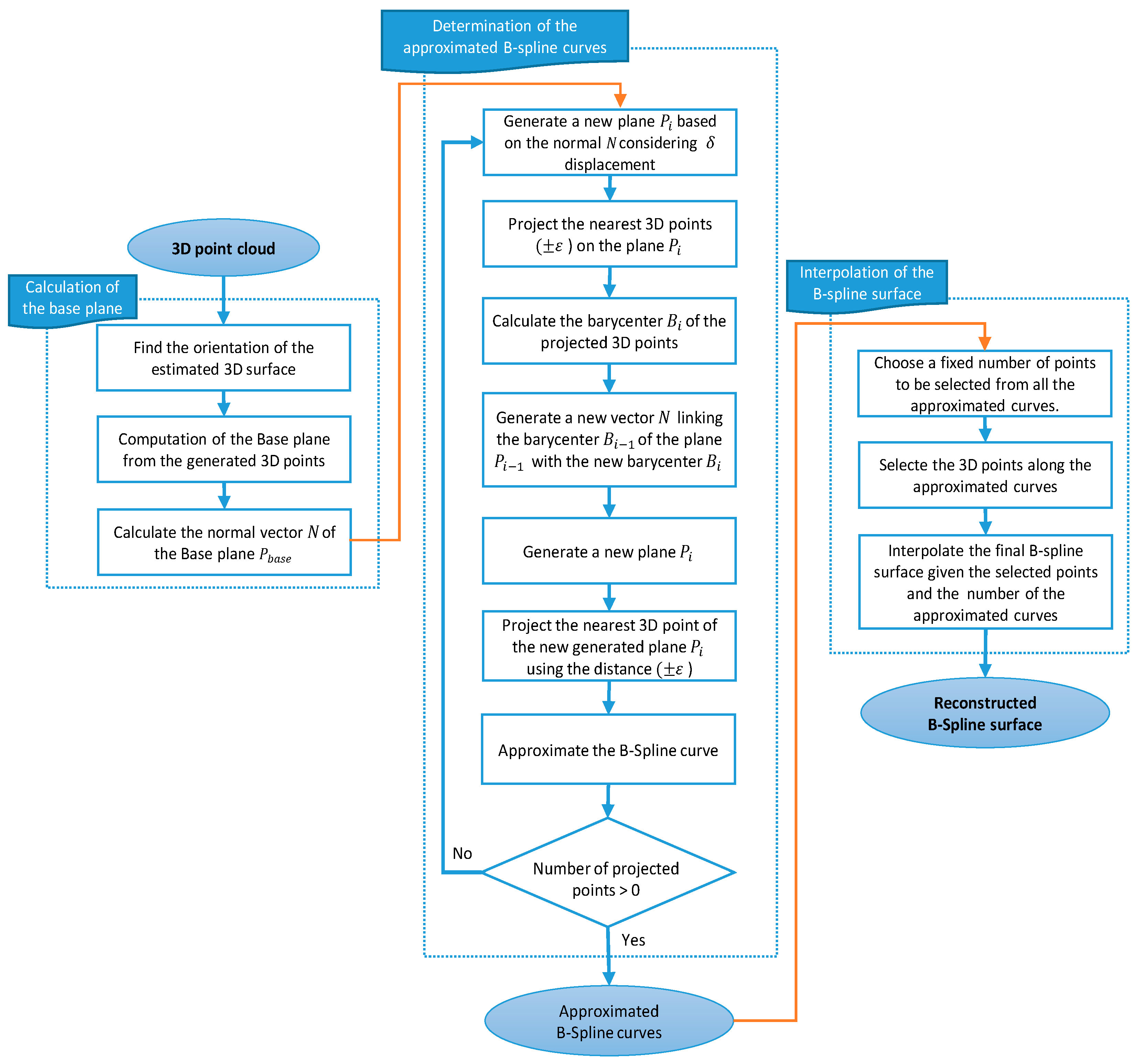
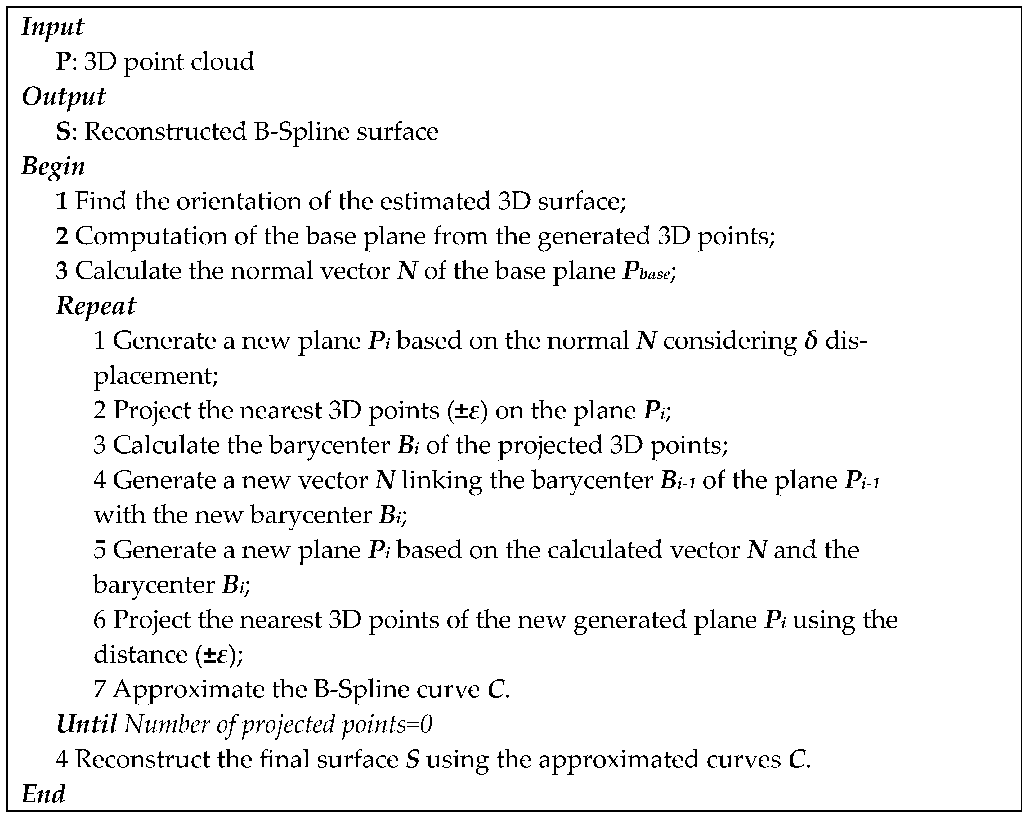
3. Proposed Methodology

A well-fitting design requires an efficient process of CAD-model rebuilding of data acquired from the patient’s limb. The proposed approach to the design of a customized orthosis involves the reconstruction of the 3D surface from a point cloud. In fact, the main objective is to accurately reconstruct a B-Spline surface that should be reconstructed given a 3D point set acquired by a 3D laser scanner. Figure 1 presents an overview of the surface reconstruction process. This rebuilt surface is interpolated using approximated B-Spline curves, which is characterized by a fitting accuracy able to satisfy most reverse engineering requirements [23].
Figure 2 represents a flowchart of the overall approach. The general algorithm (Figure 3) consists of three general steps: calculate the base plane, determine the approximated B-Spline curves, and interpolate the B-Spline surface. In the following sub-sections, each step is detailed.

3.1. Calculation of the Base Plane

  • Determination of the orientation of the estimated 3D surface
Firstly, the orientation of the 3D surface is estimated using the inertia matrix of the input 3D points. Given a set of unorganized points P i = { ( x i , y i , z i ) } , for i = 1 , . . . , n , the coordinates of the centroid G of the input 3D points P i are given by Equation (1).
x G , y G , z G = 1 n i = 0 n x i i = 0 n y i i = 0 n z i
Given the calculated center of gravity, the inertia matrix is defined by Equation (2), such that M i j i , j = 1   to   3 is defined by Equations (2)–(8).
M G = M 11 M 12 M 13 M 21 M 22 M 23 M 31 M 32 M 33
Such that
M 11 = i = 0 n 1 x G x i 2 n
M 22 = i = 0 n 1 y G y i 2 n
M 33 = i = 0 n 1 z G z i 2 n
M 12 = M 21 = i = 0 n 1 x G x i y G y i n
M 13 = M 31 = i = 0 n 1 x G x i z G z i n
M 23 = M 32 = i = 0 n 1 y G y i z G z i n
the inertia matrix M G is diagonalizable since it is a real symmetric positive-definite matrix. Thus, eigenvectors of the M G define the three inertia axes ( V 1 , V 2 , V 3 ) of the system formed by the set of points P i . The eigenvector associated with the largest eigenvalue is assumed as the inertia axis V 3 . The axis passing through the point G along the inertia axis V 3 determines the orientation of the 3D object.
  • Determination of the base plane
This step consists of finding three distinct points P m i n i (i = 1 to 3) which allow the definition of the equation of the base plane in R 3 . To find the first point P m i n 1 , each input point P i is projected on the inertia axis V 3 and its V 3 -coordinate (the coordinate of the point with respect to the V 3 inertia axis) is computed. The point P m i n 1 corresponds to the smallest V 3 -coordinate. Now, let P m i n 1 denote the orthogonal projection of the point P m i n 1 on the inertia axis V 3 , and P p r o j stands for the orthogonal projection of P i on the plane defined by the three points G , P m i n 1 , and P m i n 1 . Moreover, angles defined by the two lines ( P m i n 1 P m i n 1 ) and ( P m i n 1 Pproj) should be computed. Therefore, the point P p r o j corresponding to the smallest angle defines the point P m i n 2 . Finally, P m i n 2 is considered a fixed point and, again, the smallest angle is identified to find the point P m i n 3 . The base plane is uniquely defined by the three points P m i n i (Figure 4).
The coefficients of the plane equation are calculated using Equation (9), where x i , y i , z i , i = 1   to   3 are the coordinates of the three points P m i n i . Given the calculated base plane, the normal vector N is determined using the cross product.
a x 1 + b y 1 + c z 1 = d a x 2 + b y 2 + c z 2 = d a x 3 + b y 3 + c z 3 = d
The determination of the base plane is critical for aligning the acquired data, removing noise, guiding surface reconstruction, and providing visual context in the 3D model reconstruction process from a 3D point cloud. By determining the base plane, the point cloud can be aligned with a known coordinate system, making it easier to integrate the point cloud data with other spatial information or models. The base plane provides information about the orientation and scale of the point cloud data. By defining a horizontal surface as the base plane, the orientation of the point cloud can be determined with respect to the ground or any other reference plane. This knowledge is important for accurate visualization, analysis, and measurements within the 3D model. The base plane can be used as a filtering or segmentation criterion to separate the point cloud data into meaningful subsets. By removing or isolating points that do not belong to the base plane, such as outliers or noise, you can improve the quality and reliability of the reconstructed 3D model. The base plane provides a starting point for surface reconstruction algorithms. By leveraging the known geometry of the base plane, such as planar fitting techniques, the reconstructed 3D model can be determined with higher accuracy. The base plane serves as a visual reference for the reconstructed 3D model. It helps users understand the orientation, spatial relationships, and context of the point cloud data. This information is particularly important when visualizing and interpreting the model for applications such as architecture, urban planning, or virtual reality.

3.2. Determination of the Approximated B-Spline Curves

This step aims to approximate a set of B-Spline curves to be used in the surface reconstruction. Given the normal vector N of the base plane, a plane F i is generated considering the δ -displacement value. Then, the nearest 3D points to F i considering the ( ± ε ) distance are projected on the generated plane F i . From these projected points, a barycenter B i is calculated to generate a vector N i + 1 linking this barycenter B i with the barycenter B i 1 . A new plane F i + 1 is generated based on the calculated vector N i + 1 and the barycenter B i (Figure 5). Next, the nearest 3D points to the newly generated plane F i + 1 are projected on this plane considering the distance ( ± ε ) . From these projected points, a B-Spline curve is approximated. This process is repeated until there are no more points to project on the last generated plane. The generation of the projected planes in the 3D surface reconstruction process are necessary for planar fitting, surface segmentation, surface reconstruction, and geometric representation. These planes provide valuable information and serve as a foundation for further processing and refinement in the reconstruction pipeline.
  • B-Spline curve approximation
The B-Spline curve approximation is a crucial step in the process of 3D surface reconstruction for achieving smoothness, noise reduction, surface regularization, parameterization, interpolation, extrapolation, and data compression. It enhances the quality and accuracy of the reconstructed surface, enabling various analysis and manipulation techniques in subsequent stages.
The B-Spline curve C is defined by Equation (10), given a set of input data points I _ i   ( i = 0   to   n ) , a degree p , and a number h ( n > h p 1 ) . The B-Spline curve of the degree p defined by ( h + 1 ) control points ξ _ i   ( i = 0   t o   h ) should be reconstructed according two conditions: The curve passes through the first and last data points, i.e., I 0 = C ( 0 ) = ξ 0 and I n = C ( 1 ) = ξ n , and the 3D data points are approximated by solving the least-squares problem.
C u = i = 0 h N i , p ( u ) ξ i
The equation of the curve approximation is defined by the relation (11).
C u = N 0 , p u ξ 0 + i = 1 h 1 N i , p u ξ i + N h , p ( u ) ξ h
Least squares is the optimal solution to approximate this curve. The sum of all squared error distances is defined by Equation (12). Equation (12) can be written as in (13).
f ξ 1 , , ξ h 1 = k = 1 h 1 I k C ( t k ) 2
f ξ 1 , , ξ h 1 = k = 1 h 1 Q k i = 1 h 1 N i , p t ξ i 2 ; s u c h   a s   Q k = I k N 0 , p ( u ) ξ 0 N h , p ( u ) ξ h
The Levenberg–Marquardt algorithm is applied to solve the approximation problem. The algorithm requires the initialization of the degree of the B-Spline curve and the control points ξ i to be optimized. Then, the system of linear equations for ξ i is solved to find the best control points that approximate the curve. At each iteration of the algorithm, 5892 new control points are calculated until the distance between the points of the B-Spline curve defined by these control points and the set of 3D points is minimized (Figure 6).

3.3. Interpolation of the B-Spline Surface

The B-Spline curve/surface interpolation or approximation technique excels in representing a small number of data points as a smooth curve or surface. Its ability to smooth out irregularities, flexibility in shape control, interpolation and approximation capabilities, data reduction advantages, and high continuity make it a powerful tool for accurately and efficiently representing data with minimal points. The advantage of B-Spline curve/surface interpolation or approximation is its ability to represent a small number of data points as a smooth curve or surface. This property is particularly valuable in situations where the available data points are sparse or unevenly distributed.
Based on the reconstructed curves, an algorithm is developed to reconstruct the final B-Spline surface. This surface is defined on each point by Equation (14) [24].
S u , v = i = 0 n j = 0 m β i , p ( u ) β j , q ( v ) ξ i , j
The knot vectors U and V have ( r + 1 ) and ( s + 1 ) nodes, respectively, where r = n + p + 1 and s = m + q + 1 . ξ i , j are the surface control points. This surface is defined with a p degree in the u -direction and a q degree in the v -direction, such that u and v are the location parameters that locate a point in the surface [15]. The surface node values must be in the interval [0, 1]. Thus, the knot vectors should take the form in Equation (15).
S u , v = i = 0 n j = 0 m β i , p ( u ) β j , q ( v ) ξ i , j
β i , p and β j , q are the B-Spline basis functions of the p degree in the u -direction and the q degree in the v -direction. These basis functions are computed in a recursive way (16).
β i , p u = u u i u i + p u i . β i , p 1 u + u i + p + 1 u u i + p + 1 u i + 1 . β i + p + 1 , p 1 u s u c h   a s N i , 0 u = 1   i f   u i u u i + 1 E l s e   N i , 0 u = 0
The interpolation of the B-Spline surface requires the following steps:
  • Choose a fixed number α of points to be selected from all the reconstructed curves.
  • Generate a perpendicular plane F p to the base plane.
  • Given the barycenter of each approximated curve, the plane F p is rotated using a calculated angle α based on the number α of selected points.
  • The selected points on each curve are obtained by the intersection of the rotated plane with the corresponding B-Spline curve.
  • Interpolate the final B-Spline surface given all the selected points and the number of approximated curves.

4. Experimental Results on Quality Assessment

The quality of the reconstructed surface can be influenced by the characteristics of the point cloud obtained from the scan. Point clouds may exhibit various characteristics such as noise, outliers, irregularities, or missing data, which can affect the reconstruction process. These factors can affect the quality and the need for cleaning or smoothing operations. These operations help to improve the quality and reliability of the reconstructed surface by reducing noise, eliminating outliers, addressing irregularities, and filling in missing data. Cleaning and smoothing the point cloud enable the reconstruction algorithm to work with a more accurate and consistent dataset, resulting in a higher-quality reconstructed surface. These pretreatment operations are applied on the given 3D point cloud before executing the proposed approach.
The robustness of the developed algorithm is evaluated based on the reconstruction error of two input data point sets. The Maximum Root Mean Square Error (MRMS) metric is used to evaluate the surface reconstruction quality. The MRMS metric calculates the distance between the points of the initial surface S and the reconstructed surface S (17) [25].
M R M S = m a x ( d R M S ( S , S ) , d R M S ( S , S ) )
d R M S represents the root mean square error between two surfaces S and S (18).
d R M S S , S = 1 n ( x 2 + y 2 + z 2 )
where x , y and z are the normal distances between two points p and p along the surfaces S and S in the x -, y -, and z -directions, and n is the total number of points.
The reconstruction cases consist of two data clouds containing 6294 and 6365 points, respectively. Figure 7 presents the reconstruction results using the proposed method. The MRMS errors of the two reconstructed surfaces are mentioned in (Table 2). The reconstruction quality is acceptable as compared to the 700 × 10−6 mm root mean square error resulting from the reconstruction of regular feature models in [26].
The proposed approach can be used in various fields and industries such as Computer Vision and Robotics, Virtual Reality and Augmented Reality, Cultural Heritage and Archaeology, Medical Imaging and Biomechanics, Industrial Design and Manufacturing, and Architecture and Construction. In this paper, we have applied the developed approach in order to reconstruct a customized orthosis for human parts (finger and foot).

5. Surface Reconstruction Results

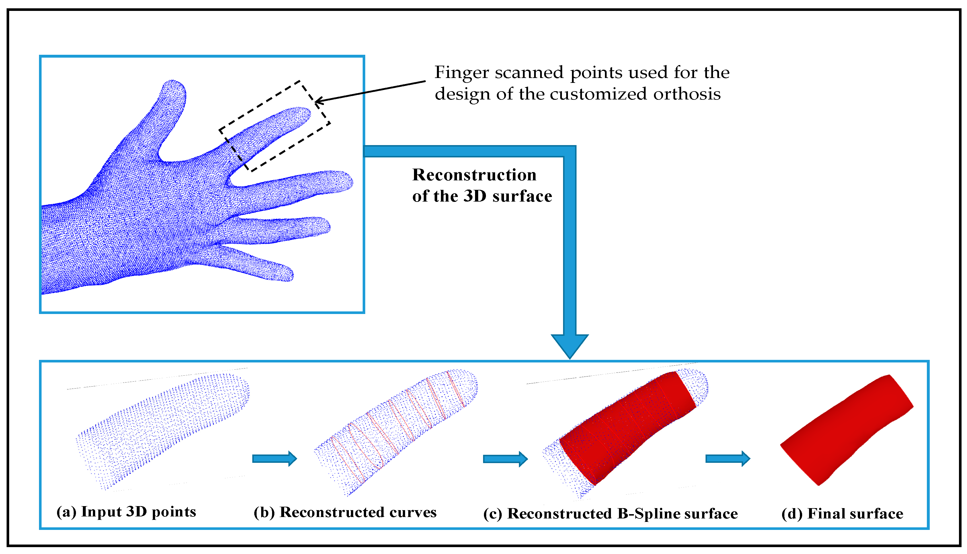
5.1. Surface Reconstruction for Customized Finger Orthosis Design

In the design process of an orthotic model for a specific human finger, the body part is first 3D-scanned (Figure 8). Then, the proposed algorithm is executed to reconstruct the corresponding B-Spline surface. The resulting MRMS error is 6.418 × 10⁻⁷ mm. Using the same input data, the surface is reconstructed using Ben Makhlouf’s method [22]. An MRMS error of 1.006 × 10⁻⁶ mm is obtained.
The result demonstrates that the reconstruction error using the proposed approach is lower than the reconstruction error resulting from the method in [22]. In this paper, the Levenberg–Marquardt algorithm is developed to approximate the B-Spline surface with a minimum error. In the proposed approach, those errors are minimized since the approximation is established in the curve generation level, the approximation accuracy is driven by the reference plan number (i.e., δ -displacement value), and the B-Spline surface is generated by the interpolation method.
This comparison study proves the efficiency and robustness of the developed approach. These results bridge the research gap of surface reconstruction inefficiency for rapid prototyping of orthoses.

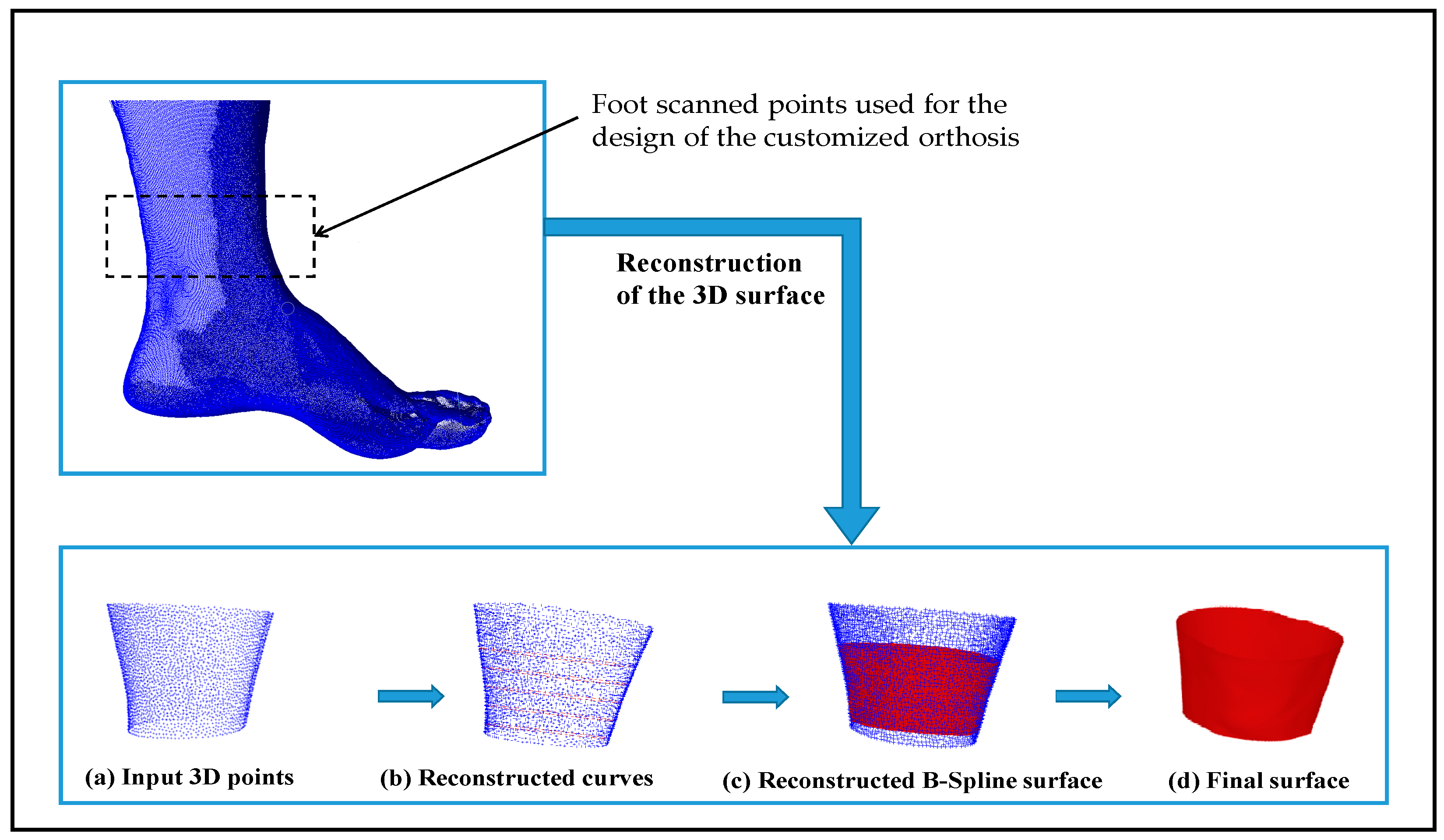
5.2. Surface Reconstruction for Customized Orthosis Design of Part of Foot

In this case, study, a customized orthotic model for a part of a human foot is reconstructed given a 3D set of points obtained from a 3D scanner (Figure 9). The developed algorithm is executed to reconstruct the adequate B-Spline surface of the human foot part. The measured MRMS error is 9.53 × 10⁻⁶ mm. The reconstruction error of the same input surface using Ben Makhlouf’s method [22] is 2.43 × 10⁻⁵ mm.
This second case study proves that the proposed approach improves the reconstruction quality and guarantees more precision of the customized orthotic model.

5.3. Discussion

The obtained results prove that the proposed methodology is efficient and can help clinical staff to model an adequate orthosis for a specific patient by simply scanning the patient’s body part. The developed algorithm gives a precise reconstruction of the 3D surface compared to existing methods. In fact, it is true that the precise reconstruction of the 3D surface affects the quality of the orthotic model, but adaptive support with the elastic deformity of the soft tissue can also affect the quality of the final product. In future work, new criteria should be considered to validate the methodology. In addition, an automatic definition of the plane displacement according to the input points’ size will optimize the method’s accuracy and runtime. Further experimental investigations including AM of orthopedic devices and rehabilitation treatment analysis will prove the above verdict.

6. Conclusions

This paper presents an original approach based on the B-Spline curve approximation for reconstructing a 3D surface. Several steps are followed to obtain an accurate reconstructed surface. First, the orientation of the surface to be reconstructed is determined, allowing the association of a base plane with the input point set. Then, reference planes are created in an iterative process based on a user-predefined displacement. In each iteration, the nearest points to the reference plane are projected to approximate the B-Spline curve. By the approximation of selected points on the reconstructed curves, the final B-Spline surface is determined. Two modeled surfaces and two scanned parts of the human body are reconstructed to evaluate the proposed approach. Numerical experiments highlight the reconstructed surface quality. Also, the experiments show the suitability and reliability of the proposed method for customized orthosis designs. This efficient technique is a promising tool for enhancing the patient’s comfort.

Author Contributions

Conceptualization, N.H.A. and B.L.; methodology, N.H.A., A.B.M. and B.L.; software, A.B.M. and B.L.; validation, N.H.A., A.B.M. and B.L.; formal analysis, N.H.A., A.B.M. and B.L.; investigation, N.H.A., A.B.M., B.L. and M.T.; resources, A.B.M. and B.L.; data curation, A.B.M. and B.L.; writing—original draft preparation, N.H.A., A.B.M., B.L., M.T. and K.H.; writing—review and editing, N.H.A., A.B.M., B.L., M.T. and K.H.; visualization, N.H.A., A.B.M. and B.L.; supervision, B.L.; project administration, B.L. All authors have read and agreed to the published version of the manuscript.

Funding

The authors extend their appreciation to the Deanship of Scientific Research, Imam Mohammad Ibn Saud Islamic University (IMSIU), Saudi Arabia, for funding this research work through Grant No. (221414010).

Institutional Review Board Statement

Not applicable.

Data Availability Statement

The raw data supporting the conclusions of this article will be made available by the authors on request.

Conflicts of Interest

The authors declare no conflict of interest.

References

  1. Disability and Health. Available online: https://www.who.int/news-room/fact-sheets/detail/disability-and-health (accessed on 15 November 2022).
  2. Stein, R.B.; Everaert, D.G.; Thompson, A.K.; Chong, S.L.; Whittaker, M.; Robertson, J.; Kuether, G. Long-Term Therapeutic and Orthotic Effects of a Foot Drop Stimulator on Walking Performance in Progressive and Nonprogressive Neurological Disorders. Neurorehabilit. Neural Repair 2010, 24, 152–167. [Google Scholar] [CrossRef] [PubMed]
  3. Mavroidis, C.; Ranky, R.G.; Sivak, M.L.; Patritti, B.L.; DiPisa, J.; Caddle, A.; Gilhooly, K.; Govoni, L.; Sivak, S.; Lancia, M.; et al. Patient Specific Ankle-Foot Orthoses Using Rapid Prototyping. J. Neuroeng. Rehabil. 2011, 8, 1–11. [Google Scholar] [CrossRef] [PubMed]
  4. Fitzpatrick, A.P.; Mohanned, M.I.; Collins, P.K.; Gibson, I. Design of a Patient Specific, 3D Printed Arm Cast. In Proceedings of the International Conference on Design and Technology, Geelong, Australia, 5–8 December 2016. [Google Scholar] [CrossRef]
  5. Blaya, F.; Pedro, P.S.; Pedro, A.B.S.; Lopez-Silva, J.; Juanes, J.A.; D’amato, R. Design of a Functional Splint for Rehabilitation of Achilles Tendon Injury Using Advanced Manufacturing (AM) Techniques. Implementation Study. J. Med. Syst. 2019, 43, 122. [Google Scholar] [CrossRef] [PubMed]
  6. Popescu, D.; Zapciu, A.; Tarba, C.; Laptoiu, D. Fast Production of Customized Three-Dimensional-Printed Hand Splints. Rapid Prototyp. J. 2020, 26, 134–144. [Google Scholar] [CrossRef]
  7. Commean, P.K.; Smith, K.E.; Vannier, M.W. Design of a 3-D Surface Scanner for Lower Limb Prosthetics: A Technical Note. J. Rehabil. Res. Dev. 1996, 33, 267–278. [Google Scholar] [PubMed]
  8. Palousek, D.; Rosicky, J.; Koutny, D.; Stoklásek, P.; Navrat, T. Pilot Study of the Wrist Orthosis Design Process. Rapid Prototyp. J. 2014, 20, 27–32. [Google Scholar] [CrossRef]
  9. Choi, W.S.; Jang, W.H.; Kim, J.B. A Pilot Study for Usefulness of Customized Wrist Splint By Thermoforming Manufacture Method Using 3D Printing: Focusing on Comparative Study with 3D scanning Manufacture Method. J. Rehabil. Welf. Eng. Assist. Technol. 2018, 12, 149–158. [Google Scholar] [CrossRef]
  10. Mahmood, N.; Camallil, O.; Tardi, T. Multiviews Reconstruction for Prosthetic Design. Int. Arab. J. Inf. Technol. 2012, 9, 49–55. [Google Scholar]
  11. Venkateswaran, N.; Hans, W.J.; Padmapriya, N. 3D Design of Orthotic Casts and Braces in Medical Applications. Adv. Mater. Process. Technol. 2021, 7, 136–149. [Google Scholar] [CrossRef]
  12. Chaparro-Rico, B.D.M.; Martinello, K.; Fucile, S.; Cafolla, D. User-Tailored Orthosis Design for 3D Printing with Plactive: A Quick Methodology. Crystals 2021, 11, 561. [Google Scholar] [CrossRef]
  13. Hoppe, H.; DeRose, T.; Duchamp, T.; McDonald, J.; Stuetzle, W. Surface Reconstruction from Unorganized Points. Comput. Graph. (ACM) 1992, 26, 71–78. [Google Scholar] [CrossRef]
  14. Dinh, H.Q.; Turk, G.; Slabaugh, G. Reconstructing Surfaces Using Anisotropic Basis Functions. In Proceedings of the Eighth IEEE International Conference on Computer Vision. ICCV 2001, Vancouver, BC, Canada, 7–14 July 2001; IEEE: Piscataway, NJ, USA, 2001; Volume 2, pp. 606–613. [Google Scholar] [CrossRef]
  15. Carr, J.C.; Beatson, R.K.; Cherrie, J.B.; Mitchell, T.J.; Fright, W.R.; McCallum, B.C.; Evans, T.R. Reconstruction and Representation of 3D Objects with Radial Basis Functions. In Proceedings of the 28th Annual Conference on Computer Graphics and Interactive Techniques-SIGGRAPH ’01, Los Angeles, CA, USA, 12–17 August 2001; ACM Press: New York, NY, USA, 2001; pp. 67–76. [Google Scholar] [CrossRef]
  16. Hornung, A.; Leif, K. Robust Reconstruction of Watertight 3D Models from Non-Uniformly Sampled Point Clouds without Normal Information. In Eurographics Symposium on Geometry Processing; Konrad, P., Alla, S., Eds.; The Eurographics Association: Sardinia, Italy, 2006; pp. 41–50. [Google Scholar] [CrossRef]
  17. Alliez, P.; David, C.-S.; Tong, Y.; Desbrun, M. Voronoi-Based Variational Reconstruction of Unoriented Point Sets. In Symposium on Geometry Processing; Belyaev, A., Garland, M., Eds.; The Eurographics Association: Barcelona, Spain, 2007; Volume 67, pp. 39–48. [Google Scholar] [CrossRef]
  18. Huang, H.; Li, D.; Zhang, H.; Ascher, U.; Cohen-Or, D. Consolidation of Unorganized Point Clouds for Surface Reconstruction. ACM Trans. Graph. 2009, 28, 1–7. [Google Scholar] [CrossRef]
  19. Rouhani, M.; Sappa, A.D.; Boyer, E. Implicit B-Spline Surface Reconstruction. IEEE Trans. Image Process. 2015, 24, 22–32. [Google Scholar] [CrossRef] [PubMed]
  20. Louhichi, B.; Nizar, A.; Mounir, H.; Abdelmajid, B.; Vincent, F. An Optimization-based Computational Method for Surface Fitting to Update the Geometric Information of An Existing B-Rep CAD Model. Int. J. CAD/CAM 2010, 9, 17–24. [Google Scholar]
  21. Louhichi, B.; Abenhaim, G.N.; Tahan, A.S. CAD/CAE Integration: Updating the CAD Model after a FEM Analysis. Int. J. Adv. Manuf. Technol. 2014, 76, 391–400. [Google Scholar] [CrossRef]
  22. Ben Makhlouf, A.; Louhichi, B.; Mahjoub, M.A.; Deneux, D. Reconstruction of a CAD Model from the Deformed Mesh Using B-Spline Surfaces. Int. J. Comput. Integr. Manuf. 2019, 32, 669–681. [Google Scholar] [CrossRef]
  23. Wang, T.-R.; Liu, N.; Yuan, L.; Wang, K.-X.; Sheng, X.-J. Iterative Least Square Optimization for the Weights of NURBS Curve. Math. Probl. Eng. 2022, 2022, 1–12. [Google Scholar] [CrossRef]
  24. Piegl, L.; Tiller, W. The NURBS Book, 1st ed.; Monographs in Visual Communications; Springer: Berlin/Heidelberg, Germany, 1995. [Google Scholar] [CrossRef]
  25. Niu, Y.; Zhong, Y.; Guo, W.; Shi, Y.; Chen, P. 2D and 3D Image Quality Assessment: A Survey of Metrics and Challenges. IEEE Access 2018, 7, 782–801. [Google Scholar] [CrossRef]
  26. Li, F.; Longstaff, A.P.; Fletcher, S.; Myers, A. Rapid and Accurate Reverse Engineering of Geometry Based on a Multi-Sensor System. Int. J. Adv. Manuf. Technol. 2014, 74, 369–382. [Google Scholar] [CrossRef]
Figure 1. Surface reconstruction process.
Prosthesis 06 00008 g001
Figure 2. Proposed approach flowchart.
Prosthesis 06 00008 g002
Figure 3. Algorithm of B-Spline surface reconstruction.
Prosthesis 06 00008 g003
Figure 4. Base plane generation.
Prosthesis 06 00008 g004
Figure 5. Iterative plane generation.
Prosthesis 06 00008 g005
Figure 6. B-Spline curve approximation: (a) Approximation points, (b) Reconstructed curve.
Prosthesis 06 00008 g006
Figure 7. The surface reconstruction (a) 1st case, (b) 2nd case.
Prosthesis 06 00008 g007
Figure 8. Surface reconstruction steps for finger orthosis design.
Prosthesis 06 00008 g008
Figure 9. Surface reconstruction steps for foot orthosis design.
Prosthesis 06 00008 g009
Table 1. Comparison of 3D limb reconstruction methods: differences and limitations.
MethodDifferencesLimitations
Hoppe et al. [13]Approximated 3D surface reconstruction from unorganized 3D point cloudNeed for improvement in method accuracy
Commean et al. [7]Multiple camera setup for simultaneous capture of the lower limbComplex process and difficult to achieve high accuracy
Dinh et al. [14]Surface reconstruction technique based on tensor field-driven anisotropic basis functionsCaptures sharp features, no need for prior knowledge about surface topology, moderate accuracy (average Euclidean distance error of 0.0120)
Carr et al. [15]Surface reconstruction using radial basis functions (RBF) and hole-fillingEfficient and accurate reconstruction, especially for large datasets
Hornung and Kobbelt [16]Unsigned distance function-based surface reconstruction with resilience to noiseReconstruction without normal information, resilience to misalignment noise
Alliez et al. [17]Voronoi algorithm-based surface reconstruction using surface normal computationSurface normal and tensor field computation using Voronoi diagram
Huang et al. [18]Weighted locally optimal projection and principal component analysis for surface reconstructionDenoising of input 3D point cloud, normal estimation, priority-guided normal propagation, moderate accuracy
Mahmood et al. [10]Surface reconstruction from video image data using a pinhole cameraComplex process based on video frames, challenging to achieve high accuracy
Rouhani et al. [19]Implicit B-Spline surface-based reconstruction algorithmNo parameterization required, solving a system of linear equations
Louhichi et al. [21]Weighted displacement estimation-based surface reconstruction for deformed meshImproved algorithm for control point approximation in B-Spline surface reconstruction, comparison of error with existing methods
Makhlouf et al. [22]Enhanced weighted displacement estimation-based surface reconstruction algorithm for deformed meshImproved control point approximation in B-Spline surface reconstruction, comparison with existing methods for efficiency validation
Venkateswaran et al. [11]Microsoft Kinect sensor-based 3D reconstruction method using RGB and depth imagesSignificant reconstruction errors
Chaparro-Rico et al. [12]3D scan of the limb using MATLAB software, boundary surface generation using SolidWorks softwareAccuracy not specified
OverallOngoing improvement in the quality of resulting surfacesCurrent methods need further progress in result robustness and accuracy to meet medical device design requirements
Table 2. Reconstruction error.
Number of PointsReconstruction Error (mm)
1st case62940.06821 × 10−6
2nd case63653.204 × 10−6
Disclaimer/Publisher’s Note: The statements, opinions and data contained in all publications are solely those of the individual author(s) and contributor(s) and not of MDPI and/or the editor(s). MDPI and/or the editor(s) disclaim responsibility for any injury to people or property resulting from any ideas, methods, instructions or products referred to in the content.

