Progress in Developing an Emulation of a Neuromorphic Device That Is Predicted to Enhance Existing Cortical Prosthetic Vision Technology by Engaging Desired Visual Geometries

Abstract

The utility of currently available cortical prosthetic vision systems is disappointing. The essential features of a neuromorphic device that is predicted to enhance vision provided by available systems follow from a hypothesis which states that the objective and subjective aspects of cortical prosthetic vision jointly constitute patterns that emerge from specified synaptic interactions. The research reported here completes several required steps in developing an emulation of this device: (1) replication of small-scale simulations that are consistent with the hypothesis using the NEST (Écublens, Vaud, Switzerland) simulator, which can also be used for full-scale network emulation by a neuromorphic computer; (2) testing whether results consistent with the hypothesis survive increasing the scale and duration of simulations; (3) establishing a method that uses numbers of spikes produced by network neurons to report the number of phosphenes produced by cortical stimulation; and (4) simulating essential functions of a neuromorphic device which is predicted to enhance current prosthetic systems. NEST simulations replicated early results and increasing their scale and duration produced results consistent with the hypothesis. A decision function created using multinomial logistic regression correctly reported the expected number of phosphenes for three sets of 2080 spike number distributions in which half of each set arises from simulations expected to yield continuous visual forms by engaging a desired visual geometry. A process for modulating electrical stimulation amplitude based on intermittent population recordings that is predicted to produce desired visual geometries was successfully simulated. Implications of these results for future research are discussed.

1. Introduction

Since the earliest demonstration of a very crude cortical prosthesis in 1958 [1], researchers have made efforts to produce a useful cortical prosthetic vision (CPV) system that would help to improve the lives of the large and increasing population of blind individuals [2,3]. Comparing the presently available CPV technology with what was available in the 1960’s and 1970’s reveals tremendous improvements in every technical area [4,5]. Furthermore, long-term research and development programs which capitalize on cutting-edge imaging, neural recording, and neural stimulation technologies hold the promise of delivering prosthetic vision systems that provide visual experiences with much greater detail than is possible with existing systems [6].

Despite this progress, the quality of vision that is provided by current systems is very poor, and this is not simply the result of a lack of visual detail. The mechanisms through which neural systems produce normal vision, including those in primary visual cortex (V1), the target of electrical stimulation in CPV, are poorly understood [7,8]. It is undoubtedly true that the rudimentary vision provided by the most technically sophisticated CPV systems that are available is in part the result of our poor understanding, and I think that developing the understanding that is needed to produce useful vision requires dealing with a problem that has not even been mentioned in CPV publications.

Normal vision and CPV have both objective neural aspects and subjective experiential aspects, and achieving a scientific understanding of how vision works involves grasping the physical significance of relationships between them. Developing such an understanding for experience in general has been called the “hard problem” by Chalmers [9,10]. A variety of general theories of conscious experience have been put forward subsequent to Chalmers’ now famous description [11], but they are not helpful in understanding the particular case of relationships between neural interactions in visual cortex and the specific experiences that are reported by individuals with CPV implants.

I will argue that the quality of visual experience and guidance of behavior that are produced by current CPV technology might be improved substantially if the subjective and objective aspects of CPV were both treated as physical phenomena, and if research was based on a hypothesis that specifically addresses the physical significance of relationships between them. The remainder of this section begins with a brief overview of CPV. Quantitative models of the subjective aspects of CPV which can be related to objective quantities included in neural network models are then described. This is followed by the introduction of a specific hypothesis regarding the nature of relationships between objective and subjective aspects of CPV and consideration of how the subjective aspects might be altered using presently available CPV technology. This section ends with a discussion of the specific aims of the computer simulation research that is reported in this paper.

1.1. CPV Systems Provide a Distribution of Phosphenes in Visual Space

In current CPV systems, video images captured by a camera mounted in eyeglasses or in goggles are used by a microprocessor to control delivery of electric current that stimulates neurons in V1 [12,13,14,15], which is the primary cortical target of input from the retinas (e.g., [16]). Neural networks that identify the opponent-color wavelength components of light, the orientation and movement of contrast, and the disparities between the regions of the two retinas on which an object forms an image are organized into the columns of V1 (e.g., [8,16]). Stimulation current likely induces additional spikes at various sites on the axons of neurons across cell types and layers of the cortex [17,18], and therefore likely affects networks involved in different aspects of visual processing. Cortical columns containing neural networks that represent the foveae and immediately surrounding central portions of the retinas and which provide color and high acuity vision are found in the most posterior region of V1, and the columns traversed as one moves anteriorly over V1 represent increasingly peripheral or eccentric portions of the retinas [16,19].

Stimulating V1 produces experiences that are quite different from the goal of producing a recognizable visual object. Above-threshold current delivered through a single electrode produces the experience of a typically achromatic bright spot called a phosphene, and simultaneous delivery of current through multiple electrodes produces multiple distinct phosphenes [16,20,21,22,23,24,25,26]. Phosphenes are described by individuals receiving electrical stimulation as existing in the environment, and the locations of phosphenes relative to the direction of gaze are determined by placement of electrodes on V1 relative to the representation of the foveae [20,27]. Consequently, a contrast-based event sensor [28] which detects the edges of an object can be used to choose electrodes that carry stimulation current, but the dependence of phosphene location on electrode placement implies that phosphenes will not appear at visual positions which closely match the shape of the object.

The dependence of phosphene position on the direction of gaze also implies that eye movements must alter the perceived locations of phosphenes. Brain stimulation studies corroborate this expectation [23,26,29], and a recent study of two patients with longstanding blindness and implanted with chronic neurostimulator devices provides details of how eye movements affect phosphene perception [30]. Caspi et al. [30] found a strong dependence of the visual locations of phosphenes on eye position at the time of stimulation but not at a later time of pointing to perceived phosphene locations. This result has clear implications for how eye scanning should be integrated with stimulation. The authors suggest that patients with V1 implants might be trained to use head movements to shift the field-of-view and to use eye movements to alter the visual field of each stimulating electrode, much as patients with retinal prostheses were trained to use head movements to shift the field-of-view of a camera and eye movements to shift regions of interest within the field-of-view [31].

Phosphene size grows up to a saturation point with the magnitude of stimulating current [32], but also with its visual eccentricity [20,33]. The latter effect is expected from the V1 magnification factor [16] which describes quantitatively how the size of the retinal region represented by neurons in a column of V1 increases with distance from the cortical representation of the fovea. The dependence of phosphene size on visual eccentricity places another constraint on the ability of CPV systems to produce recognizable visual forms.

The perception of continuous visual forms rather than discrete phosphenes has been reported in only one publication. A recent investigation [22] reported that sequentially stimulating electrodes along a path describing a visual form (letter) led to reported experiences of that form rather than of discrete phosphenes, and improved recognition dramatically. It was suggested that this technique, called current steering, may produce continuous forms via the activation of visual motion circuits. This intriguing finding raises the important questions of how activity in visual motion networks affects network activity directly involved in perception, and of why these effects produce this change in perception. Quantitative models of vision produced by CPV will be used to describe a hypothesis which suggests answers to these questions.

1.2. Models of Phosphenes and the Visual Geometry That They Occupy

Having quantitative models of phosphenes and visual space is helpful in thinking about how they are related to neural quantities and the kind of manipulations that might improve the quality of vision that is provided by current CPV technology. As shown below, these models also make it possible to simulate subjective aspects of CPV as well as objective neural activity. The visual space that phosphenes inhabit can be modeled as a visual geometry using relations between idealized, flattened V1 coordinates $\left(x,y\right)$ and retinal eccentricity ${\epsilon }_r$ and azimuth $a_r$ coordinates (e.g., [19,34], Ch. 2),

$$x=\gamma \ln \left(1+{\epsilon }_{\mathrm{r}}/{\epsilon }_0\right), y=-\gamma {\epsilon }_r\pi a_r/\left({\epsilon }_0+{\epsilon }_r\right){180}^{°}$$

(1)

and then approximating visual geometry coordinates $\widehat{\epsilon }$ and $\widehat{a}$ by finding the inverse of Equation (1),

$$\begin{gathered} \widehat{\epsilon }={\epsilon }_0\left[exp\left(x/\gamma \right)-1\right], \\ \widehat{a}=-{180}^{°}y exp\left(x/\gamma \right)/\gamma \pi \left[exp\left(x/\gamma \right)-1\right]. \end{gathered}$$

(2)

As in [35,36], hats are used to decorate quantities that describe aspects of visual experience in order to distinguish them from objectively measurable quantities that describe aspects of neural networks, such as variables on which synaptic strengths depend. Values $\gamma =12 \mathrm{mm}$ and ${\epsilon }_0=1^{°}$ have been estimated from the macaque monkey [17] and are used in simulations.

An idealized flattened V1 geometry and a corresponding visual geometry created using Equations (1) and (2) are depicted in Figure 1. The V1 geometry is composed of 939 idealized cortical columns and the visual geometry of 939 corresponding visual regions. As in [35,36], the visual geometry was constructed by using Equation (2) to transform coordinates of the center of V1 column $i$ to values $\left({\widehat{\epsilon }}_i,{\widehat{a}}_i\right)$ of idealized visual geometry coordinates, assigning the value ${\left(0.15+0.09{\widehat{\epsilon }}_i\right)}^{1.2}$ to the radius of visual geometric region ${\widehat{R}}_i$, and then converting $\left({\widehat{\epsilon }}_i,{\widehat{a}}_i\right)$ values to cartesian coordinates $\left({\widehat{x}}_i^{°},{\widehat{y}}_i^{°}\right)$ that specify the center of each visual region in degrees of visual angle. It has been estimated that currents greater than $100 \mathsf{\mu }\mathrm{A}$ delivered through a microelectrode are likely to activate much of the volume of a V1 column [33], and the sizes of phosphenes that are generated using surface electrode stimulation suggest that neurons in one or more columns are activated [26]. It is therefore assumed that each phosphene inhabits at least one visual geometric region ${\widehat{R}}_i$.

Because it seems unlikely that the lightness of a phosphene can be modeled using a single real number, an interval of values is used [35,36]. It is assumed that Blue-Yellow and Red-Green opponent channel neurons are activated approximately equally by electrical stimulation, thereby resulting in typically achromatic phosphenes [4,20]. Idealized lightness values can then be modeled by a time-dependent lightness distribution

$$\widehat{l}\left({\widehat{x}}_i^{°},{\widehat{y}}_i^{°},t\right)=s_0{f}_L{\left(x_i,y_i,t\right)}^{l_0}.$$

(3)

In this equation, $f_L\left(x_i,y_i,t\right)$ is the frequency of spikes generated by a lightness channel neuron in V1 column $i$ with center coordinates $\left(x_i,y_i\right)$ at time $t.$ An idealized lightness interval distribution is mapped from the spike frequencies of a set of lightness channel neurons in each column. This can be done by supposing that there are multiple lightness channel neurons in each column, using Equation (3) to find the minimum and maximum lightness values that correspond to the minimum and maximum frequencies of action potentials generated by those neurons, and defining an interval that ranges from the minimum lightness value to the maximum lightness value.

1.3. A Hypothesis Regarding the Nature of Relationships between Objective and Subjective Aspects of CPV

The hypothesis which motivates the research that is described below states that both objective and subjective aspects of the visual geometry constitute a single self-organized pattern that arises from one system of synaptic interactions, and both objective and subjective aspects of the lightness interval distribution constitute a pattern that arises from a second system of interactions. Relationships between quantities that model subjective and objective features of the pattern are described as mappings that arise from the self-organization of the patterns, thereby asserting that subjective aspects play no causal role in altering objective aspects. Although this hypothesis is a pillar of the sense element engagement theory of CPV [35,36], its role here is limited to providing an explanation of how a neuromorphic device that is added to an existing CPV system might alter the perception of phosphenes.

The visual geometry pattern is presumed to result from interactions mediated by a geometric (G) system of synapses with strengths that are a mathematical function of an objective neural variable which has values that equal distances within and between regions in the visual geometry. Similarly, the lightness interval distribution pattern is presumed to result from interactions mediated by a lightness (L) system of synapses with strengths that are a function of an objective neural variable which has values that equal absolute differences in lightness within and between the lightness intervals on visual regions. The quantities ${\epsilon }_0$ and $\gamma$ in Equation (2) are viewed as order parameters that characterize the visual geometry pattern, and $s_0$ and $l_0$ in Equation (3) are viewed as order parameters that characterize the lightness interval distribution pattern (for information on order parameters see [37,38]). Equations (2) and (3) show that the visual geometry vanishes as ${\epsilon }_0\to 0$, the lightness interval distribution vanishes as $s_0\to 0$, and both patterns emerge as ${\epsilon }_0\to 1$ and $s_0\to 1$. As the patterns emerge, subjective distances within the visual geometry map to G system strengths and subjective differences in lightness within the lightness interval distribution map to L system strengths.

In the language of self-organized pattern formation, the changes in values of the two order parameters occur as the value of a control parameter approaches a critical value [37,38]. The control parameter for both the visual geometry and lightness interval distribution patterns is assumed to be the frequency of extrinsic spikes which have an excitatory effect on excitatory network neurons. If this is correct, then G and L system synapses within every column and between neighboring columns of the network become continuously active when a critical frequency of extrinsic excitatory spikes is reached. The visual geometry and lightness interval distribution patterns then emerge.

With the possible exception of modulation of G strengths by a change in vergence [16] which results in changes of perceived phosphene distance and size, it will be assumed that G strengths remain constant. In order for changes in the cortical columns that receive electrical stimulation above the threshold for producing a phosphene to produce a different subjective pattern of phosphenes, stimulation must alter L system strengths. It is presumed that changes in the frequencies of spikes produced by opponent-color channel neurons that result from changes in the stimulation pattern alter values of the neural variable that behaves like an absolute difference in lightness values, thereby mediating the change in L system strengths.

Computer simulations of neurons in a neural network spanning 25 of the columns represented by darker circles in Figure 1a and numbered 1–25 in Figure 2 have shown that the proportion of active excitatory neurons increases rapidly with the frequency of extrinsic spikes which have an excitatory effect on excitatory network neurons, and that excitatory neurons in all 25 columns become continuously active when the frequency of extrinsic spikes is above $60/\mathrm{s}$ [35,36]. These results were found both in the presence and absence of simulated electrical stimulation and are consistent with the contention that this frequency is a control parameter with a critical value of approximately $60/\mathrm{s}$.

1.4. How Desired Visual Geometries Might Be Engaged Using Available CPV Technology

As noted above, current steering was found to result in subjective reports of continuous forms and it was suggested that this effect results from activation of visual motion circuits [22]. If the sizes and shapes of visual regions result from the pattern of strengths of G system synaptic interactions, then appropriate changes in G system synaptic strengths can alter the shapes and sizes of regions in the visual geometry and thereby produce the experience of continuous visual forms. If this is correct, then visual motion circuits that are activated by current steering [22] alter G system synaptic strengths, as suggested in [35,36].

These considerations raise the question of whether introducing additional interactions between populations of network neurons would create a second visual geometry. Additional interactions might be mediated by a currently available CPV system that is used in conjunction with an external neuromorphic device. The simple block diagram shown in Figure 3 illustrates how the proposed mediation of interactions among populations of neurons in the cortical columns corresponding to visual regions 1, 4, 5, and 12 shown in Figure 2 could be added to a CPV system that employs 4 stimulation units.

The diagram is complete only for column 1 neurons to avoid unnecessary clutter. It is assumed that the electrodes for all 4 columns are alternately used for population recording and for stimulation on brief, alternating time intervals. During each recording interval, neuromorphic hardware is used to generate spikes when a threshold for the amplitude of population recordings from each column is exceeded. The neuromorphic spikes that are created using recordings from each (source) population activate neuromorphic current-based G system synapses of appropriate strengths for each (target) population that receives electrical stimulation, the synaptic currents modulate the membrane potential $V_m$ of a neuromorphic neuron that does not produce spikes, and values of the membrane potential are stored. When the recording interval ends, a stimulation interval of equal duration begins and the stored membrane potential values are used to modulate the amplitude of the current delivered by each stimulation unit. The mean stimulation current amplitude for each population is selected to be either below or above the threshold for producing a phosphene and each stimulation unit receives this value from the existing CPV system hardware.

It should be possible to introduce different extrinsically mediated visual geometries and therefore different visual forms by using different sets of neuromorphic G system synapses. For example, the device could be used to produce a visual geometry which yields continuous phosphenes at locations near the borders of an object that are inferred from the output of a contrast-sensitive event-based sensor [28] as described in Section 1.1. If a border fell along visual regions corresponding to columns 4 and 5, the neuromorphic synaptic strengths to populations of neurons in columns 1, 4, 5, and 12 could be made dependent on the visual distances that would arise if visual regions 4 and 5 were each made equal to the union of visual regions 1, 4, and 5 as they are depicted in Figure 2. Using a system based on these ideas with a human implant recipient would of course require estimation of the sizes, shapes, and positions of phosphenes in the visual field in order to estimate the sizes, shapes, and positions of the corresponding visual regions. The techniques reported in [30,32] appear to be very promising candidates for making the required estimations.

1.5. Aims of the Present Research

The present research completes several initial steps in following a neural network simulation and emulation strategy (initially proposed in [35,36]) to develop the neuromorphic device described above. A goal of this strategy is emulating a neural network that produces a full visual geometry as depicted in Figure 1b followed by emulation of a neuromorphic device that mediates G system interactions which are predicted to produce continuous visual forms. Emulations performed with a neuromorphic hardware system would produce information that would be very helpful in designing a neuromorphic device with the functions described in the previous section. The strategy also states that these emulations should be preceded by computer simulations of increasingly larger scale that would provide values of parameters required for the emulations. The BrainScaleS computer [39] has been identified as a neuromorphic hardware system that can be used for emulation of the neural network and neuromorphic device. This system uses the PyNEST interface [40] to the NEST software [41], and it was therefore decided that PyNEST and NEST should be employed for the required computer simulations.

The research that is reported here had the purpose of completing several steps in carrying out the requisite computer simulations. The first step is using the PyNEST interface and the NEST simulator to replicate the simulations of neurons in columns that correspond to visual regions numbered 1–25 in Figure 2 and reported in [35,36]. Those simulations were carried out in order to illustrate operation of the network with appropriate G system and L system synaptic strengths, and to determine if the frequency of extrinsic spikes that excite the excitatory neurons of the network acts as a control parameter for emergence of the visual geometry and lightness interval distribution patterns. There are differences in details of the models that are employed in the original Mathematica simulation code and those employed by NEST, and these differences are likely to produce some quantitative differences in results. However, it seems reasonable to demand that the qualitative behavior of the proposed neural network should be robust to such differences. In addition, the Mathematica simulation code used in the initial simulations had the primary purpose of producing extremely accurate estimates of synaptic conductance values, membrane potentials, and spike times without regard for the computational cost and duration of simulations. As a consequence, it was necessary to limit the duration of simulations to $1 \mathrm{s}$. Much more computationally efficient NEST simulations were run for $10 \mathrm{s}$ to determine if they produce results that are consistent with the theory as the duration of simulations is increased. The second step is determining if results consistent with the theory are obtained as the size of the network is scaled up and simulation duration is increased.

The third step addresses both conceptual and practical issues in development of the neuromorphic device. As noted in [35,36], if it is hypothesized that both objective and subjective aspects of the visual geometry and of the lightness interval distribution constitute self-organized patterns, then this hypothesis should be extended to both objective and subjective aspects of the number of phosphenes. In particular, output of the V1 network should result in interactions beyond V1 that generate patterns which include subjective awareness of the number of phosphenes and objective neural activity that is required to report that number behaviorally. The identification of a method that uses spikes produced by simulations of the V1 network neurons to report the expected number of phosphenes produced by simulated cortical stimulation would lend credence to the claim that this can be done by networks that receive input from the V1 network. Such a method would also be very useful in tuning parameters of the neuromorphic device as the scale of simulations is increased. An attempt was therefore made to identify and test such a method.

The fourth step consists of simulating essential features of the sought-after device. The process that underlies the self-organization of an alternative visual geometry pattern requires cycling through intermittent population recording and stimulation, creating neuromorphic neuron spikes from the population recordings, and using the membrane potential of a neuromorphic neuron with G system conductance-based synapses that receive the spikes to modulate the amplitude of electrical stimulation to neurons in each population. PyNEST code was therefore developed in order to simulate these operations.

2. Methods

2.1. Overall Design of Computer Simulations and Phosphene Number Classifications

A major purpose of the simulations reported in [35,36] was to determine if the frequency of extrinsically generated excitatory action potentials was characterized by a critical value at which excitatory or inhibitory neurons in all columns were actively interacting, thereby fulfilling a necessary condition for the emergence of the expected visual geometry and lightness interval distribution patterns. A second purpose was to provide information on the distributions of numbers of spikes that are produced by network neurons. Results of simulations of $1 \mathrm{s}$ duration showed that excitatory neurons fulfilled this condition when the putative control parameter had a value greater than $60/\mathrm{s}$, both in the absence and in the presence of simulated stimulation of neurons in the cortical column corresponding to visual region 1. They also revealed that inhibitory neurons produced a greater range of spike frequencies than excitatory neurons, and that the overall mean frequency of excitatory neurons ($172.33/\mathrm{s}$ without simulated stimulation and $178.85/\mathrm{s}$ with stimulation) was higher than the mean frequency for inhibitory neurons ($145.16/\mathrm{s}$ without simulated stimulation and $144.90/\mathrm{s}$ with stimulation). These simulations were replicated using the PyNEST interface [40] to the NEST neural simulator [41], with the duration of each simulation increased to $10 \mathrm{s}$. A second set of $10 \mathrm{s}$ simulations included neurons in the 49 columns that correspond to the visual regions shown in Figure 2. These were conducted both with and without simulated electrical stimulation of the column corresponding to region 1.

Additional sets of simulations were performed in order to determine if the expected number of phosphenes could be classified using as predictor variables distributions of the numbers of spikes produced in 1 $\mathrm{s}$ intervals of simulations of 10 $\mathrm{s}$ duration by pairs of excitatory and inhibitory neurons in all 49 columns. Spike number distributions were obtained using simulations in which simulated stimulation was delivered to various combinations of columns 1, 4, 5, and 12, and in which no simulated stimulation was used. In addition to including data from simulations based on the visual geometry illustrated in Figure 2, data from simulations for an altered visual geometry in which regions 4 and 5 were each equal to the union of regions 1, 4, and 5 were also included. This was done in order to determine if accurate classification would occur for an altered visual geometry that is expected to unify discrete phosphenes. Three sets of simulations using control parameter values of $40/\mathrm{s}$, $50/\mathrm{s}$, and $60/\mathrm{s}$ were conducted for both the unaltered visual geometry and for the altered visual geometry. Multinomial logistic regression was chosen to provide the classification because it is a popular and easily implemented machine learning technique that has been used for a wide variety of classification tasks [42,43]. Details of the computer simulations and of the multinomial logistic regressions are provided in the following two sections.

2.2. Details of Computer Simulations

Spiking neurons were simulated using the simple conductance-based leaky integrate-and-fire neuron model with static synapses and resting potential $-70 \mathrm{mV}$, membrane capacitance $250 \mathrm{pF}$, a refractory period of $2 \mathrm{ms}$ for excitatory neurons and $1 \mathrm{ms}$ for inhibitory neurons, threshold potential $-52 \mathrm{mV}$, reset potential $-59 \mathrm{mV}$, a rise time of the excitatory synaptic conductance alpha function equal to $0.4 \mathrm{ms}$ and a rise time of the inhibitory conductance function equal to $0.2 \mathrm{ms}.$ Four excitatory and two inhibitory neurons populated each simulated V1 column corresponding to a visual region. Simulations of networks spanning 25 columns and 49 columns were conducted. In both cases, the 7 regions having the smallest center-to-center visual distances from each of the 939 regions were found and defined as nearest neighbors $\left(\mathrm{nn}\right)$ of that region. The region numbered 298 with center coordinates $\left(-7.9358°,21.5206°\right)$ was arbitrarily identified as the core region of the simulation as in [35,36] and renumbered as region 1. The 7 $\mathrm{nn}$ of region 1 were first identified and numbered 2–8. The 7 $\mathrm{nn}$ of each of regions 2–8 were then identified and numbered 9–25. In order to simulate the neurons in 25 corresponding columns, the 7 $\mathrm{nn}$ of regions 9–25 were identified but only those regions that are members of the original set of 25 were retained. In simulations of neurons in 49 columns, all 7 $\mathrm{nn}$ of regions 9–25 were retained and the 24 regions not contained in the original set of 25 were numbered 26–49. The 7 $\mathrm{nn}$ of these 24 regions were identified, but only those regions that are members of the original set of 49 were retained. The identities of all regions are provided in

Table 1. Nearest neighbors of each of the 49 regions that are shown in Figure 3. Regions in the initial set of 25 are numbered with bold typeface.

Region	Nearest Neighbors							Region	Nearest Neighbors
1	2	3	4	5	6	7	8	26	28	11	9	27
2	9	8	10	3	1	5	11	27	26	9	10	29
3	8	12	13	2	4	1	14	28	30	25	11	26
4	3	13	15	1	16	17	6	29	27	10	18	39
5	10	2	18	1	7	19	9	30	49	25	28
6	1	4	16	7	20	21	22	31	34	48	47	14	24	32
7	5	1	6	19	21	23	2	32	14	35	34	31	12	33	13
8	11	24	9	12	3	2	25	33	32	35	13	14	17	15
9	26	11	8	27	2	10	28	34	31	32	48	14
10	27	9	29	2	5	18	26	35	32	34	14	33
11	28	25	26	24	8	9	30	36	45	22	17	15	37	16
12	14	24	31	32	8	13	3	37	33	17	45	15
13	14	12	33	32	3	15	17	38	22	16	36	20	45
14	32	12	31	34	35	13	33	38	29	18	40
15	17	13	33	4	22	36	37	40	39	18	19	41	29
16	22	4	15	17	36	6	38	41	40	19	23	46	18
17	15	33	13	37	36	22	4	42	20	38	43
18	29	10	5	39	19	40	27	43	21	20	44	42
19	18	5	7	40	23	41	10	44	23	41	46	43	7
20	6	16	38	21	22	42	43	45	36	37	17	15	22
21	7	6	23	20	43	44	1	46	41	23	44	19
22	16	36	15	17	38	4	45	47	48	49	25	31
23	19	7	21	42	44	46	5	48	47	31	49
24	25	47	31	11	12	8	48	49	30	47	25
25	30	49	47	28	24	11	48

, with the $\mathrm{nn}$ of the initial set of 25 shown in bold typeface.

Each excitatory neuron and each inhibitory neuron in each of the columns corresponding to the simulated regions received input from each excitatory neuron in its $\mathrm{nn}$ columns (including neurons in its own column other than itself) via $n_e=7$ synapses, and from each inhibitory neuron in its $\mathrm{nn}$ columns (including the inhibitory neuron in its own column other than itself) via $n_i=2$ synapses. Synaptic strengths were determined using the maximum visual distance ${\left(d_{i,j}\right)}_M$ between regions and the maximum difference in lightness between regions ${\left|\delta l_{i,j}\right|}_M$ under the assumption that ${\epsilon }_0=s_0=1$. This procedure was chosen over the strategy of allowing the order parameters to vary according to potential functions (described by Equations (4), (5), (7), and (8) in [35,36]) in order to speed up simulations. G system synaptic strengths were assigned using the piecewise function

$$G_{i,j,\alpha }=\{\begin{array}{c}{G}_M-\frac{G_M}{{\left(d_{i,j}\right)}_M}{d}_{i,j,\alpha }, d_{i,j,\alpha }\le {\left(d_{i,j}\right)}_M\\ 0, d_{i,j,\alpha }>{\left(d_{i,j}\right)}_M.\end{array}$$

(4)

The maximum strength $G_M=1,$ the maximum distance ${\left(d_{i,j}\right)}_M=39.2183$ between two points in nn regions within the entire set of 939 regions, $d_{i,j}$ is a specific distance between a point in column $i$ containing the presynaptic neuron and a point in region $j$ containing the postsynaptic neuron, and $\alpha$ identifies the synapse.

L system synaptic strengths were found for the case in which no simulated electrical stimulation was delivered and for a number of cases in which simulated electrical stimulation was delivered to one or more regions. It was assumed that lightness system neurons in each non-stimulated column had a minimum frequency of 10 action potentials per second and a maximum frequency of 20 action potentials per second and that stimulation yielded a minimum frequency of 90 per second and a maximum frequency of 100 per second. Assignment of strengths was based on

$$L_{i,j,\beta }=\{\begin{array}{c}{L}_M-\frac{L_M}{{\left|\delta l_{i,j}\right|}_M}\left|\delta l_{i,j,\beta }\right|, \left|\delta l_{i,j,\beta }\right|\le {\left|\delta l_{i,j}\right|}_M\\ 0, \left|\delta l_{i,j,\beta }\right|>{\left|\delta l_{i,j}\right|}_M.\end{array}$$

(5)

The maximum strength $L_M=1$, $\left|\delta l_{i,j}\right|$ denotes a specific absolute difference in lightness between the interval on region $i$ and the interval on region $j$, the maximum difference in lightness is given by ${\left|\delta l_{i,j}\right|}_M$, and $\beta$ identifies the synapse. In the case of no simulated stimulation ${\left|\delta l_{i,j}\right|}_M=5.42247$ and in the presence of simulated electrical stimulation ${\left|\delta l_{i,j}\right|}_M$ had a minimum value of $35.8929$ and a maximum value of $37.3426$.

Individual G system synaptic strengths were determined by choosing $n_e$ or $n_i$ values for distance variables $d_{i,j,\alpha }$ that are uniformly distributed in the interval $0.9 \langle d_{i,j}\rangle <d_{i,j,\alpha }<1.1 \langle d_{i,j}\rangle$, in which $\langle d_{i,j}\rangle$ equals the average of the minimum and maximum distances between regions $i$ and $j$. Similarly, individual L system synaptic strengths were determined by choosing $n_e$ or $n_i$ values for absolute differences in variables $\left|\delta l_{i,j,\beta }\right|$ that are uniformly distributed in the interval $0.9 \langle \left|\delta l_{i,j}\right|\rangle <\left|\delta l_{i,j,\beta }\right|<1.1 \langle \left|\delta l_{i,j}\right|\rangle$ where $\langle \left|\delta l_{i,j}\right|\rangle$ is the average of the minimum and maximum differences in lightness between the lightness intervals on regions $i$ and $j$.

In simulations performed using the altered visual geometry, all G system synaptic strengths to and from regions 4 and 5 were modified by finding new maximum distances within regions 4 and 5 and new minimum and maximum distances between regions 4 and 5 and their nearest neighbors. The minimum and maximum distances were used to find new mean distances, which were in turn used to calculate new G system synaptic strengths. Mathematica 12.2 was used to create all synaptic strengths and to write them to files which were then read by PyNEST scripts.

An algorithm described in [35,36] was employed to calculate the times of the desired numbers of simulated excitatory action potentials delivered to excitatory network neurons ($40/\mathrm{s},50/\mathrm{s},$ or $60/\mathrm{s}$) and implemented using Mathematica code. Synchronous input to neurons was avoided by generating a spike train independently for each excitatory network neuron. PyNEST scripts read files of these times and spike generators were employed to produce spikes. The production of times of occurrence of the desired number of additional action potentials in axons having different spatial orientations and locations from a stimulating electrode was simulated using the same algorithm. Because NEST does not provide a means for adding spike times to a running simulation, a spike generator for each neuron produced conductance changes using nearest neighbor synapses of the same strengths as those used by network neurons. Following completion of a simulation, the number of spikes produced in each second by each excitatory neuron and each inhibitory neuron in stimulated columns was increased by 95 in order to establish consistency with setting the frequency of spikes produced by lightness neurons in stimulated columns to a value between $90/\mathrm{s}$ and $100/\mathrm{s}$.

A coefficient having the value $2.106$ multiplied the strength of each synapse from an external excitatory neuron to an excitatory network neuron, and a coefficient having the value $2.75$ multiplied the strength of each synapse between a pair of network neurons. These values were selected in order to make numbers of spikes produced by neurons in small test networks similar to those reported in [35,36].

2.3. Details of the Multinomial Logistic Regression Classification of Numbers of Spikes Produced by Excitatory and Inhibitory Neurons in 49 Columns

Let $x_i^T=\left(Nex{c}_{i,1}, Nin{h}_{i,1}, Nex{c}_{i,2},Nin{h}_{i,2}, \dots , Nex{c}_{i,N},Nin{h}_{i,N}\right)$ be the $i^{th}$ collection of pairs of numbers of spikes produced by an excitatory neuron and an inhibitory neuron in each of the $N=49$ columns. A training data set that is to be classified consists of pairs $\left(x_i,y_j\right)$ where each $y_j\in \left\{“0”,“1”,“2”,“3”\right\}$ and denotes the number of phosphenes that are present in the visual geometry. The posterior probability of class $y_j$ given $x_i$ is $Pr\left(y_j|x_i\right)=\exp \left({\beta }_{y_j}^T·x_i\right)/{\sum }_j^K\exp \left({\beta }_{y_j}^T·x_i\right)$, where the number of classes is $K=4$ and each ${\beta }_{y_j}^T=({\beta }_{y_{j,1}},{\beta }_{y_{j,2}},\dots ,{\beta }_{y_{j,2N}})$ has as elements the model parameters for class $y_j$ (other than a bias term that is omitted for brevity of notation, as noted by [29]). Denote the entire parameter set for all $K$ classes as $\theta =\left\{{\beta }_{y_1}^T,{\beta }_{y_2}^T,\dots ,{\beta }_{y_K}^T\right\}$ and the probability of an example $x_i$ belonging to class $y_j$ given $\theta$ as $p_{y_j}\left(x_i;\theta \right)$. With $M$ collections of numbers of spike vectors in the training set, parameters are estimated by minimizing the loss function

$${\sum }_{i=1}^M-log\left(p_{y_j}\left(x_i;\theta \right)\right)+{\lambda }_1{\sum }_{i=1}^n\left|{\beta }_{y_{j,i}}\right|+\frac{{\lambda }_2}{2} {\sum }_{i=1}^n{\beta }_{y_{j,i}}^2.$$

(6)

The logistic regression function available in Mathematica was used with the default setting ${\lambda }_1=0$. This function uses an optimization algorithm that approximates the Broyden-Fletcher-Goldfarb-Shanno algorithm using a limited amount of computer memory [43].

The numbers of spikes were obtained from simulations in which no columns were stimulated or columns 1, 4, 5, or 12 might receive simulated electrical stimulation. As shown in

Table 2. The 13 conditions that provide examples and classifications of numbers of phosphenes for the non-altered and altered visual geometry.

Expected Number of Phosphenes		Regions Stimulated
Non-Altered Visual Geometry	Altered Visual Geometry
0	0	None
1	1	1
1	1	4
1	1	5
1	1	12
1	1	1, 4
1	1	1, 5
1	1	1, 4, 5
2	1	4, 5
2	2	1, 12
2	2	4, 12
2	2	5, 12
3	2	4, 5, 12

, the stimulated columns used in simulations were none, column 1, column 4, column 5, column 12, columns 1 and 4, columns 1 and 5, columns 1, 4, and 5, columns 4 and 5, columns 1 and 12, columns 4 and 12, columns 5 and 12, and columns 4, 5, and 12. The data that were classified were obtained from simulations in which G system strengths were based on the unaltered regions depicted in Figure 2, and from simulations in which G system strengths were based on an altered visual geometry in which both regions 4 and 5 were made equal to the union of regions 1, 4, and 5. The altered visual geometry required changes in G system strengths to and from neurons in columns 4 and 5 that follow from changes in minimum and maximum visual distances (see Equation (4)).

Training set spike times were obtained for each second of each simulation. For $e_j$ examples of spike number vectors classified as $y_j$, the total number of examples used to find the best-fit model is $2080=2\times 10\times \left(N_E\times N_I\right)\times {\sum }_{j=1}^4{e}_j$ in which both unaltered and altered visual geometry simulations are used, there are 10, 1-s intervals available, $N_E=4$ and $N_I=2$ denote the number of excitatory and inhibitory neurons per region, and ${\sum }_{j=1}^4{e}_j=13$ for the 4 possible number-of-phosphene classifications.

3. Results

3.1. Replication and Increase in Duration of Neural Network Simulations Spanning 25 Cortical Columns Using NEST

Percentages of the final $900 \mathrm{ms}$ of the 10, $1 \mathrm{s}$ segments of simulations during which excitatory and inhibitory neurons in all 25 columns produced non-zero synaptic conductance values in post-synaptic neurons are displayed in Figure 4. Panel (a) illustrate results for simulations in the absence of stimulation and panel (b) provides the same results in the presence of simulated stimulation of column 1 neurons. Excitatory neuron data are shown using filled disks and inhibitory neuron data are shown using open squares, and lines join mean values computed over all 10, $1 \mathrm{s}$ segments of a simulation. As the frequency of excitatory action potentials rises above $20/\mathrm{s}$ excitatory neurons in all columns become continuously active very rapidly, whereas higher excitatory spike frequencies are required for inhibitory neurons in all columns to do so. These results are qualitatively similar to results of $1 \mathrm{s}$ simulations reported in [35,36]. The most notable difference is the onset of active interactions among neurons throughout the network for lower values of the putative control parameter in the NEST simulations.

The availability of data for 10 segments of a $10 \mathrm{s}$ simulation illustrates variability in the percentage of time that neurons in all columns are active just prior to a jump from 0% to nearly 100%. This behavior is characteristic of self-organization pattern formation and occurs near critical values of a control parameter where changes in the value of an order parameter occur [37,38].

Distributions of numbers of spikes produced by excitatory and inhibitory neurons obtained from the initial simulations were reported for a control parameter value of 90/$\mathrm{s}$ [35,36]. Because of the lower values of the control parameter required to achieve active interactions among neurons in all columns found with NEST simulations, distributions were found using a control parameter value of $70/\mathrm{s}$ and are displayed in Figure 5. The distributions for inhibitory neurons have a greater range than those for excitatory neurons, a result that was also found for $1 \mathrm{s}$ simulations reported in [35,36]. Overall mean numbers of spikes for excitatory neurons are $101.21/\mathrm{s}$ in the absence of stimulation and $145.69/\mathrm{s}$ in the presence of stimulation, and for inhibitory neurons are $127.74/\mathrm{s}$ in the absence of stimulation and $210.27/\mathrm{s}$ in the presence of stimulation. The initial $1 \mathrm{s}$ simulations resulted in higher mean values for excitatory neurons [35,36]. The neural network design for both simulations was identical, which suggests that this difference arises from differences in the neuron and synapse models that were employed in [35,36] and those that are available in NEST.

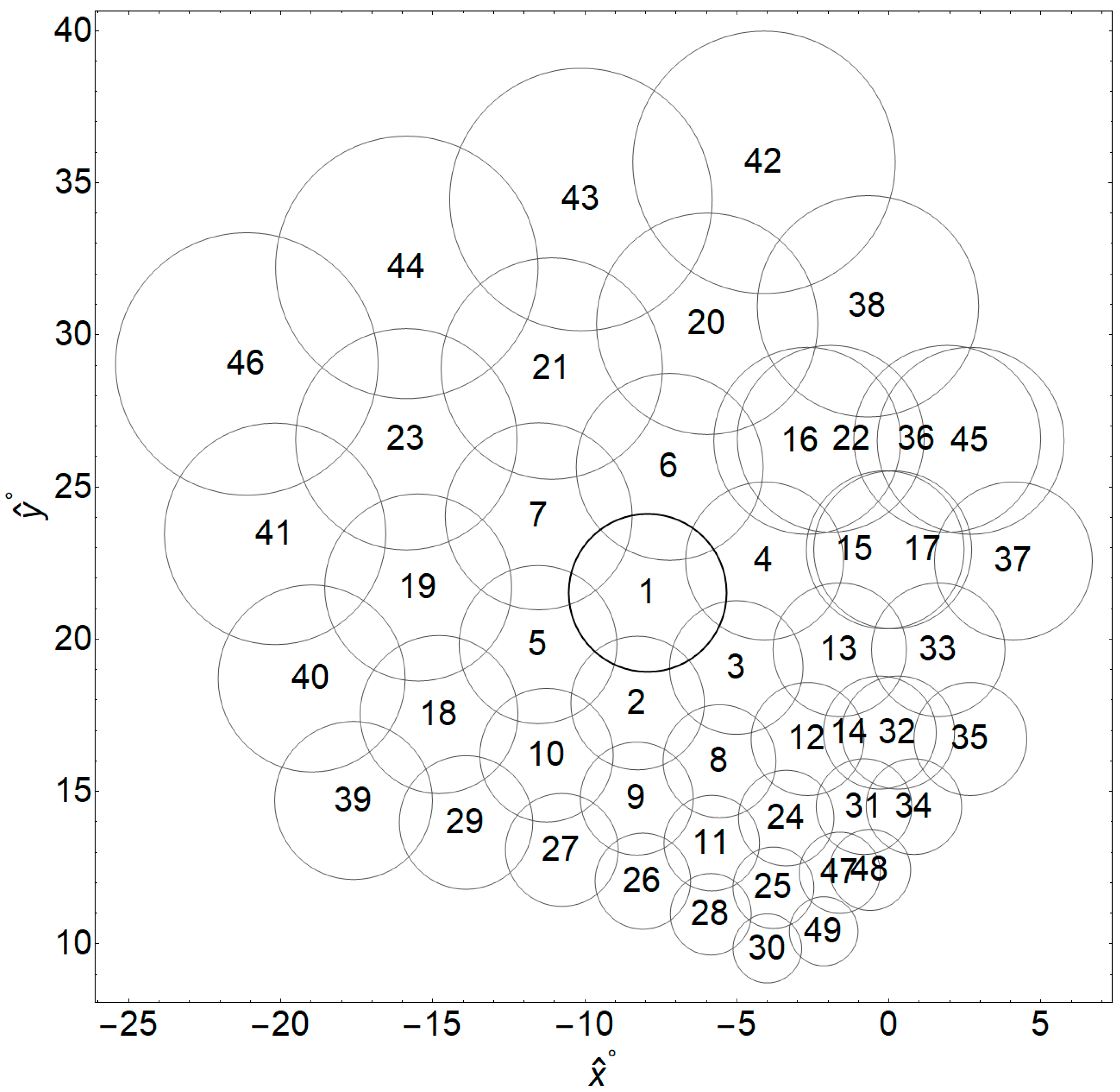
3.2. Simulations of a Neural Network Spanning 49 Cortical Columns Using NEST

Results found using $10 \mathrm{s}$ simulations of neurons in the 49 columns corresponding to the visual regions shown in Figure 2 are displayed in Figure 6 and Figure 7. Comparison of these results with Figure 4 and Figure 5 shows that nearly doubling the scale of the simulations produces qualitatively similar results. In particular, the percentage of time that neurons in all columns are active shows a great deal of variability prior to a large increase as the putative control parameter is increased, as it did for simulations of neurons in 25 columns. However, comparing Figure 6 with Figure 4 also shows that neurons in all columns become active for lower values of the putative control parameter as the number of columns simulated is increased.

Comparing Figure 7 with Figure 5 also demonstrates a difference in spike distributions. The overall number of spikes produced in all conditions is obviously higher when neurons in 49 columns are simulated. Overall mean numbers of spikes are consistent with this observation. The overall means for excitatory neurons are $132.26/\mathrm{s}$ in the absence of stimulation and $217.77/\mathrm{s}$ in the presence of stimulation, and for inhibitory neurons are $184.37/\mathrm{s}$ in the absence of stimulation and $329.46/\mathrm{s}$ in the presence of stimulation.

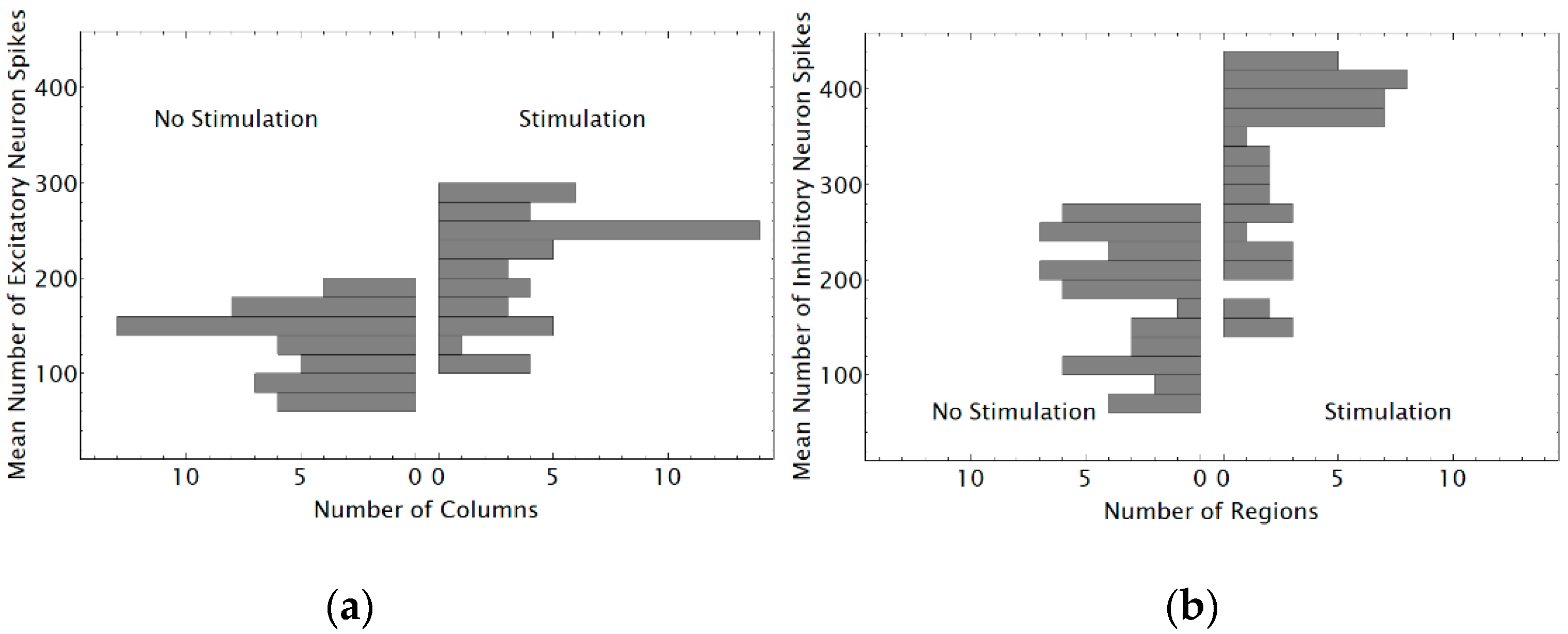
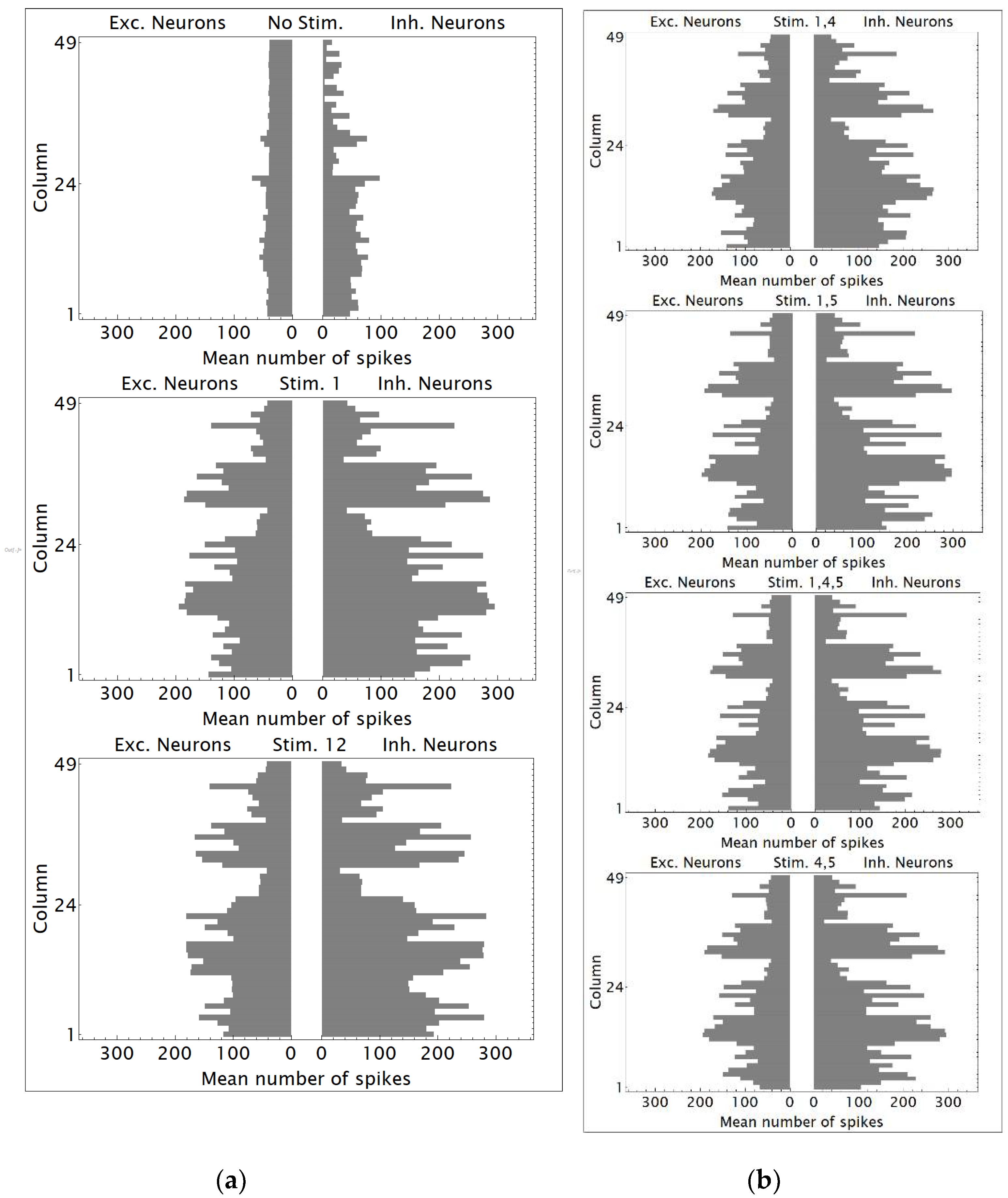
3.3. Using Distributions of Numbers of Spikes Produced by Neural Network Neurons to Detect the Number of Phosphenes

Multinomial logistic regression was used to determine if an accurate classification of the expected number of phosphenes could be produced using distributions of the numbers of spikes produced in 1$\mathrm{s}$ intervals of simulations of $10 \mathrm{s}$ duration by pairs of excitatory and inhibitory neurons in all 49 columns as predictor variables. The number of spikes produced by a specific excitatory neuron and the number of spikes produced by a specific inhibitory neuron in each column during a given simulation are combined to form a 98-element vector that is a “feature” employed for determining the number of phosphenes that are present during that second of the simulation. A single $1 \mathrm{s}$ simulation of neurons in 49 columns then produces 98 features that can be used for classification for each specific pair of an excitatory neuron and an inhibitory neuron, and there are 8 possible pairings of the 4 excitatory and 2 inhibitory neurons. As indicated in Section 2.3 and illustrated in Table 2, a total of 2080 examples consisting of vectors of numbers of spikes and a classification as “0”, “1”, “2”, or “3” phosphenes were used to develop a classification function for simulations in which the frequency of extrinsic, excitatory spikes was $40/\mathrm{s}$, $50/\mathrm{s}$, and $60/\mathrm{s}$. Half of the simulations employed G system synaptic strengths for the unaltered visual geometry shown in Figure 2 and half used G system synaptic strengths for an altered visual geometry in which regions 4 and 5 were each equal to the union of regions 1 and 4 and 5.

Examples of the mean number of spikes produced by the 4 excitatory neurons and 2 inhibitory neurons in each column during the first second of a $10 \mathrm{s}$ simulation for the unaltered visual geometry shown in Figure 2 during which 40 excitatory spikes/$\mathrm{s}$ were delivered to excitatory network neurons are shown in Figure 8. The cases depicted in Figure 8a were chosen because they illustrate dramatic differences in the spike distributions when no simulated stimulation is delivered (top panel) and when neurons in either column 1 (middle panel) or column 12 (bottom panel) are stimulated. The distributions shown in Figure 8b were chosen because they illustrate what appear to be cases for which correct classification of numbers of phosphenes may be much more challenging.

Visual regions 1 and 4 and regions 1 and 5 overlap, and therefore the cases in which columns that correspond to regions 1 and 4, 1 and 5, and 1, 4, and 5 are stimulated are all expected to give rise to a single phosphene. However, stimulation of the columns corresponding to visual regions 4 and 5, which do not overlap, is expected to give rise to two phosphenes.

Given the apparent difficulty of the classification task, it may be surprising that each of the 2080 classifications produced by the resulting classification function was correct for excitatory spike frequencies of $40/\mathrm{s}$, $50/\mathrm{s}$, and $60/\mathrm{s}$. Furthermore, the multinomial logistic regression model’s estimated conditional (posterior) probabilities of the correct number of phosphenes given each of the 2080 spike number examples are extremely high, as shown in Figure 9. The mean cross entropy values for simulations with excitatory spike frequencies of $40/\mathrm{s}$, $50/\mathrm{s}$, and $60/\mathrm{s}$ were $9.81\times {10}^{-5}$, $3.40\times {10}^{-6}$, and $6.81\times {10}^{-6}$, respectively. These data show that numbers of excitatory and inhibitory spikes can be used to classify the number of phosphenes with great accuracy even when the data arise from a mixture of visual geometries.

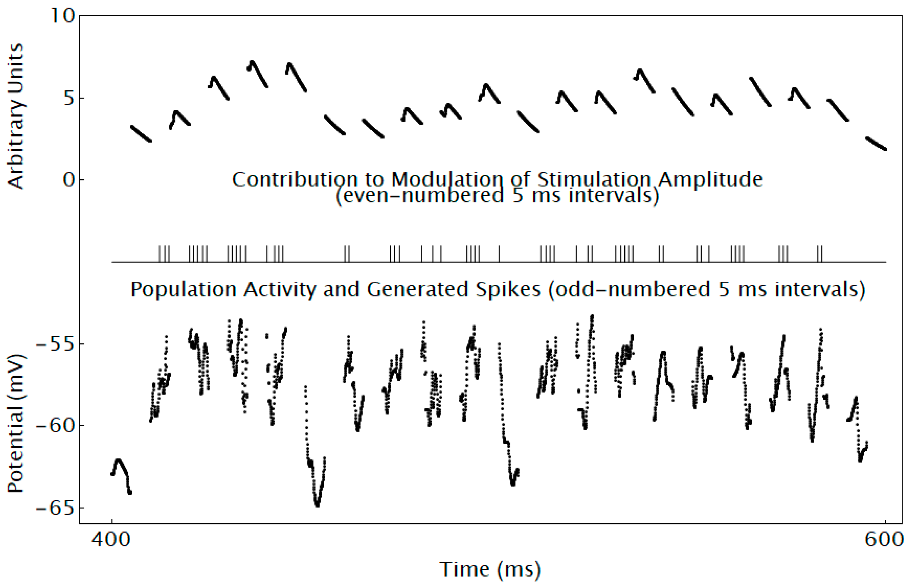
3.4. Simulating Essential Features of a Neuromorphic Device That Is Predicted to Engage Desired Visual Geometries

It was proposed in Section 1.4 that producing a second, desired visual geometry in order to alter phosphene shapes and sizes requires:

(1)

Intermittently recording activity from and stimulating each population for which an electrode is available;

(2)

Generating a neuromorphic spike if each recording of population activity is greater than a threshold;

(3)

Delivering neuromorphic spikes from all populations to a neuromorphic neuron that does not produce spikes for each population via neuromorphic G system conductance-based synapses; and

(4)

Using the membrane potential of each model neuron to determine the contribution of the recorded activity to modulation of stimulation amplitude for each population.

The essential functions of the proposed device were simulated using NEST and are illustrated in Figure 10 using data from a $1 \mathrm{s}$ simulation. In this simulation neurons in columns 1 and 12 received simulated stimulation, 40 extrinsic spikes/$\mathrm{s}$ were delivered to excitatory network neurons, G system synaptic strengths were based on the visual geometry that is illustrated in Figure 2, and the membrane potential of a single model neuron was recorded. Population activity of column 1 neurons was simulated by computing the average membrane potential of the 4 excitatory and 2 inhibitory neurons during odd-numbered $5 \mathrm{ms}$ intervals, thereby providing 100 samples for each such interval. A NEST spike generator produced a spike at time $t^{*}$ during an odd-numbered interval if simulated population activity was greater than a threshold of $-57 mV$ and at least $1 \mathrm{ms}$ had passed since the previous spike occurred. This threshold was found to yield a number of model spikes that is sufficient to provide a visualization of their impact on a model neuron’s membrane potential.

The spikes that were generated on odd-numbered $5 \mathrm{ms}$ intervals were delivered to an integrate and fire model neuron with 7 conductance-based synapses and excitatory G system strengths based on the visual geometry illustrated in Figure 2 on the subsequent even-numbered interval (i.e., at times $t^{*}+5 \mathrm{ms}$). The spike threshold for this neuron was set to $1000 \mathrm{mV}$ in order to ensure that no spikes were fired so that input merely modulated the neuron’s membrane potential. Inspection of Figure 10 shows that fluctuations in the simulated population activity produce corresponding changes in the population’s contribution to the modulation of stimulation amplitude.

4. Conclusions

NEST simulations of neurons in 25 columns run for $10 \mathrm{s}$ produce results that are qualitatively similar to $1 \mathrm{s}$ simulations that employ quantitatively different models of synapses and neurons. The most important result is that the effects of increasing the frequency of excitatory action potentials that are delivered to excitatory network neurons are consistent with the putative role of frequency as a control parameter for the engagement of the visual geometry and lightness interval distribution patterns. Differences between the initial, $1 \mathrm{s}$ simulations and the new, $10 \mathrm{s}$ NEST simulations are the onset of synaptic interactions among and between neurons in all 25 columns for lower values of this putative control parameter, higher frequencies of both excitatory and inhibitory network neuron action potentials, and overall higher spike frequencies for inhibitory rather than excitatory neurons. The higher spike frequencies suggest that it should be possible to employ fewer synapses and/or decreased synaptic strengths from the spike generators to excitatory network neurons in future simulations and neuromorphic emulations of the network.

Increasing the scale of simulations to 49 columns without adjusting any simulation parameters yielded qualitatively similar results to simulations of 25 columns. The frequency of extrinsic excitatory spikes again behaved in a manner that is consistent with the behavior of a control parameter, and the onset of interactions among and between neurons in all 49 columns occurred at still lower frequencies of this parameter. Frequencies of network neuron spikes were also higher than for the 25 column simulations. These results lead to an expectation that extrinsic excitatory spike frequency will continue to act as an order parameter as neurons in more columns are simulated. They also suggest that fewer synapses and/or lower synaptic strengths from spike generators to excitatory network neurons will very likely be necessary as the scale of simulations is further increased.

Multinomial logistic regression was applied to the problem of determining if distributions of numbers of spikes produced by the excitatory and inhibitory neurons that populate columns of the network can be used to determine the expected number of phosphenes produced by simulated stimulation of one or more columns. Results show that perfect classifications of phosphene numbers are found even though the data are derived from a mixture of visual geometries, and that the posterior probabilities of each number of phosphenes given an example of a spike number distribution are all close to 1. These results have important conceptual and practical implications. They are important conceptually because the contention that networks receiving spike trains from V1 produce patterns that include subjective awareness of the number of phosphenes and objective neural activity which is used to report that number behaviorally demands that such a classification is possible. They are important in a practical sense because they suggest that classifications produced using multinomial logistic regression can provide useful information regarding the performance of simulations of the sought-after neuromorphic device. For example, we should expect simulations that include this device together with the neural network to yield distributions of numbers of spikes for which highly accurate classifications of expected phosphene numbers are found. In particular, accurate classifications should result when the network G system synaptic strengths are based on the visual geometry illustrated in Figure 2 and when neuromorphic device G system synaptic strengths are based on both the same and on different visual geometries as the network. If classifications are initially inaccurate, it may be possible to improve them by altering parameters (other than G system synaptic strengths) of the neuromorphic device part of the simulation.

The basic and essential functions of the neuromorphic device as described in Section 1.4 and illustrated by Figure 3 were also simulated using NEST. It was shown that intermittent simulated stimulation of a population of neurons in each column for which an electrode is available can be modulated by the intermittently recorded electrical activity of each population in a way that is consistent with the stated requirements of the device.

5. Future Work

There are several reasons for following up the work reported here with additional simulations that include essential features of the neuromorphic device before increasing the scale of simulations. The first reason has to do with performance of the multinomial logistic regression classification. As noted in Section 2.2, 95 additional spikes were always added to spike numbers for neurons in columns receiving simulated electrical stimulation, and it is hardly likely that such a noise-free situation is the case in a biological neural network. Furthermore, simulating the neuromorphic device requires simulating the delivery of current that is above the threshold for producing a phosphene in a small number of columns and simulating current that is below this threshold in all remaining columns with an electrode as described in Section 1.4. It is important to determine how a multinomial logistic regression classification performs if additional, randomly varying numbers of spikes are produced in all columns having electrodes, with the mean number being larger for columns receiving stimulation above the threshold for producing phosphenes.

Second, although few surprises are expected as the scale of the neural network simulations is increased, virtually nothing is known regarding overall performance of a simulation that includes code for the neuromorphic device. In order to make performance of these simulations as easy to understand as possible, it is wise to break up each simulation into $5 \mathrm{ms}$ intervals. During odd-numbered intervals population recordings from columns, generation of neuromorphic spikes, delivery of spikes to G system synapses, and computation of membrane potential for each neuromorphic neuron can be simulated. During even-numbered intervals, the membrane potential values can be applied to modulation of stimulation of each column. These additional steps will add to the computational load and duration of each simulation, and will have increasingly significant effects as the number of stimulated columns being simulated is increased.

The potential utility of understanding how distributions of numbers of spikes produced by network neurons can be used to classify the number of phosphenes provides a third reason. In order for an emulation of the neuromorphic device to perform as desired, producing visual geometries that have the objective of improving object recognition must alter spike number distributions that can be used to accurately classify the intended resulting number of phosphenes. Although classifications that are made using multinomial logistic regression provide information on accuracy, accuracy alone is of limited utility with regard to deciding how to change simulation parameters in order to improve accuracy. Understanding the information that is provided by features of spike number distributions would be more informative. For example, it may be the case that phosphene classification depends on information regarding the visual geometry and on information regarding the lightness interval distribution, and that different features of the spike number distributions yield these two types of information. In this case, it would be possible to examine spike number distributions in order to determine whether poor classification using the neuromorphic device results from one of the two features, or from both features of the distributions. Having knowledge of required changes in spike number distributions would be very helpful in deciding which parameters of simulations to change.

Increasing the scale of simulations that include simulations of the sought-after neuromorphic device should be fairly straightforward if the desired visual geometries yield accurate classifications of the expected numbers of phosphenes. These simulations can then be followed by emulation of neurons in all columns of the network together with emulation of the device using neuromorphic hardware. The increase in speed provided by neuromorphic hardware [39] should make it possible to gather data that are expected to be particularly helpful in designing human research that employs a neuromorphic device. For example, the emulated cortical columns that receive stimulation current can be chosen so that the expected positions of phosphenes fall close to edges of an object as defined by output of an event-based sensor [28]. Comparisons of the expected visual experiences that result from emulations which do and do not include the neuromorphic device could then be made.

6. Patents

A provisional patent application for the sense element engagement process has been submitted [35]. A second provisional patent application for the material provided in this paper has been submitted [44].

References

1. Button, J.C. Electronics brings light to the blind. Radio Electron. 1958, 29, 53–55. [Google Scholar]
2. Bourne, R.R.A.; Flaxman, S.R.; Braithwaite, T.; Cicinelli, M.V.; Das, A.; Jonas, J.B.; Keeffe, J.; Kempen, J.H.; Leasher, J.; Limburg, H.; et al. Magnitude, temporal trends, and projections of the global prevalence of blindness and distance and near vision impairment: A systematic review and meta-analysis. Lancet Glob. Health 2017, 5, e888–e897. [Google Scholar] [CrossRef]
3. Varma, R.; Vajaranant, T.S.; Burkemper, B.; Wu, S.; Torres, M.; Hsu, C.; Choudhury, F.; McKean-Cowdin, R. Visual impair-ment and blindness in adults in the United States: Demographic and geographic variations from 2015–2050. JAMA Ophthal-Mol. 2016, 134, 802–809. [Google Scholar] [CrossRef]
4. Lewis, P.M.; Rosenfeld, J.V. Electrical stimulation of the brain and the development of cortical visual prostheses: An historical perspective. Brain Res. 2016, 1630, 208–224. [Google Scholar] [CrossRef] [PubMed]
5. Niketeghad, S.; Pouratian, N. Brain Machine Interfaces for Vision Restoration: The Current State of Cortical Visual Prosthetics. Neurotherapeutics 2018, 16, 134–143. [Google Scholar] [CrossRef]
6. Roe, A.W.; Chen, G.; Xu, A.G.; Hu, J. A roadmap to a columnar visual cortical prosthetic. Curr. Opin. Physiol. 2020, 16, 68–78. [Google Scholar] [CrossRef]
7. de Vries, S.E.J.; Lecoq, J.A.; Buice, M.A.; Groblewski, P.A.; Ocker, G.K.; Oliver, M.; Feng, D.; Cain, N.; Ledochowitsch, P.; Millman, D.; et al. A large-scale standardized physiological survey reveals functional organization of the mouse visual cortex. Nat. Neurosci. 2019, 23, 138–151. [Google Scholar] [CrossRef] [PubMed]
8. Olshausen, B.A.; Field, D.G. How close are we to understanding V1? Neural Comput. 2005, 17, 1665–1699. [Google Scholar] [CrossRef]
9. Chalmers, D.J. Facing up to the problem of consciousness. J. Conscious. Stud. 1995, 2, 200–219. [Google Scholar]
10. Chalmers, D.J. The Conscious Mind: In Search of a Fundamental Theory; Oxford University Press: New York, NY, USA, 1996. [Google Scholar]
11. Seth, A.K.; Bayne, T. Theories of consciousness. Nat. Rev. Neurosci. 2022, 23, 439–452. [Google Scholar] [CrossRef]
12. Gutierrez, G. Orion Shines a Light in the Dark for the Blind, Baylor College of Medicine Blog. July 2019. Available online: https://blogs.bcm.edu/2019/07/11/from-the-labs-orion-turns-on-a-light-in-the-dark-for-the-blind/ (accessed on 30 September 2022).
13. Fernández, E.; Normann, R.A. Cortivis approach for an intracortical visual prosthesis. In Artificial Vision: A Clinical Guide; Gabel, V.P., Ed.; Springer: Munich, Germany, 2017; pp. 191–201. [Google Scholar]
14. Lowery, A.J.; Rosenfeld, J.V.; Rosa, M.G.P.; Brunton, E.; Rajan, R.; Mann, C.; Armstrong, M.; Mohan, A.; Josh, H.; Kleeman, L.; et al. Monash Vision Group’s Gennaris Cortical Implant for Vision Restoration. In Artificial Vision: A Clinical Guide; Gabel, V.P., Ed.; Springer: Munich, Germany, 2017; pp. 215–225. [Google Scholar]
15. Troyk, P.R. The intracortical visual prosthesis project. In Artificial Vision: A Clinical Guide; Gabel, V.P., Ed.; Springer: Munich, Germany, 2017; pp. 203–214. [Google Scholar]
16. Schiller, P.H.; Tehovnik, E.J. Visual Prosthesis. Perception 2008, 37, 1529–1559. [Google Scholar] [CrossRef] [PubMed]
17. Komarov, M.; Malerba, P.; Golden, R.; Nunez, P.; Halgren, E.; Bazhenov, M. Selective recruitment of cortical neurons by electrical stimulation. PLoS Comput. Biol. 2019, 15, e1007277. [Google Scholar] [CrossRef] [PubMed]
18. Rattay, F. The basic mechanism for the electrical stimulation of the nervous system. Neuroscience 1999, 89, 335–346. [Google Scholar] [CrossRef]
19. Tootell, R.B.H.; Silverman, M.S.; Switkes, E.; De Valois, R.L. Deoxyglucose Analysis of Retinotopic Organization in Primate Striate Cortex. Science 1982, 218, 902–904. [Google Scholar] [CrossRef] [PubMed]
20. Bosking, W.H.; Beauchamp, M.S.; Yoshor, D. Electrical Stimulation of Visual Cortex: Relevance for the Development of Visual Cortical Prosthetics. Annu. Rev. Vis. Sci. 2017, 3, 141–166. [Google Scholar] [CrossRef] [PubMed]
21. Bak, M.; Girvin, J.P.; Hambrecht, F.T.; Kufta, C.V.; Loeb, G.E.; Schmidt, E.M. Visual sensations produced by intracortical microstimulation of the human occipital cortex. Med. Biol. Eng. Comput. 1990, 28, 257–259. [Google Scholar] [CrossRef]
22. Beauchamp, M.S.; Oswalt, D.; Sun, P.; Foster, B.L.; Magnotti, J.F.; Niketeghad, S.; Pouratian, N.; Bosking, W.H.; Yoshor, D. Dynamic Stimulation of Visual Cortex Produces Form Vision in Sighted and Blind Humans. Cell 2020, 181, 774–783.e5. [Google Scholar] [CrossRef]
23. Brindley, G.S.; Lewin, W.S. The sensations produced by electrical stimulation of the visual cortex. J. Physiol. 1968, 196, 479–493. [Google Scholar] [CrossRef]
24. Doebelle, W.H. Artificial vision for the blind by connecting a television camera to the visual cortex. Am. Soc. Artif. Intern. Organs J. 2000, 46, 3–9. [Google Scholar] [CrossRef]
25. Dobelle, W.H.; Quest, D.O.; Antunes, J.L.; Roberts, T.S.; Girvin, J.P. Artificial Vision for the Blind by Electrical Stimulation of the Visual Cortex. Neurosurgery 1979, 5, 521–527. [Google Scholar] [CrossRef]
26. Schmidt, E.M.; Bak, M.J.; Hambrecht, F.T.; Kufta, C.V.; O’Rourke, D.K.; Vallabhanath, P. Feasibility of a visual prosthesis for the blind based on intracortical micro stimulation of the visual cortex. Brain 1996, 119, 507–522. [Google Scholar] [CrossRef] [PubMed]
27. Rushton, D.N.; Brindley, G.S. Short- and long-term stability of cortical electrical phosphenes. In Physiological Aspects of Clinical Neurology; Rose, R.C., Ed.; Blackwell Scientific Publishing: London, UK, 1997; pp. 123–153. [Google Scholar]
28. Sahel, J.-A.; Boulanger-Scemama, E.; Pagot, C.; Arleo, A.; Galluppi, F.; Martel, J.N.; Degli Esposti, S.; Delaux, A.; de Saint Aubert, J.-B.; de Montleau, C.; et al. Partial recovery of visual function in a blind patient after optogenetic therapy. Nat. Med. 2021, 27, 1223–1229. [Google Scholar] [CrossRef] [PubMed]
29. Dobelle, W.H.; Mladejovsky, M.G. Phosphenes produced by electrical stimulation of human occipital cortex, and their application to the development of a prosthesis for the blind. J. Physiol. 1974, 243, 553–576. [Google Scholar] [CrossRef]
30. Caspi, A.; Barry, M.P.; Patel, U.K.; Salas, M.A.; Dorn, J.D.; Roy, A.; Niketeghad, S.; Greenberg, R.J.; Pouratian, N. Eye movements and the perceived location of phosphenes generated by intracranial primary visual cortex stimulation in the blind. Brain Stimul. 2021, 14, 851–860. [Google Scholar] [CrossRef] [PubMed]
31. Caspi, A.; Roy, A.; Wuyyuru, V.; Rosendall, P.E.; Harper, J.W.; Katyal, K.D.; Barry, M.P.; Dagnelie, G.; Greenberg, R.J. Eye Movement Control in the Argus II Retinal-Prosthesis Enables Reduced Head Movement and Better Localization Precision. Investig. Ophthalmol. Vis. Sci. 2018, 59, 792–802. [Google Scholar] [CrossRef]
32. Bosking, W.H.; Sun, P.; Ozker, M.; Pei, X.; Foster, B.L.; Beauchamp, M.S.; Yoshor, D. Saturation in Phosphene Size with Increasing Current Levels Delivered to Human Visual Cortex. J. Neurosci. 2017, 37, 7188–7197. [Google Scholar] [CrossRef] [PubMed]
33. Tehovnik, E.J.; Slocum, W.M. Phosphene induction by microstimulation of macaque V1. Brain Res. Rev. 2007, 53, 337–343. [Google Scholar] [CrossRef]
34. Dayan, P.; Abbott, L.F. Theoretical Neuroscience: Computational and Mathematical Modeling of Neural Systems; The MIT Press: Cambridge, MA, USA, 2001. [Google Scholar]
35. Pavloski, R. Sense Element Engagement Theory Explains How Neural Networks Produce Cortical Prosthetic Vision. U.S. Provisional Patent Application No. 63/287,286, 8 December 2021. [Google Scholar]
36. Pavloski, R. Sense Element Engagement Theory Explains How Neural Networks Produce Cortical Prosthetic Vision. IEEE Trans. Neural Netw. Learn. Syst. 2021; Submitted. Available online: https://www.techrxiv.org/articles/preprint/Sense_Element_Engagement_Theory_Explains_How_Neural_Networks_Produce_Cortical_Prosthetic_Vision/17161187/1(accessed on 30 September 2022).
37. Schöner, G.; Kelso, J.A.S. Dynamic Pattern Generation in Behavioral and Neural Systems. Science 1988, 239, 1513–1520. [Google Scholar] [CrossRef]
38. Kelso, J.A.S. Dynamic Patterns: The Self-Organization of Brain and Behavior; The MIT Press: Cambridge, MA, USA, 1995. [Google Scholar]
39. Pehle, C.; Billaudelle, S.; Cramer, B.; Kaiser, J.; Schreiber, K.; Stradmann, Y.; Weis, J.; Leibfried, A.; Müller, E.; Schemmel, J. The BrainScaleS-2 Accelerated Neuromorphic System With Hybrid Plasticity. Front. Neurosci. 2022, 16, 795876. [Google Scholar] [CrossRef]
40. Eppler, J.M.; Helias, M.; Muller, E.; Diesmann, M.; Gewaltig, M.-O. PyNEST: A convenient interface to the NEST simulator. Front. Neuroinf. 2008, 2, 12. [Google Scholar] [CrossRef] [PubMed]
41. Fardet, T.; Vennemo, S.B.; Mitchell, J.; Mørk, H.; Graber, S.; Hahne, J.; Spreizer, S.; Deepu, R.; Trensch, G.; Weidel, P.; et al. NEST 2.20.0 (2.20.0). Zenodo. Available online: https://doi.org/10.5281/zenodo.3605514 (accessed on 30 September 2022).
42. Xu, Z.; Tao, D.; Zhang, Y.; Wu, J.; Tsoi, A.C. Architectural Style Classification Using Multinomial Latent Logistic Regression. In LNCS 8689—Architectural Style Classification Using Multinomial Latent Logistic Regression; Fleet, D., Ed.; ECCV: 2014; Springer International Publishing: Cham, Switzerland, 2014; Available online: https://springer.com (accessed on 30 September 2022).
43. Saputro, D.R.S.; Widyaningsih, P. Limited memory Broyden-Fletcher-Goldfarb-Shanno (L-BFGS) method for the parameter estimation on geographically weighted ordinal logistic regression model (GWOLR). In AIP Conference Proceedings; AIP Publishing LLC: Melville, NY, USA, 2017; Volume 1868, p. 040009. [Google Scholar] [CrossRef]
44. Pavloski, R. Progress in Developing a Neuromorphic Device That Is Predicted to Enhance Cortical Prosthetic Vision by Enabling the Formation of Multiple Visual Geometries. U.S. Provisional Patent Application No. 63/354,959, 23 June 2022. [Google Scholar]
Figure 1. An idealized V1 geometry consisting of 939 columns in which negative values of x are used for the left hemisphere is shown in panel (a) and a corresponding idealized visual geometry consisting of 939 visual regions in which negative values of x ^ ° denote the left visual field is shown in (b). The darker columns and corresponding regions are employed in computer simulations. This figure was constructed in the same fashion as Figure 2 in [35,36] but identifies 49 rather than 25 columns and corresponding visual regions that are included in simulations.
Prosthesis 04 00049 g001
Figure 2. Visual regions corresponding to columns containing neurons that are used in computer simulations are shown using a numbering convention that is described in Section 2.2. Small-scale simulations of a network consisting of neurons in columns corresponding to regions 1–25 are reported in [35,36] and are replicated here. Additional research reported in the present paper is based on simulations of neurons in columns corresponding to all 49 regions that are depicted here.
Prosthesis 04 00049 g002
Figure 3. A simple block diagram illustrates essential features of how a neuromorphic device is proposed to complement a currently available CPV system. Each of the stimulation units receives input from the CPV system’s microprocessor which in turn receives video input and produces a mean stimulation amplitude that is either below or above the threshold for producing a phosphene. Neuromorphic G system synapses receive input from all neuromorphic spike generators but only connections to synapses for column 1 are shown.
Prosthesis 04 00049 g003
Figure 4. The percentage of the final 900 ms of each of 10, 1 s segments of 10 s simulations during which excitatory (closed disks) and inhibitory (open squares) neurons in all 25 columns are producing non-zero values in synaptic conductance in target neurons. Lines join values averaged over the 10, 1 s intervals. Panel (a) depicts data in the absence of simulated stimulation and panel (b) shows data in the presence of simulated stimulation of column 1 neurons.
Prosthesis 04 00049 g004
Figure 5. The distributions of numbers of spikes for network excitatory (a) and inhibitory (b) neurons in columns 1–25 averaged over 10 s simulations are shown for both no stimulation and stimulation conditions. The frequency of extrinsic excitatory action potentials was set to 70 / s .
Prosthesis 04 00049 g005
Figure 6. The results reported in Figure 4 for simulations of neurons in 25 columns are shown here for simulations of neurons in 49 columns. Although the general shapes of the average values joined by lines are similar to those found for 25 columns, the onset of continuously active neurons in all columns occurs for lower values of the control parameter. Panel (a) depicts data in the absence of simulated stimulation and panel (b) shows data in the presence of simulated stimulation of column 1 neurons.
Prosthesis 04 00049 g006
Figure 7. The distributions of numbers of spikes for network excitatory (a) and inhibitory (b) neurons in columns 1–49 averaged over 10 s simulations are shown for both no stimulation and stimulation conditions. The frequency of extrinsic excitatory action potentials was set to 70 / s .
Prosthesis 04 00049 g007
Figure 8. Examples of distributions of mean numbers of spikes produced by the neurons in each column during the first second of a 10 s simulation in which 40 excitatory spikes/s were delivered to excitatory network neurons. (a) There are clear differences between the distributions in (a) but those in (b) appear to be more similar and suggest that correct classification of the expected number of phosphenes would be difficult.
Prosthesis 04 00049 g008
Figure 9. The frequency of occurrence of all posterior probability estimates for correct choices given each of the 2080 examples are shown for simulations in which the control parameter has values of 40/ s , 50/s, and 60/s. Bin widths are 5.7777 × 10⁻⁴, 5.7943 × 10⁻⁵, and 1.2255 × 10⁻⁴ from top to bottom.
Prosthesis 04 00049 g009
Figure 10. Simulated activity of column 1 neurons and simulated spikes resulting from values greater than 57   mV are shown during odd-numbered 5 ms intervals, and the membrane potential of a model neuron that is influenced by these spikes via G system synapses is shown during even-numbered 5 ms intervals. Data are displayed for 200 ms in order to provide a clear visualization of the data for each interval and the impact of spikes on the contribution of column 1 activity to modulation of intermittent stimulation of column 1 neurons.
Prosthesis 04 00049 g010