
Model-Free Deep Recurrent Q-Network Reinforcement Learning for Quantum Circuit Architectures Design
 ,
,
Abstract
:1. Introduction
2. Methods
2.1. MDP, POMDP, and QOMDP
2.2. LSTM-Based Deep Recurrent Q-Network
2.3. RL Method
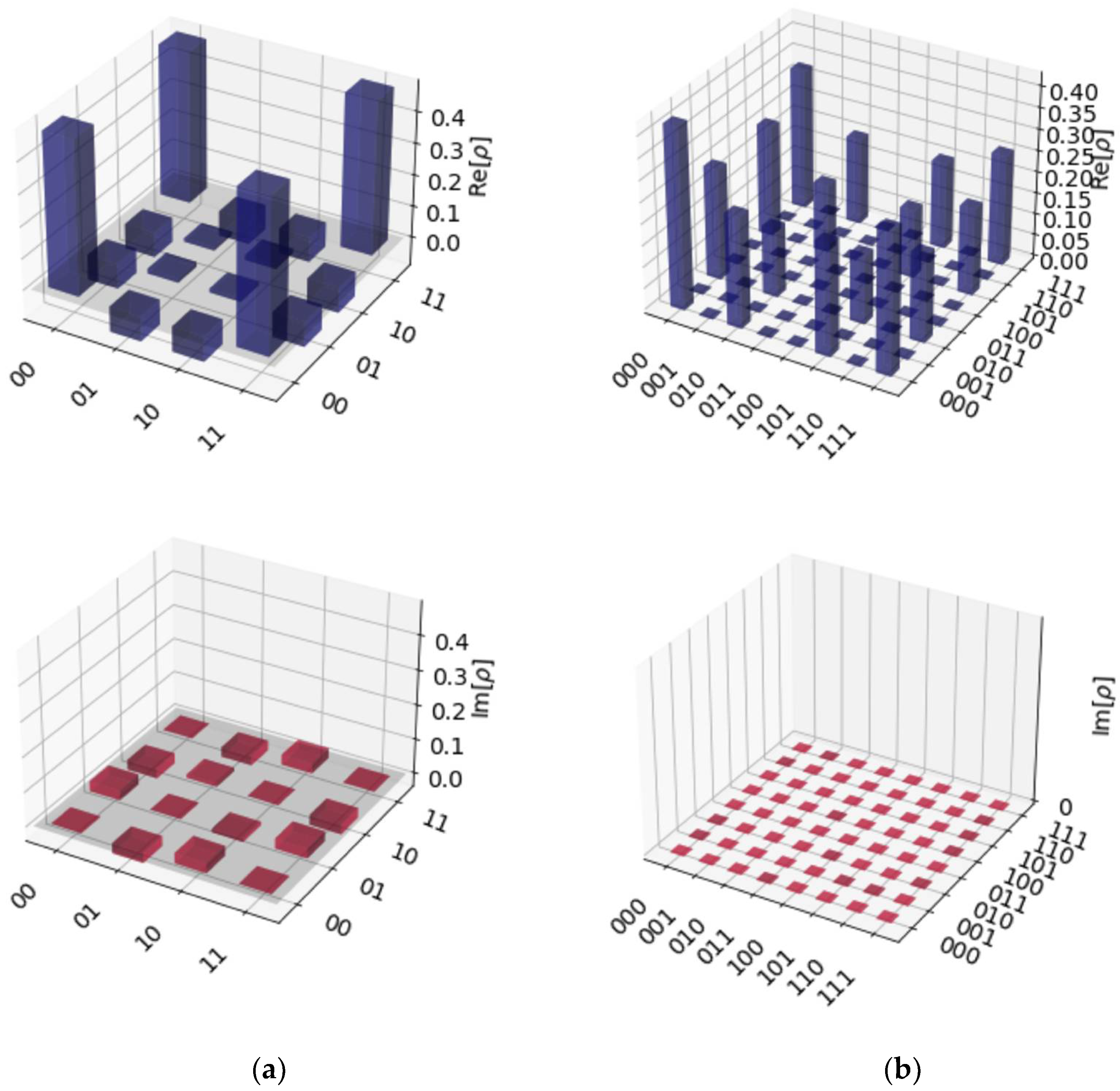
3. Results
4. Discussion
5. Conclusions
Author Contributions
Funding
Institutional Review Board Statement
Informed Consent Statement
Data Availability Statement
Acknowledgments
Conflicts of Interest
References
- Dunjko, V.; Briegel, H.J. Machine learning & artificial intelligence in the quantum domain: A review of recent progress. Rep. Prog. Phys. 2018, 81, 074001. [Google Scholar] [CrossRef] [PubMed]
- Preskill, J. Quantum Computing in the NISQ era and beyond. Quantum 2018, 2, 79. [Google Scholar] [CrossRef]
- Wiseman, H.M.; Milburn, G.J. Quantum Measurement and Control; Cambridge University Press: Cambridge, UK, 2009; ISBN 978-0-521-80442-4. [Google Scholar]
- Nurdin, H.I.; Yamamoto, N. Linear Dynamical Quantum Systems: Analysis, Synthesis, and Control, 1st ed; Springer: New York, NY, USA, 2017; ISBN 978-3-319-55199-9. [Google Scholar]
- Johansson, J.R.; Nation, P.D.; Nori, F. QuTiP 2: A Python framework for the dynamics of open quantum systems. Comput. Phys. Commun. 2013, 184, 1234–1240. [Google Scholar] [CrossRef]
- Sutton, R.S.; Barto, A.G. Reinforcement Learning: An Introduction, 2nd ed.; Adaptive Computation and Machine Learning Series; Bradford Books: Cambridge, MA, USA, 2018; ISBN 978-0-262-03924-6. [Google Scholar]
- Russell, S.; Norvig, P. Artificial Intelligence: A Modern Approach, 4th ed.Pearson Education Limited: London, UK, 2021; ISBN 978-1-292-40113-3. [Google Scholar]
- Szepesvari, C. Algorithms for Reinforcement Learning, 1st ed.Morgan and Claypool Publishers: San Rafael, CA, USA, 2010; ISBN 978-1-60845-492-1. [Google Scholar]
- Kaelbling, L.P.; Littman, M.L.; Moore, A.W. Reinforcement Learning: A Survey. J. Artif. Intell. Res. 1996, 4, 237–285. [Google Scholar] [CrossRef]
- Geramifard, A.; Walsh, T.J.; Tellex, S.; Chowdhary, G.; Roy, N.; How, J.P. A Tutorial on Linear Function Approximators for Dynamic Programming and Reinforcement Learning. Found. Trends® Mach. Learn. 2013, 6, 375–451. [Google Scholar] [CrossRef]
- Mnih, V.; Kavukcuoglu, K.; Silver, D.; Rusu, A.A.; Veness, J.; Bellemare, M.G.; Graves, A.; Riedmiller, M.; Fidjeland, A.K.; Ostrovski, G.; et al. Human-level control through deep reinforcement learning. Nature 2015, 518, 529–533. [Google Scholar] [CrossRef]
- Watkins, C.J.C.H.; Dayan, P. Q-learning. Mach. Learn. 1992, 8, 279–292. [Google Scholar] [CrossRef]
- Silver, D.; Schrittwieser, J.; Simonyan, K.; Antonoglou, I.; Huang, A.; Guez, A.; Hubert, T.; Baker, L.; Lai, M.; Bolton, A.; et al. Mastering the game of Go without human knowledge. Nature 2017, 550, 354–359. [Google Scholar] [CrossRef]
- Bellman, R. Dynamic Programming; Reprint Edition; Dover Publications: Mineola, NY, USA, 2003; ISBN 978-0-486-42809-3. [Google Scholar]
- Aoki, M. Optimal control of partially observable Markovian systems. J. Frankl. Inst. 1965, 280, 367–386. [Google Scholar] [CrossRef]
- Åström, K.J. Optimal control of Markov processes with incomplete state information. J. Math. Anal. Appl. 1965, 10, 174–205. [Google Scholar] [CrossRef] [Green Version]
- Papadimitriou, C.H.; Tsitsiklis, J.N. The Complexity of Markov Decision Processes. Math. Oper. Res. 1987, 12, 441–450. [Google Scholar] [CrossRef]
- Xiang, X.; Foo, S. Recent Advances in Deep Reinforcement Learning Applications for Solving Partially Observable Markov Decision Processes (POMDP) Problems: Part 1—Fundamentals and Applications in Games, Robotics and Natural Language Processing. Mach. Learn. Knowl. Extr. 2021, 3, 554–581. [Google Scholar] [CrossRef]
- Kimura, T.; Shiba, K.; Chen, C.-C.; Sogabe, M.; Sakamoto, K.; Sogabe, T. Variational Quantum Circuit-Based Reinforcement Learning for POMDP and Experimental Implementation. Math. Probl. Eng. 2021, 2021, 3511029. [Google Scholar] [CrossRef]
- Kaelbling, L.P.; Littman, M.L.; Cassandra, A.R. Planning and acting in partially observable stochastic domains. Artif. Intell. 1998, 101, 99–134. [Google Scholar] [CrossRef]
- Singh, S.P.; Jaakkola, T.; Jordan, M.I. Learning without State-Estimation in Partially Observable Markovian Decision Processes. In Machine Learning Proceedings 1994; Cohen, W.W., Hirsh, H., Eds.; Morgan Kaufmann: San Francisco, CA, USA, 1994; pp. 284–292. ISBN 978-1-55860-335-6. [Google Scholar]
- Barry, J.; Barry, D.T.; Aaronson, S. Quantum partially observable Markov decision processes. Phys. Rev. A 2014, 90, 032311. [Google Scholar] [CrossRef]
- Ying, S.; Ying, M. Reachability analysis of quantum Markov decision processes. Inf. Comput. 2018, 263, 31–51. [Google Scholar] [CrossRef]
- Ying, M.-S.; Feng, Y.; Ying, S.-G. Optimal Policies for Quantum Markov Decision Processes. Int. J. Autom. Comput. 2021, 18, 410–421. [Google Scholar] [CrossRef]
- Abhijith, J.; Adedoyin, A.; Ambrosiano, J.; Anisimov, P.; Casper, W.; Chennupati, G.; Coffrin, C.; Djidjev, H.; Gunter, D.; Karra, S.; et al. Quantum Algorithm Implementations for Beginners. ACM Trans. Quantum Comput. 2022, 3, 18:1–18:92. [Google Scholar] [CrossRef]
- Cerezo, M.; Arrasmith, A.; Babbush, R.; Benjamin, S.C.; Endo, S.; Fujii, K.; McClean, J.R.; Mitarai, K.; Yuan, X.; Cincio, L.; et al. Variational quantum algorithms. Nat. Rev. Phys. 2021, 3, 625–644. [Google Scholar] [CrossRef]
- Nielsen, M.A.; Chuang, I.L. Quantum Computation and Quantum Information: 10th Anniversary Edition. Available online: https://www.cambridge.org/highereducation/books/quantum-computation-and-quantum-information/01E10196D0A682A6AEFFEA52D53BE9AE (accessed on 22 August 2022).
- Barenco, A.; Bennett, C.H.; Cleve, R.; DiVincenzo, D.P.; Margolus, N.; Shor, P.; Sleator, T.; Smolin, J.A.; Weinfurter, H. Elementary gates for quantum computation. Phys. Rev. A 1995, 52, 3457–3467. [Google Scholar] [CrossRef] [Green Version]
- Deutsch, D. Quantum theory, the Church–Turing principle and the universal quantum computer. Proc. R. Soc. Lond. Math. Phys. Sci. 1985, 400, 97–117. [Google Scholar] [CrossRef]
- Feynman, R.P. Simulating physics with computers. Int. J. Theor. Phys. 1982, 21, 467–488. [Google Scholar] [CrossRef]
- Mermin, N.D. Quantum Computer Science: An Introduction; Cambridge University Press: Cambridge, UK, 2007; ISBN 978-0-521-87658-2. [Google Scholar]
- Arute, F.; Arya, K.; Babbush, R.; Bacon, D.; Bardin, J.C.; Barends, R.; Biswas, R.; Boixo, S.; Brandao, F.G.S.L.; Buell, D.A.; et al. Quantum supremacy using a programmable superconducting processor. Nature 2019, 574, 505–510. [Google Scholar] [CrossRef] [PubMed]
- Chen, C.-C.; Shiau, S.-Y.; Wu, M.-F.; Wu, Y.-R. Hybrid classical-quantum linear solver using Noisy Intermediate-Scale Quantum machines. Sci. Rep. 2019, 9, 16251. [Google Scholar] [CrossRef] [PubMed]
- Kimura, T.; Shiba, K.; Chen, C.-C.; Sogabe, M.; Sakamoto, K.; Sogabe, T. Quantum circuit architectures via quantum observable Markov decision process planning. J. Phys. Commun. 2022, 6, 075006. [Google Scholar] [CrossRef]
- Borah, S.; Sarma, B.; Kewming, M.; Milburn, G.J.; Twamley, J. Measurement-Based Feedback Quantum Control with Deep Reinforcement Learning for a Double-Well Nonlinear Potential. Phys. Rev. Lett. 2021, 127, 190403. [Google Scholar] [CrossRef]
- Sivak, V.V.; Eickbusch, A.; Liu, H.; Royer, B.; Tsioutsios, I.; Devoret, M.H. Model-Free Quantum Control with Reinforcement Learning. Phys. Rev. X 2022, 12, 011059. [Google Scholar] [CrossRef]
- Niu, M.Y.; Boixo, S.; Smelyanskiy, V.N.; Neven, H. Universal quantum control through deep reinforcement learning. NPJ Quantum Inf. 2019, 5, 33. [Google Scholar] [CrossRef]
- He, R.-H.; Wang, R.; Nie, S.-S.; Wu, J.; Zhang, J.-H.; Wang, Z.-M. Deep reinforcement learning for universal quantum state preparation via dynamic pulse control. EPJ Quantum Technol. 2021, 8, 29. [Google Scholar] [CrossRef]
- Bukov, M.; Day, A.G.R.; Sels, D.; Weinberg, P.; Polkovnikov, A.; Mehta, P. Reinforcement Learning in Different Phases of Quantum Control. Phys. Rev. X 2018, 8, 031086. [Google Scholar] [CrossRef] [Green Version]
- Mackeprang, J.; Dasari, D.B.R.; Wrachtrup, J. A reinforcement learning approach for quantum state engineering. Quantum Mach. Intell. 2020, 2, 5. [Google Scholar] [CrossRef]
- Zhang, X.-M.; Wei, Z.; Asad, R.; Yang, X.-C.; Wang, X. When does reinforcement learning stand out in quantum control? A comparative study on state preparation. NPJ Quantum Inf. 2019, 5, 1–7. [Google Scholar] [CrossRef]
- Baum, Y.; Amico, M.; Howell, S.; Hush, M.; Liuzzi, M.; Mundada, P.; Merkh, T.; Carvalho, A.R.R.; Biercuk, M.J. Experimental Deep Reinforcement Learning for Error-Robust Gate-Set Design on a Superconducting Quantum Computer. PRX Quantum 2021, 2, 040324. [Google Scholar] [CrossRef]
- Kuo, E.-J.; Fang, Y.-L.L.; Chen, S.Y.-C. Quantum Architecture Search via Deep Reinforcement Learning. arXiv 2021, arXiv:2104.07715. [Google Scholar]
- Pirhooshyaran, M.; Terlaky, T. Quantum circuit design search. Quantum Mach. Intell. 2021, 3, 25. [Google Scholar] [CrossRef]
- Ostaszewski, M.; Trenkwalder, L.M.; Masarczyk, W.; Scerri, E.; Dunjko, V. Reinforcement learning for optimization of variational quantum circuit architectures. Adv. Neural Inf. Process. Syst. 2021, 34, 18182–18194. [Google Scholar]
- August, M.; Hernández-Lobato, J.M. Taking Gradients Through Experiments: LSTMs and Memory Proximal Policy Optimization for Black-Box Quantum Control. In Proceedings of the High Performance Computing, Frankfurt, Germany, 24–28 June 2018; Yokota, R., Weiland, M., Shalf, J., Alam, S., Eds.; Springer International Publishing: Cham, Switzerland, 2018; pp. 591–613. [Google Scholar]
- Hausknecht, M.; Stone, P. Deep Recurrent Q-Learning for Partially Observable MDPs. In Proceedings of the 2015 AAAI Fall Symposium Series, Arlington, VA, USA, 12–14 November 2015. [Google Scholar]
- Lample, G.; Chaplot, D.S. Playing FPS Games with Deep Reinforcement Learning. In Proceedings of the AAAI Conference on Artificial Intelligence, San Francisco, CA, USA, 4–9 February 2017; Volume 31. [Google Scholar] [CrossRef]
- Zhu, P.; Li, X.; Poupart, P.; Miao, G. On Improving Deep Reinforcement Learning for POMDPs. arXiv 2018, arXiv:1704.07978. [Google Scholar]
- Kimura, T.; Sakamoto, K.; Sogabe, T. Development of AlphaZero-based Reinforcment Learning Algorithm for Solving Partially Observable Markov Decision Process (POMDP) Problem. Bull. Netw. Comput. Syst. Softw. 2020, 9, 69–73. [Google Scholar]
- Goodfellow, I.; Bengio, Y.; Courville, A. Deep Learning; The MIT Press: Cambridge, MA, USA, 2016; ISBN 978-0-262-03561-3. [Google Scholar]
- Hochreiter, S.; Schmidhuber, J. Long Short-Term Memory. Neural Comput. 1997, 9, 1735–1780. [Google Scholar] [CrossRef]
- Gers, F.A.; Schmidhuber, J.; Cummins, F. Learning to Forget: Continual Prediction with LSTM. Neural Comput. 2000, 12, 2451–2471. [Google Scholar] [CrossRef]
- Paszke, A.; Gross, S.; Massa, F.; Lerer, A.; Bradbury, J.; Chanan, G.; Killeen, T.; Lin, Z.; Gimelshein, N.; Antiga, L.; et al. PyTorch: An Imperative Style, High-Performance Deep Learning Library. In Proceedings of the Advances in Neural Information Processing Systems; Curran Associates, Inc.: Red Hoo, NY, USA, 2019; Volume 32. [Google Scholar]
- Harris, C.R.; Millman, K.J.; van der Walt, S.J.; Gommers, R.; Virtanen, P.; Cournapeau, D.; Wieser, E.; Taylor, J.; Berg, S.; Smith, N.J.; et al. Array programming with NumPy. Nature 2020, 585, 357–362. [Google Scholar] [CrossRef] [PubMed]
- Hunter, J.D. Matplotlib: A 2D Graphics Environment. Comput. Sci. Eng. 2007, 9, 90–95. [Google Scholar] [CrossRef]
- Treinish, M.; Gambetta, J.; Nation, P.; qiskit-bot; Kassebaum, P.; Rodríguez, D.M.; González, S.d.l.P.; Hu, S.; Krsulich, K.; Lishman, J.; et al. Qiskit/qiskit: Qiskit 0.37.1. 2022. Available online: https://elib.uni-stuttgart.de/handle/11682/12385 (accessed on 16 August 2022). [CrossRef]
- Greenberger, D.M.; Horne, M.A.; Zeilinger, A. Going Beyond Bell’s Theorem. In Bell’s Theorem, Quantum Theory and Conceptions of the Universe; Fundamental Theories of Physics; Kafatos, M., Ed.; Springer: Dordrecht, The Netherlands, 1989; pp. 69–72. ISBN 978-94-017-0849-4. [Google Scholar]
- Gasse, M.; Chételat, D.; Ferroni, N.; Charlin, L.; Lodi, A. Exact combinatorial optimization with graph convolutional neural networks. In Proceedings of the 33rd International Conference on Neural Information Processing Systems, Vancouver, BC, Canada, 8–14 December 2019; Curran Associates Inc.: Red Hook, NY, USA, 2019; pp. 15580–15592. [Google Scholar]
- Peruzzo, A.; McClean, J.; Shadbolt, P.; Yung, M.-H.; Zhou, X.-Q.; Love, P.J.; Aspuru-Guzik, A.; O’Brien, J.L. A variational eigenvalue solver on a photonic quantum processor. Nat. Commun. 2014, 5, 4213. [Google Scholar] [CrossRef] [PubMed]
- McClean, J.R.; Romero, J.; Babbush, R.; Aspuru-Guzik, A. The theory of variational hybrid quantum-classical algorithms. New J. Phys. 2016, 18, 023023. [Google Scholar] [CrossRef]
- Kandala, A.; Mezzacapo, A.; Temme, K.; Takita, M.; Brink, M.; Chow, J.M.; Gambetta, J.M. Hardware-efficient variational quantum eigensolver for small molecules and quantum magnets. Nature 2017, 549, 242–246. [Google Scholar] [CrossRef] [Green Version]


| Hyperparameter | Value |
|---|---|
| Target state fidelity threshold | 0.99 |
| Maximum steps per episode | 100 |
| Number of episodes | 30,000 |
| Reply buffer size | 1,000,000 |
| Epsilon start | 1.0 |
| Epsilon end | 0.01 |
| Epsilon decay rate | 0.9997 |
| LSTM sequence length | 3 |
| LSTM hidden states size | 30 |
| FNN hidden states size | 30 |
| FNN activation function | linear |
| Minibatch size | 32 |
| Learning rate | 0.001 |
| Soft update rate tau | 0.001 |
| Discount rate | 0.95 |
Publisher’s Note: MDPI stays neutral with regard to jurisdictional claims in published maps and institutional affiliations. |
© 2022 by the authors. Licensee MDPI, Basel, Switzerland. This article is an open access article distributed under the terms and conditions of the Creative Commons Attribution (CC BY) license (https://creativecommons.org/licenses/by/4.0/).
Share and Cite
Sogabe, T.; Kimura, T.; Chen, C.-C.; Shiba, K.; Kasahara, N.; Sogabe, M.; Sakamoto, K. Model-Free Deep Recurrent Q-Network Reinforcement Learning for Quantum Circuit Architectures Design. Quantum Rep. 2022, 4, 380-389. https://doi.org/10.3390/quantum4040027
Sogabe T, Kimura T, Chen C-C, Shiba K, Kasahara N, Sogabe M, Sakamoto K. Model-Free Deep Recurrent Q-Network Reinforcement Learning for Quantum Circuit Architectures Design. Quantum Reports. 2022; 4(4):380-389. https://doi.org/10.3390/quantum4040027
Chicago/Turabian StyleSogabe, Tomah, Tomoaki Kimura, Chih-Chieh Chen, Kodai Shiba, Nobuhiro Kasahara, Masaru Sogabe, and Katsuyoshi Sakamoto. 2022. "Model-Free Deep Recurrent Q-Network Reinforcement Learning for Quantum Circuit Architectures Design" Quantum Reports 4, no. 4: 380-389. https://doi.org/10.3390/quantum4040027