
Simple Analytical Expression of the Voigt Profile


Laboratory LPNAMME, Laser Physics Group, Department of Physics, Faculty of Sciences, Chouaïb Doukkali University, P.B 20, El Jadida 24000, Morocco
*
Author to whom correspondence should be addressed.
Quantum Rep. 2022, 4(1), 36-46; https://doi.org/10.3390/quantum4010004
Submission received: 25 November 2021
/
Revised: 19 January 2022
/
Accepted: 25 January 2022
/
Published: 28 January 2022
Abstract
:This work examines several analytical evaluations of the Voigt profile, which is a convolution of the Gaussian and Lorentzian profiles, theoretically and numerically. Mathematical derivations are performed concisely to illustrate some closed forms of the considered profile. A representation in terms of special function and a simple and interesting approximation of the Voigt function are well demonstrated, which could have promising applications in several fields of physics, e.g., atmospheric radiative transfer, neutron reactions, molecular spectroscopy, plasma waves, and astrophysical spectroscopy.
1. Introduction
Special interest has been paid since the beginning of the last century to the Voigt function introduced in the literature by Reiche [1] and emerged intensively in a wide variety of fields of physics due to their novel features, such as infrared lines [2], astrophysics [3], normal atmosphere and the spectrum line profiles [4,5,6], and astrophysical spectroscopy [7]. In this last field, the Voigt function plays an important role such as to evaluate the opacities of hot stellar gases. In spectral line theory, the combined Doppler and Lorentz broadening of the spectral line is described by the Voigt function because the absorption coefficient of a gas is proportional to the considered function.
As is known, many computational procedures used to evaluate the Voigt function are published [8,9,10,11,12,13,14,15,16,17]. On the other hand, Srivastava and Miller have investigated a unified study of the Voigt functions [18]. In fact, the difficulty of programming the exact expression of the Voigt function prevents the advancement of certain studies in physics. Motivated by this reason, in this work, the authors provide researchers with a simple and easy-to-handle approximation in terms of some special functions of one and two variables.
In 1995, we used this profile to treat about 400 absolute measured intensities of Carbon Oxysulfide recorded in the range between 2500 and 3100 cm−1 using a Bruker IFS120HR spectrometer [19]. Additionally, we investigated [20] the shape of spectral lines given by the Voigt profile by establishing a numerical evaluation of the integrated absorption of a spectral line with the considered profile. Earlier, AlOmar [21] presented some Chebyshev approximations for the spectral features of the Voigt profile.
In the present study, we will derive several representations of the Voigt profile defined by
where
is the Voigt function or the Voigt profile function, with
and
These last quantities are called the wavenumber scale in units of Doppler width and the ratio of Lorentz to Doppler widths, respectively. In these last equations, and are the Doppler half-width and the Lorentz half-width; is the wave number at the line center, and is the wave number at which the Voigt function is to be evaluated.
The results of the present investigation will be given in terms of some series of familiar special functions of mathematical physics. This paper is organized as follows: in Section 2, the evolution of the Voigt profile in terms of the Humbert function, and as a simple approximation, is given. Of our main results, numerical discussions are performed in Section 3. Finally, the conclusion of our work is presented in Section 4.
2. Evaluation of the Voigt Profile
2.1. Expression of in Terms of the Humbert Function
The Voigt function can be expressed in the general form as follows
To compute the generalized Voigt function , we first evaluate the following integral
Using the identity and the following series representation of the Bessel function [22]
one finds from Equation (5)
where
With the help of the following identities [23]
and
with , and being the parabolic cylinder function given in terms of the Kummer’s function 1F1 as
and after some algebraic manipulations, one obtains the following expression of Equation (5)
where
and
Equation (12) can be written in the following form
where is the Humbert function given by
with and .
In the case of and , Equation (18) can be written as
where
Equation (20) is a generalization of the Voigt function involving the Humbert function. This equation represents our first main result in the current study.
By taking , Equation (20) becomes
In the following, we will use the case of We know that and Equation (22) can be expressed, in this case, as
which yields, for , the formula
Finally, the Voigt profile is obtained as
with being the Gaussian width.
2.2. A Simple Approximation of the Voigt Profile
In 2011, Huang et al. [26] studied some laser beams’ diffraction phenomena by an opaque disk. This application, used in optics and astrophysics domains, yields the use of a particular integral that is similar to the Voigt profile with a difference in the integrand with some modification involving a product of the Bessel function of zero order. This integral given in Ref. [26] is defined by
where
By taking and so Then,
Finally, the quantity can be rewritten in the following form
For , the last quantity can be performed by using theorem 2 of Ref. [27], but for simplicity, we will follow the procedure below.
Note that this integral cannot be evaluated analytically but one can use a Taylor-type limited development versus the parameter of the integrand. For that, we will use the fourth-order development and obtain the following expression
where
Taking , so and , and consequently Equation (27) becomes
Accordingly, the Voigt profile may be written as
where
This last equation is our second main result obtained in the present investigation and expresses the simple formula that describes the Voigt function.
Equation (30) corresponds to the Voigt profile and is valid only for an important region of the parameters and , which we will discuss in the next Section and compare to our evaluation [20] given by
where
with
and
Our focal point of the above Subpart is to present a simple formula that describes a Voigt profile and indeed we have arrived at our main objective that is expressed by Equation (31).
3. Analysis and Numerical Discussion
In the preceding Section, several expressions to approximate the Voigt function are developed after tedious algebraic manipulations (see Equations (20) and (31)). In the first step, a comparison between our simple approximation (Equation (31)) and that of Teodorescu et al. [13] with the exact expression presented by Srivastava [18] is given. Afterwards, the evolution of the generalized expression of the Voigt function given by Equation (20) will be studied. Suitable parameters are chosen to perform it. Then, due to its accuracy and its fast compilation time, the simple approximation of the Voigt function as a function of and , which is expressed by Equation (31) will be simulated. To demonstrate the validity of our simple approach and the interval of its application, graphical representations are used to compare it to our previous result (Equation (33)) and the numerical integration of Equation (2). The numerical method used to compute the integral form of the Voigt function is explained in detail in the following paragraph.
According to Gauss–Hermite quadrature, the integral cited in Equation (2) can be rewritten in the below form
where , with is the weight factors and is the abscissas which are illustrated in Table 1. For more accuracy, we take .
In the past decades, some studies have divided their fields of work into three regions to evaluate the Voigt profile function, where each region has its own specificity in terms of the method used in the treatment of the considered function. In this study, our work plan is composed of two computational regions and is characterized by two analytical expressions.
As an indication, the mathematical writing (−1) 4.622436696006 is equivalent to .
The two regions used to examine the evolution of the Voigt function are identified in Figure 1. This decomposition is made based on the simulation results.
Figure 2 illustrates a comparison between two approximations and an exact expression of the Voigt function. From Figure 2 we can observe that our simple approach expressed by Equation (31) fits the Voigt function very well with a relative average error of 5 × 10⁻⁶ and a running time of 0.141 s. On the other hand, the approximation of Teodorescu et al. requires a time of 0.161 s and a relative average error of 3 × 10⁻⁵.
In Figure 3a, the properties of the generalized Voigt function versus with different values of were investigated, and in the same plot, the contour graph of a particular case of our obtained result was presented (see Figure 3b). The calculation parameters are set as and According to Figure 3a, the profile of the generalized Voigt function maintains symmetry when varies. In addition, when is large, the width of the profile becomes more important. Furthermore, increasing the value of will decrease the maximum of the peak.
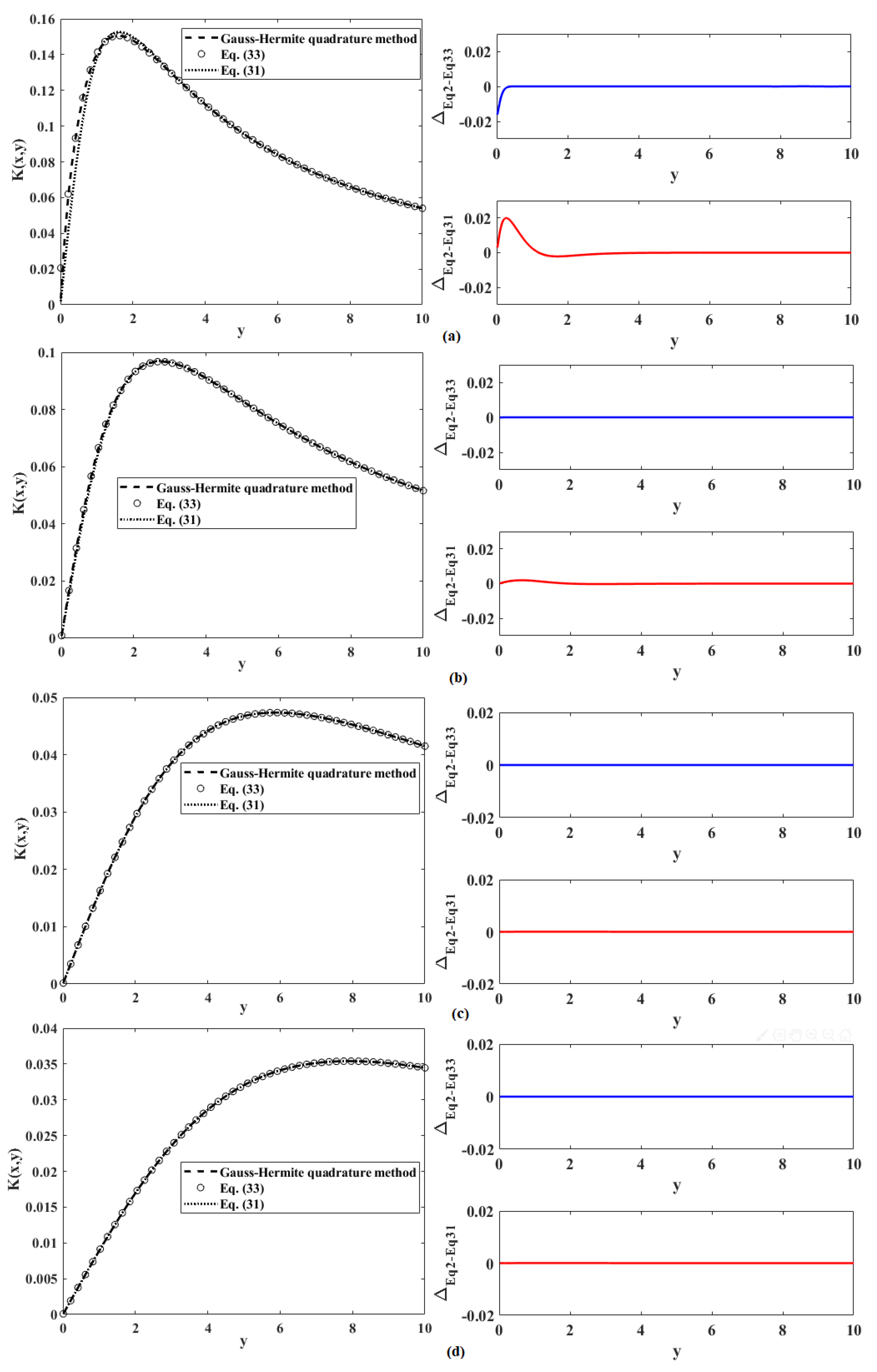
Figure 4 illustrates the evolution of the Voigt function in terms of using our old and new results as well as numerical integration. The difference between our old and new approaches with the numerical integration is plotted to test the degree of agreement. A disagreement between the two analytical expressions for and is observed in Figure 4. However, we can obtain 80% of agreement between our approaches and numerical evaluations from and for all values of . Moreover, we can see that the Voigt profile function reaches its minimum values with the increase in the parameter . On the other hand, we find that the Voigt profile function vanishes at infinity faster with a small value of . The following conclusion can readily be drawn from Figure 4: Equation (33) correctly characterizes the Voigt function in region I. Note that the curves obtained in Figure 4d are identical to the curve plotted in Figure 3a for , which proves the equivalence between Equation (24) and Equations (31) and (33).
The variation of the Voigt function versus for several values of in the second region is plotted in Figure 5. It can observed that the Voigt function can be described by using the two simple approaches (Equations (31) and (33)). For a large value of and , the old formula oscillates because it is expressed as a function of cosine and sine functions, whereas the new approximation remains valid for all values of and large values of . Additionally, as the parameter is increased, the maximum of the peak decreases.
Some plots are depicted in Figure 6 to analyze the behavior of the Voigt function as a function of y and with several values of x. As shown in this figure, for a large value of the maximum of the peak reduces and the profile becomes wider.
Moreover, and by analyzing the comportment of this function from another viewpoint, we notice that for and small values of the curve of the new approach does not coincide with the two other curves that represent the old approximation and the numerical integration. Excellent compatibility between our analytical formulae and the numerical solution using the Gauss–Hermite quadrature method, is obtained from and for all values of
4. Conclusions
The Voigt profile is important place in several fields of physics. In the current investigation, an analytical formula, expressed in terms of a special function, is established. A simple approach is examined to facilitate the manipulation of the Voigt profile. To prove the validity of our new expression, some numerical examples are performed and discussed. The main goal of this work is to present to the readers a simple formula and rapid calculation. These benefits make the study of the Voigt profile more straightforward and convenient. The Voigt profile has an extensive range of applications in different domains such as astrophysics, spectroscopy, and the theory of neutron reactions, among others.
Author Contributions
Investigation, S.C.; writing—review and editing, A.B. All authors contributed equally to this work. All authors have read and agreed to the published version of the manuscript.
Funding
This research received no external funding.
Data Availability Statement
Not applicable.
Acknowledgments
We are grateful to members of our Laboratory for interesting discussions and useful comments. We are also grateful to the anonymous referees for their interesting constructive comments that helped improve the manuscript.
Conflicts of Interest
The authors declare no conflict of interest.
References
- Reiche, F. Uber die emission, absorption and intensitats vertcitung von spektrallicien. Ber. Deutsch. Phys. Ges. 1913, 15, 3–21. [Google Scholar]
- Benedict, W.S.; Herman, R.; Moore, G.E.; Silverman, S. The Strengths, Widths, and Shapes of Infrared Lines: I. General Considerations. Can. J. Phys. 1956, 34, 830–849. [Google Scholar] [CrossRef]
- Hummer, D.G. Non-Coherent Scattering: I. The Redistribution Function with Doppler Broadening. Mon. Not. R. Astron. Soc. 1962, 125, 21–37. [Google Scholar] [CrossRef] [Green Version]
- Armstrong, B. Spectrum line profiles: The Voigt function. J. Quant. Spectrosc. Radiat. Transf. 1967, 7, 61–88. [Google Scholar] [CrossRef]
- Young, C. Calculation of the absorption coefficient for lines with combined Doppler and Lorentz broadening. J. Quant. Spectrosc. Radiat. Transf. 1965, 5, 549–552. [Google Scholar] [CrossRef] [Green Version]
- Yamada, H. Total radiances and equivalent widths of isolated lines with combined Doppler and collision broadened profiles. J. Quant. Spectrosc. Radiat. Transf. 1968, 8, 1463–1473. [Google Scholar] [CrossRef] [Green Version]
- Haubold, H.J.; John, R.W. Spectral line profiles and neutron cross sections: New results concerning the analysis of Voigt functions. Astrophys. Space Sci. 1979, 65, 477–491. [Google Scholar] [CrossRef]
- Whiting, E. An empirical approximation to the Voigt profile. J. Quant. Spectrosc. Radiat. Transf. 1968, 8, 1379–1384. [Google Scholar] [CrossRef]
- Rodgers, C.; Williams, A. Integrated absorption of a spectral line with the Voigt profile. J. Quant. Spectrosc. Radiat. Transf. 1974, 14, 319–323. [Google Scholar] [CrossRef]
- Drayson, S. Rapid computation of the Voigt profile. J. Quant. Spectrosc. Radiat. Transf. 1976, 16, 611–614. [Google Scholar] [CrossRef] [Green Version]
- Minguzzi, P.; Di Lieto, A. Simple Padé approximations for the width of a Voigt profile. J. Mol. Spectrosc. 1985, 109, 388–394. [Google Scholar] [CrossRef]
- Flores-Llamas, H.; Cabral-Prieto, A.; Jiménez-Domínguez, H.; Torres-Valderrama, M. An expression for an approximation of the Voigt profile I. Nucl. Instruments Methods Phys. Res. Sect. A Accel. Spectrometers Detect. Assoc. Equip. 1991, 300, 159–163. [Google Scholar] [CrossRef]
- Teodorescu, C.; Esteva, J.; Karnatak, R.; El Afif, A. An approximation of the Voigt I profile for the fitting of experimental X-ray absorption data. Nucl. Instrum. Methods Phys. Res. Sect. A Accel. Spectrometers Detect. Assoc. Equip. 1994, 345, 141–147. [Google Scholar] [CrossRef]
- Liu, Y.; Lin, J.; Huang, G.; Guo, Y.; Duan, C. Simple empirical analytical approximation to the Voigt profile. J. Opt. Soc. Am. B 2001, 18, 666–672. [Google Scholar] [CrossRef]
- Asfaw, A. A fast method of modeling spectral lines. J. Quant. Spectrosc. Radiat. Transf. 2001, 70, 129–137. [Google Scholar] [CrossRef]
- Letchworth, K.L.; Benner, D.C. Rapid and accurate calculation of the Voigt function. J. Quant. Spectrosc. Radiat. Transf. 2007, 107, 173–192. [Google Scholar] [CrossRef]
- Di Rocco, H.; Cruzado, A. The Voigt Profile as a Sum of a Gaussian and a Lorentzian Functions, when the Weight Coefficient Depends Only on the Widths Ratio. Acta Phys. Pol. A 2012, 122, 666–669. [Google Scholar] [CrossRef]
- Srivastava, H.M.; Miller, E.A. A unified presentation of the Voigt functions. Astrophys. Space Sci. 1987, 135, 111–118. [Google Scholar] [CrossRef]
- Errera, Q.; Vanderauwera, J.; Belafhal, A.; Fayt, A. Absolute Intensities in 16O12C32S: The 2500–3100 cm−1. J. Mol. Spectrosc. 1995, 173, 347–369. [Google Scholar] [CrossRef]
- Belafhal, A. The shape of spectral lines: Widths and equivalent widths of the Voigt profile. Opt. Commun. 2000, 177, 111–118. [Google Scholar] [CrossRef]
- AlOmar, A.S. Accurate Chebyshev Approximations for the Width of the Voigt Profile, Differential Peaks, and Deconvolution of the Lorentzian Width. Optik 2021, 225, 165533. [Google Scholar] [CrossRef]
- Watson, G.N. A Treatise on the Theory of Bessel Functions; Cambridge University Press: Cambridge, UK, 1995. [Google Scholar]
- Gradshteyn, I.S.; Ryzhik, I.M.; Jeffrey, A. Table of Integrals, Series, and Products, 7th ed.; Academic Press: Amsterdam, The Netherlands; Boston, MA, USA, 2007. [Google Scholar]
- Srivastava, H.M.; Karlsson, P.W. Multiple Gaussian Hypergeometric Series; Ellis Horwood: Chichester, UK, 1985. [Google Scholar]
- Singh, D. On Some Representations of Voigt Functions. Ph.D. Thesis, Aligarh Muslim University, Aligarh, India, 2004. [Google Scholar]
- Huang, Q.; Coëtmellec, S.; Duval, F.; Louis, A.; Leblond, H.; Brunel, M. Analytical expressions for diffraction-free beams through an opaque disk. J. Eur. Opt. Soc. Rapid Publ. 2011, 6, 11031–11037. [Google Scholar] [CrossRef] [Green Version]
- Belafhal, A.; Chib, S.; Khannous, F.; Usman, T. Evaluation of integral transforms using special functions with applications to biological tissues. Comput. Appl. Math. 2021, 40, 1–23. [Google Scholar] [CrossRef]
Figure 1.
Different regions used in this paper.

Figure 2.
Illustration of the Voigt function in terms of with

Figure 3.
The generalized Voigt function distribution versus with (a) different values of and (b) contour graph for .
Figure 3.
The generalized Voigt function distribution versus with (a) different values of and (b) contour graph for .

Figure 4.
Illustration of the Voigt function K(x,y) in terms of for different values of : (a) , (b) , (c) , (d) and on the right side, the simulations of the difference between Equation (33), Equation (2) and Equation (31), Equation (2).
Figure 4.
Illustration of the Voigt function K(x,y) in terms of for different values of : (a) , (b) , (c) , (d) and on the right side, the simulations of the difference between Equation (33), Equation (2) and Equation (31), Equation (2).

Figure 5.
Evolution of the Voigt function in terms of for different values of : (a) , (b) , (c) (d) and on the right side, the plots of the subtraction of the Gauss–Hermite result from the result of Equations (31) and (33).
Figure 5.
Evolution of the Voigt function in terms of for different values of : (a) , (b) , (c) (d) and on the right side, the plots of the subtraction of the Gauss–Hermite result from the result of Equations (31) and (33).

Figure 6.
The Voigt function in terms of y for different values of x: (a) , (b) , (c) , (d) and on the right side, the simulations of the difference between Equation (33), Equation (2) and Equation (31), Equation (2) .
Figure 6.
The Voigt function in terms of y for different values of x: (a) , (b) , (c) , (d) and on the right side, the simulations of the difference between Equation (33), Equation (2) and Equation (31), Equation (2) .


Table 1.
Table of abscissas and weight factors for Gauss–Hermite integration.
| 1 | 0.2453407083009 | (−1) 4.622436696006 |
| 2 | 0.7374737285454 | (−1) 2.866755053628 |
| 3 | 1.2340762153953 | (−1) 1.090172060200 |
| 4 | 1.7385377121166 | (−2) 2.481052088746 |
| 5 | 2.2549740020893 | (−3) 3.243773342238 |
| 6 | 2.7888060584281 | (−4) 2.283386360163 |
| 7 | 3.3478545673832 | (−6) 7.802556478532 |
| 8 | 3.9447640401156 | (−7) 1.086069370769 |
| 9 | 4.6036824495507 | (−10) 4.399340992273 |
| 10 | 5.3874808900112 | (−13) 2.229393645534 |
Publisher’s Note: MDPI stays neutral with regard to jurisdictional claims in published maps and institutional affiliations. |
© 2022 by the authors. Licensee MDPI, Basel, Switzerland. This article is an open access article distributed under the terms and conditions of the Creative Commons Attribution (CC BY) license (https://creativecommons.org/licenses/by/4.0/).
Share and Cite
MDPI and ACS Style
Chib, S.; Belafhal, A. Simple Analytical Expression of the Voigt Profile. Quantum Rep. 2022, 4, 36-46. https://doi.org/10.3390/quantum4010004
AMA Style
Chib S, Belafhal A. Simple Analytical Expression of the Voigt Profile. Quantum Reports. 2022; 4(1):36-46. https://doi.org/10.3390/quantum4010004
Chicago/Turabian StyleChib, Salma, and Abdelmajid Belafhal. 2022. "Simple Analytical Expression of the Voigt Profile" Quantum Reports 4, no. 1: 36-46. https://doi.org/10.3390/quantum4010004