1. Introduction
Over the last few years, a variety of driving assistance systems have become widespread. These functions make driving safer and more comfortable, but the presence of a human driver is still essential. To take the next step, a much higher level of autonomous capability is needed, allowing the vehicle to operate in a greater number of situations without the intervention of the driver. To this end, accurately controlling the vehicle in any driving situation is essential.
In a decoupled control architecture, which is commonly used in the literature, lateral control aims to guide the vehicle to stay on the path without losing stability or impairing passenger comfort, regardless of whether the road has sharp curves or the vehicle is traveling at high or low speeds. This problem has been addressed using different approaches, one of which involves improving the available model of the vehicle in order to better tune a model-based regulator, which is a very complex task due to the nonlinear and variant characteristics of the system. Some authors have attempted to design controllers for different speed-specific driving situations and provide a fitting law between the different parameters or outputs of the controllers. To avoid the problems induced by complex system identification, model-independent strategies are gaining interest.
Speed-Adaptive Model-Free Control (SAMFC) [
1] is a path-tracking control strategy for autonomous vehicles framed within the Model-Free Control (MFC) paradigm [
2]. It is based on the adaptation of one of the key parameters of MFC as a function of driving speed, allowing the vehicle to cope with a variety of situations without having to re-tune the controller for any of them. In this paper, SAMFC is analyzed in a more formal and extensive way. To thoroughly evaluate the potential of this strategy in comparison with a standard MFC controller, metrics of tracking quality, stability of the feedback system, and passenger comfort are defined. A noniterative design procedure is proposed to obtain control configurations that meet specific time-response and frequency-response specifications. Therefore, the main contribution of this work lies in the introduction, analysis, and design procedure of an easy-to-implement variation of MFC, which has proven to be very effective for lateral control of automated vehicles.
The rest of this paper is structured as follows.
Section 2 presents a brief review of lateral control strategies in the literature, focusing on model-independent approaches. A theoretical introduction to Model-Free Control is presented in
Section 3.
Section 4 introduces the proposed Speed-Adaptive Model-Free Control strategy and provides an analysis of its usefulness, as well as a design procedure. The results of the simulation and real-world tests are presented in
Section 5. Finally,
Section 6 presents some concluding remarks and references.
2. State-of-the-Art Literature
Lateral control of autonomous vehicles is studied from different approaches [
3], most of which are based on a somewhat realistic model of the vehicle, with the single-track model being the most popular [
4]. The success of this vehicle dynamics representation lies in its linear nature, which assumes a constant longitudinal velocity. Some real applications show that this simplification may be inappropriate for providing accurate lateral control in every driving circumstance. To overcome these limitations, different model-based feedback strategies have been proposed in the last few years. Ref. [
5] applied the single-track model to fit two PID (Proportional-Integral-Derivative) regulators, one for low and one for high speeds. Ref. [
6] used the model to synthesize a robust LQR (Linear Quadratic Regulator). Ref. [
7] applied the Lyapunov theory to obtain an asymptotically stable regulator on an extended model. Another approach is gain scheduling, which was applied in [
8] to control an electric vehicle. Alternatively, Model Predictive Control (MPC) strategies have also been developed and evaluated in real cars. Some of these strategies rely on a more complex model [
9], whereas others focus on jointly solving the path-planning and control problems [
10]. However, they are mainly tested in specific driving situations. In [
11], a cascade MPC-PD structure was applied in a shared control architecture to perform an overtaking maneuver.
Real vehicles have complex dynamics that vary with speed and steering angle and have strong nonlinearities in the tire–ground interface, as well as the steering and suspension systems. Additionally, there are couplings between lateral and longitudinal dynamics, as well as variability in parameters that are already difficult to characterize such as wheel stiffness or inertia, which depends on the mass distribution within the vehicle. Consequently, it is extremely hard to find a realistic model that covers a wide range of driving situations. As a result, control strategies that do not rely on a vehicle dynamic model have attracted attention from the research community.
Fuzzy control is a good example of a model-free technique. It enables the control of nonlinear systems, absorbs some of the variability in the system parameters, and results in a formulation that is intuitive but difficult to tune optimally over a wide working range. Two fuzzy regulators were integrated and validated in traffic-based driving environments [
12]. Other works [
13,
14] have confirmed the capabilities of fuzzy lateral control for autonomous vehicles. Another approach is pure pursuit control [
15], which is based on a vehicle kinematic model. Although it behaves reasonably well at low speeds, its performance degrades when high velocities or accelerations are requested.
The MFC framework mentioned in the introduction has been successfully applied in vehicle longitudinal control applications [
16] and in lateral control for low-speed Automated Guided Vehicles [
17], as well as in other applications [
18,
19]. Alternatively, in [
20], the flatness theory [
21], which enables the identification of differentially flat outputs for nonlinear systems, was applied to implement the lateral control of a vehicle together with a model-free feedback controller. This approach exhibited very good performance in simulation. However, its deployment in real vehicles is not straightforward, as it requires measurements that cannot be obtained using commercial sensors. A special case is Ultra-Local Model Predictive Control (ULMPC) [
22], which is a unique combination of model-free and model-based approaches. This approach involves the application of an MPC regulator that uses a state representation of the ultra-local model proposed in MFC. However, the computational power required by ULMPC, although lower than that of MPC, is higher than that of MFC, as a real-time solver is still needed.
Alternatively, the authors of [
23] proposed an adaptation mechanism for MFC and applied it on a scale car. However, the resulting adaptation dynamic is too slow for automated vehicles driving on real roads. Other examples of adaptation mechanisms for MFC can be found in the literature. The authors of [
24] proposed an adaptation law for
based on the knowledge of the nominal model of the system. Similarly, the authors of [
25] proposed an MFC-modified control structure and an adaptation law for
based on a Lyapunov function. Additionally, the authors of [
26] proposed an adaptation law for
based on least squares estimation and applied it to a seven-degree-of-freedom upper-limb exoskeleton.
3. Model-Free Control Principles
Model-Free Control [
2] is a newly developed control framework for SISO systems, which has demonstrated its performance across a wide variety of applications, as discussed in
Section 2. This framework involves reducing the system’s dynamics, which can be nonlinear, time-varying, or complex to identify, using a simple model that is updated online known as the ultra-local model (
1).
A demonstration of this approximation is as follows. Assume that the dynamics of the considered SISO system can be defined by the algebraic differential equation
, which establishes a relationship between its input
u and output
y (along with their derivatives). Additionally, consider
n as a non-negative integer such that
, therefore
can be rewritten locally as
. This equation yields the ultra-local model:
in which the relationship between the input
u and the nth derivative of the output
y of the system is considered linear, with a constant ratio
that is a design parameter. This linear relationship is fitted by a variable
F that absorbs model errors and system disturbances.
Further, the feedback control is defined to reduce modeling and tracking errors, resulting in an
intelligent controller:
where
u is the control action,
is the nth derivative of the output reference,
e is the tracking error, and
is a classical controller expression.
Among the intelligent controllers, the iPD controller is the most widely used:
where
and
are the control parameters.
The term F has to be updated continuously and, therefore, must be estimated in real time using an estimator .
Implementation of Model-Free Controllers
The MFC controllers implemented in this paper are second-order iPDs (
); therefore, (
3) yields the control action
:
where
is the current instant,
is the lateral deviation of the vehicle,
e is the tracking error, and
is the filtered estimation of the tracking error derivative.
In order to estimate
F, various estimators can be considered, but in the remainder of this paper, a simple one is applied due to its high performance and low computational time. The estimator assumes that
F remains constant between consecutive instants, allowing it to be estimated from previous control actions based on (
1) as follows:
where
is the estimation of the nth derivative of
y. This estimation is obtained by applying the following filtered derivative operator
n times to the output of the system:
where
is the sample time and
C is the filtering parameter, which is experimentally set at
so that the measurement noise is reduced.
5. Results
In this section, a noniterative design procedure is applied (
Section 5.4) using the simplified lateral dynamics model of the vehicle described in
Section 4.2.2. The control configurations obtained are evaluated using the extended vehicle simulator described in
Section 5.1, along with three metrics (defined in
Section 5.3), across a wide range of driving contexts (described in
Section 5.2). The performance of the resulting control configurations is compared in simulations to that of the parameter sets obtained with the iterative design procedure using the extended vehicle simulator (
Section 5.7). To confirm the potential of the proposed control structure and design method, several experimental trials are conducted in an automated prototype, and the results are reported in
Section 5.8.
5.1. Vehicle Extended Model
In order to ensure a faithful representation of the experimental platform outlined in [
28], simulation tests were carried out using the same vehicle model described in [
1]. The dynamic model chosen for this purpose was a 14-degree-of-freedom system (6 for the vehicle body motion—longitudinal, lateral, vertical, roll, pitch, and yaw—and 8 for the wheels—vertical motion and spin of each wheel).
The powertrain model consisted of three components: (i) the engine, represented by its torque map, which was determined using the experimental platform data; (ii) the gearbox, which incorporates the same drive ratios and gear-shift logic as the actual vehicle; and (iii) the resistive torques from the braking system, wind forces acting longitudinally, and gravitational forces. The tire behavior was reproduced using the Pacejka tire model [
29].
In addition to the electric power-assisted steering system already in place in the vehicle, an external actuation system was incorporated following the guidelines of [
30]. To ensure the accuracy of the model, essential parameters such as inertia and backlash were measured or identified through extensive field tests. Moreover, the noise produced by the localization system of the experimental platform was characterized and included in the simulation model.
It should be noted that this model does not take into account climate conditions such as the wind effect or the state of the asphalt.
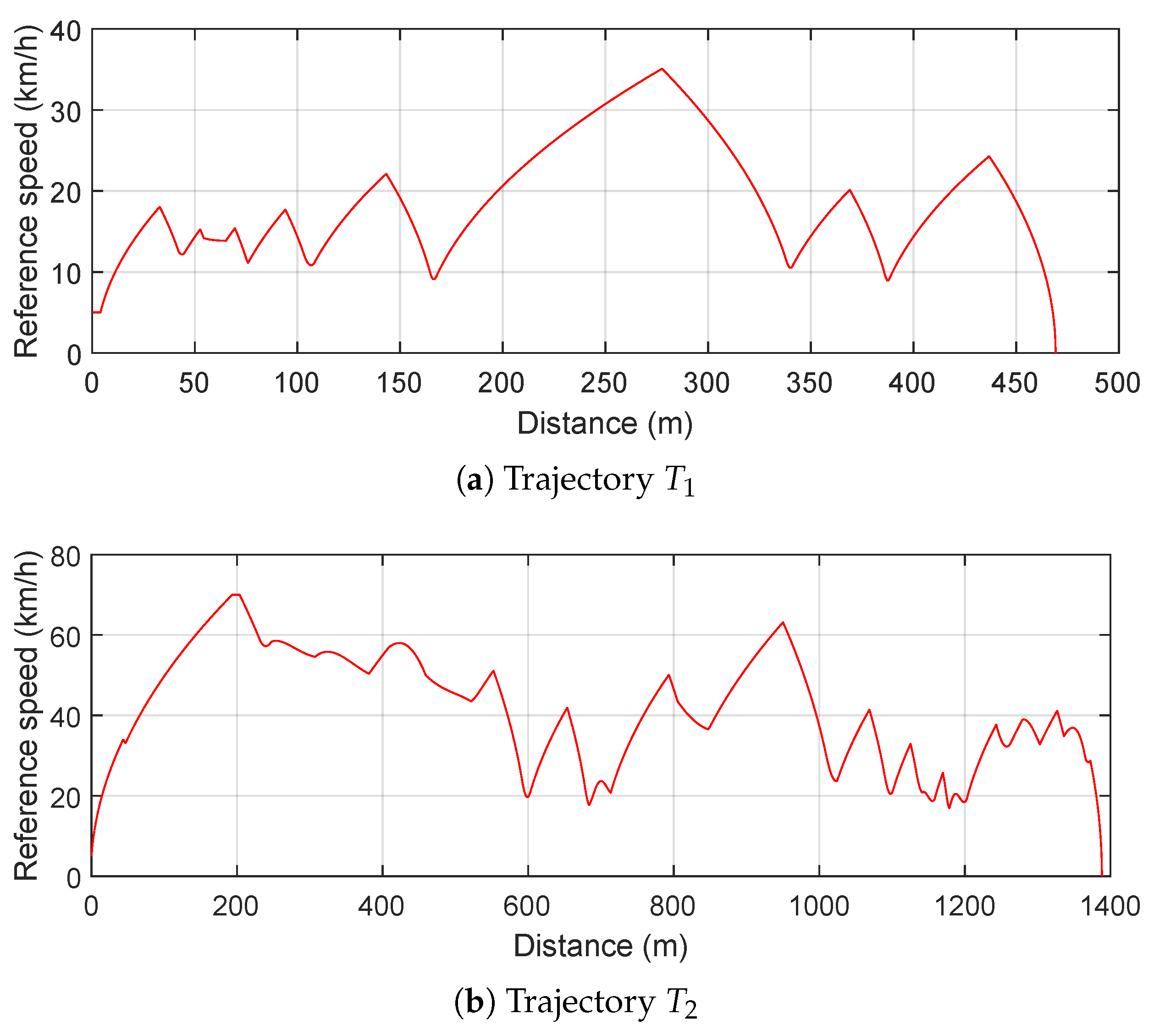
5.2. Benchmark Description
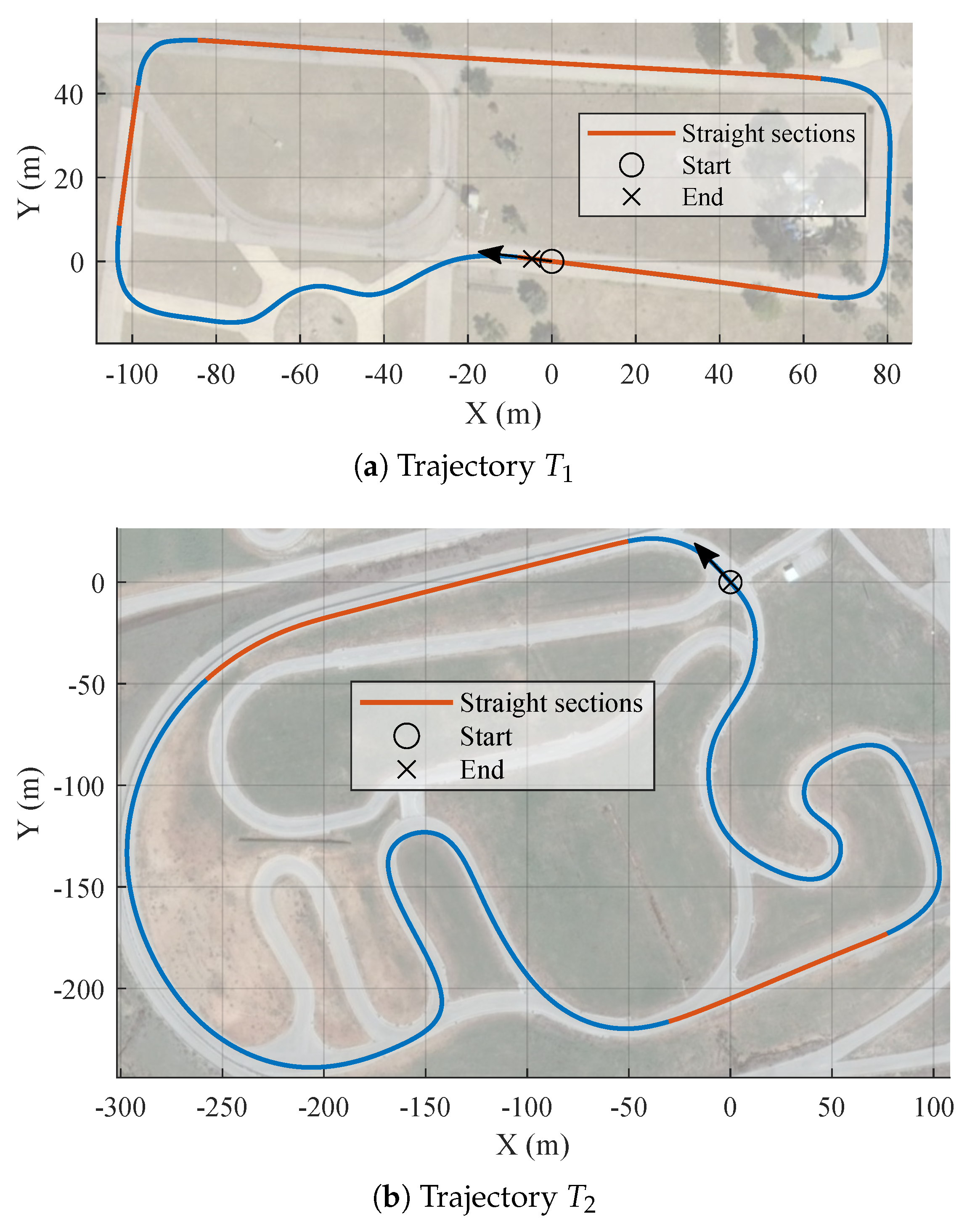
Figure 3 shows an aerial view of the two circuits used in the simulation and real-world tests. The trajectories
and
were designed to cover a wide range of realistic driving scenarios, including straight sections, curves of different natures, varying maximum speeds, and longitudinal and lateral accelerations.
was designed as an urban scenario, including intersections and a roundabout, whereas
was designed to emulate a regional road with higher-speed straight stretches and both slow and fast curves.
To ensure the continuity of the curvature across the paths, they were defined by a cubic B-spline, which ensured
continuity. Then, to generate the reference trajectories, speed profiles were computed for each path by applying the method for acceleration-limited speed planning proposed in [
31]. The maximum speed and accelerations used to calculate the speed profile are shown in
Table 2. The resulting speed profiles obtained are illustrated in
Figure 4.
5.3. Metrics Description
In this section, the metrics used to measure the performance of the controllers are analyzed in terms of tracking quality and control action. It should be noted that the metrics used in this work were introduced in [
1].
The integral absolute lateral error (IAE) was used to assess tracking quality. However, to the best of the authors’ knowledge, there has been no consensus on the metrics used to assess vehicle stability and passenger comfort (see Section 5.3 of [
32] for a review of the different metrics used in the state-of-the-art literature). It was experimentally found that the classical IAU (Integral of the Absolute Value of the Control Action) and IAUD (Integral of the Absolute Value of the Derivative of the Control Action) were too simplistic to properly analyze the control action dynamics and they do not represent vehicle stability and passenger comfort. Therefore, an analysis of the frequency spectrum of the feedback control action was used to define two different performance indicators:
- 1.
: this metric quantifies the low-frequency oscillations of the control action, which can lead to vehicle instability.
- 2.
: this variable quantifies the high-frequency oscillations of the control action, which can cause discomfort to the vehicle occupants.
The values of both metrics, and , were computed in two separated frequency bands: (1.1–4 Hz) and (4–10 Hz), respectively. It should be noted that a control frequency of 20 Hz was assumed in this work. A high-pass filter was initially applied to the feedback control action to remove unwanted spectral power values at low frequencies. The cutoff frequencies of these filters were 0.5 and 4 Hz for and , respectively. Then, the spectrum was calculated by applying the short-time Fourier transform with 5-s overlapping sections.
The value of
was finally calculated as the mean of the maximum power spectrum at each section, considering a scale factor and a threshold to balance the order of magnitude of both metrics:
where
n is the amount of 5-s sections,
is the spectrum power of band
in section
i,
is a scale factor (
), and
is a threshold in dB (
dB).
The high sensitivity of
can lead to incorrect metric values in curves due to its low-frequency spectrum. Therefore, only straight and long sections, where the path curvature is below
m
and the vehicle drives for more than 5 s (considering the speed profile of each trajectory), were considered. The straight sections for each test trajectory are highlighted in orange in
Figure 3.
The procedure used to obtain was also applied to calculate . However, instead of using the mean value, the maximum power among all sections was assigned to this metric, with a scale factor of and the same threshold of dB. This particular choice was motivated by the low equivalence observed in the experimental tests between the intended interpretation of this metric and the value obtained when using the mean value. The experimental tests showed that when the mean value of all sections was used, the isolated occurrence of high frequencies caused the value of the metric to be low, even though the oscillations caused discomfort. When the maximum value within each section was used, the metric correctly indicated the presence of oscillations that caused discomfort. However, when the maximum power was considered, controllers that exhibited high-frequency oscillations in any section of the test trajectory had high values of .
To summarize, IAE was the chosen indicator of reference tracking quality, was used to measure the (in)stability margin of the controller, and was used to measure passenger discomfort.
To illustrate the magnitude of the performance metrics, it was experimentally observed that an IAE greater than 0.35 m implies poor path tracking in the curves, an greater than 0.25 implies the possibility of system instability when the speed is high, and an greater than 0.7 indicates a loss of passenger comfort.
5.4. Standard MFC Parameter Design
The design procedure to obtain SAMFC configurations, which was introduced in
Section 4.3, relies on control configurations of standard MFC controllers. Several approximations to the MFC controller design problem have been proposed [
33,
34,
35]. In [
33], an MFC tuning procedure using the least squares method was proposed. In [
34], an
adaptation law for autonomous vehicle applications and a design method based on a quadratic cost index and a decision tree were proposed.
In this paper, the standard MFC controller configurations were obtained by applying the design procedure introduced in [
35]. This method allows to obtain MFC controller configurations that meet user-defined time-response and frequency-response specifications. It is based on the relationship between MFC controllers and Three-Term Controllers, as well as the root-counting and phase-unwrapping formulas from [
36].
It was proven in [
35] that a three-term controller in its Z-transform representation
and a second-order iPD controller in its Z-transform representation
are related by
when the three-term controller (
13) is applied to
, with
being the system to be controlled.
With this relationship, the design methods for three-term controllers collated in [
36] can be applied. These procedures allow the designer to obtain the stabilizing set of the controller for a given system, i.e., the control parameter configurations that make the closed-loop stable. By using the stabilizing set for a three-term controller and (
15), the stabilizing set for an MFC controller can be obtained. Finally, the design method described in
Section 4.3 can be applied.
5.5. Feedforward Control
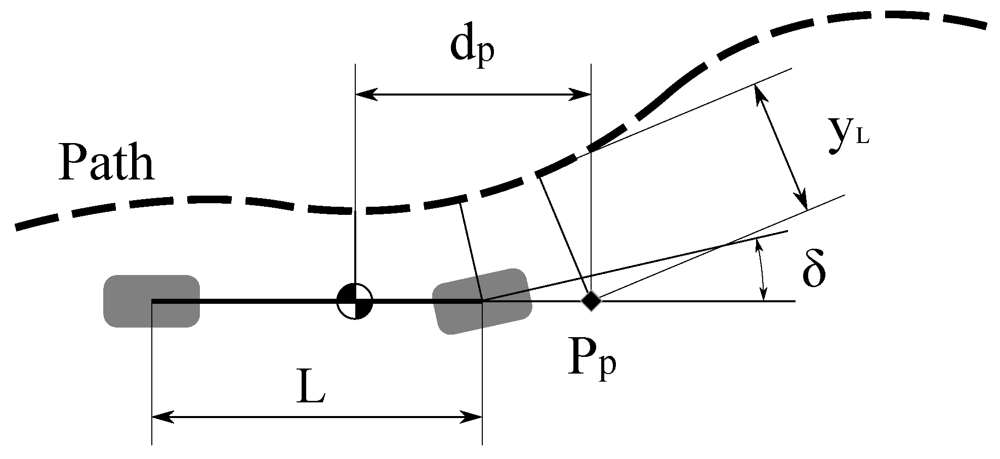
A feedforward term
was added to the feedback control action
to compensate the path curvature. This term was designed to lighten the load on the feedback controller when the vehicle enters a curved section. Then, the complete steering wheel control action can be expressed as
The feedforward term was applied in [
1,
12] and depends on a kinematic model of the vehicle and the curvature of the path, as shown in
Figure 5. In
Figure 5,
is the lateral deviation at the preview point
, and
is the preview distance from the vehicle’s CoG. It should be noted that the speed-based variable preview distance was considered to obtain the feedback control action such that
, where
is the minimum preview distance,
is the preview time, and
and
are tunable parameters considered for the implemented controllers.
Given these considerations, the feedforward controller is defined as
where the feedforward control action is normalized (
),
L is the wheelbase,
is the path curvature,
is the steering ratio, and
is the maximum steering angle.
5.6. Control Configurations Evaluated
Two feedback control strategies were evaluated: the iPD (MFC) from Equations (
4)–(
6) and the Speed-Adaptive iPD (SAMFC) from Equations (
4)–(
7). Using these strategies, two evaluations were conducted: (i) to test the suitability of SAMFC, an iterative design procedure was applied to obtain the (SA)MFC controller configurations that optimized the performance metrics defined in
Section 5.3, and (ii) to evaluate the results of the proposed design procedure (
Section 5.4), it was applied to the vehicle model (
10) to obtain different (SA)MFC controller configurations that were compared to those of the iterative procedure.
The tunable parameters of the evaluated strategies are
MFC: , , , , and
SAMFC: , , , , , , and
5.6.1. Iteratively Designed Configurations
An iterative design procedure was applied to obtain an iPD controller configuration and an SAMFC controller configuration. These configurations minimized the performance metrics defined in
Section 5.3 when evaluated on the benchmark trajectories (
Section 5.2) using the extended vehicle simulator (
Section 5.1). This design procedure was introduced in [
1]. The control configurations obtained are shown in
Table 3.
5.6.2. Noniteratively Designed Configurations
It should be noted that, as the design method proposed in this work (
Section 5.4) considers a dynamic vehicle model without a preview point, the values of
and
are assumed to be zero (
).
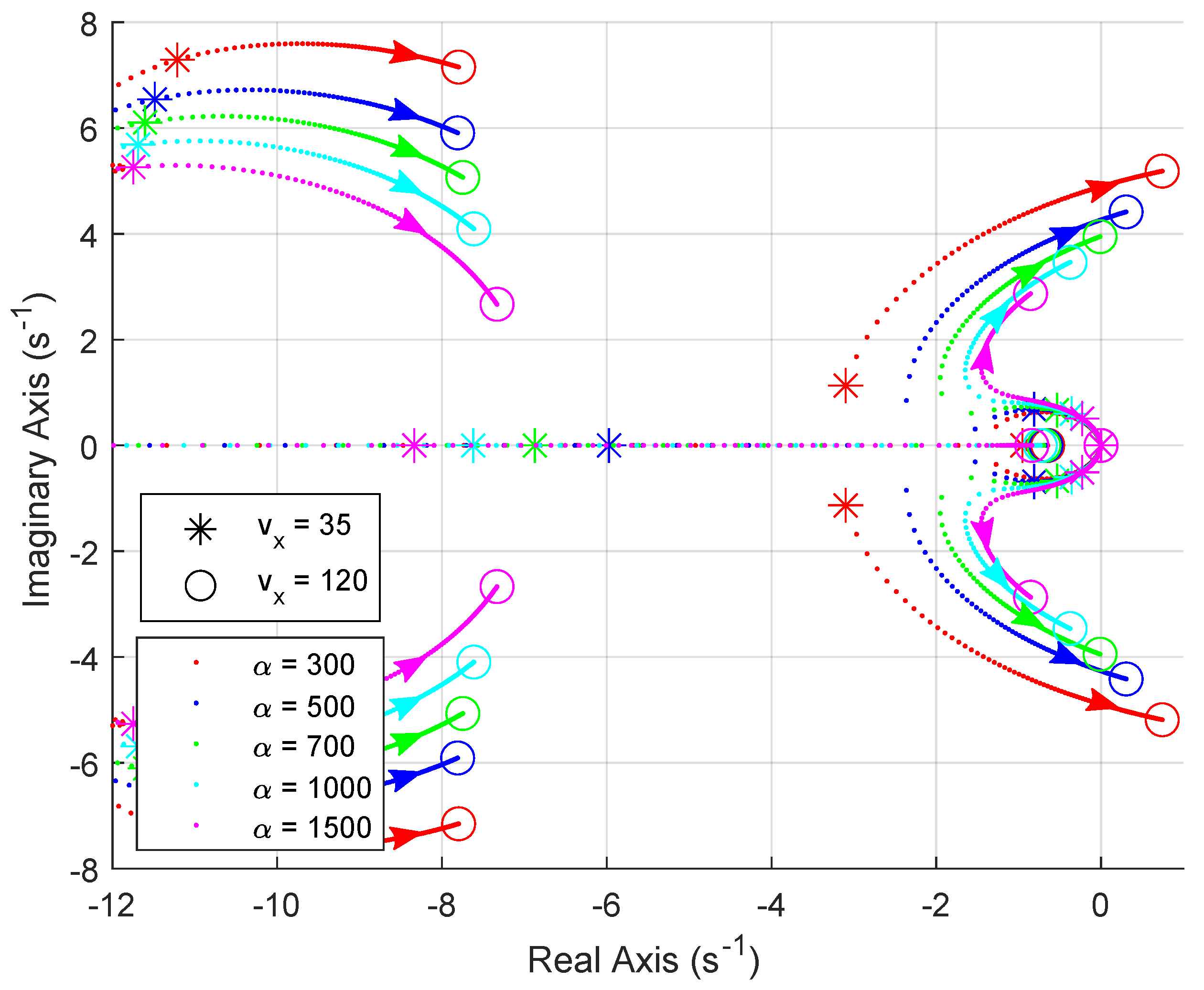
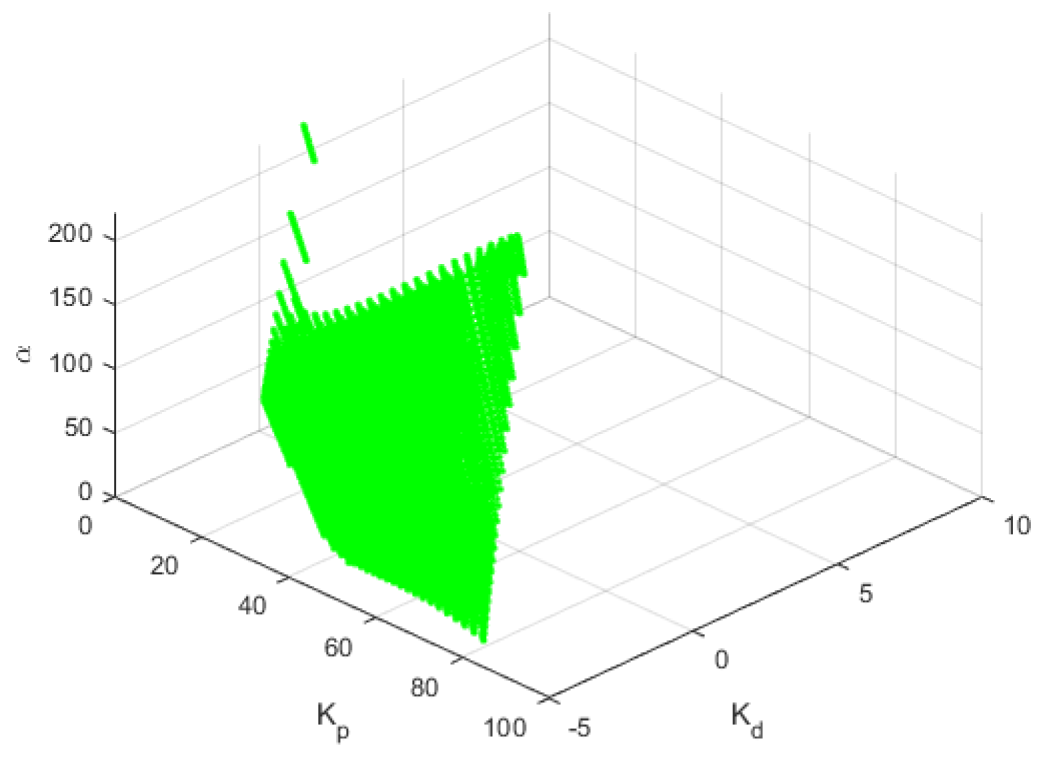
By applying the method described in
Section 5.4 to the vehicle model (
10), an iPD stabilizing set was obtained for high speeds (70 km/h). The stabilizing set obtained is shown in
Figure 6. From this set, any configuration can be chosen by the designer. In this work, the configuration that could satisfy the most demanding frequency-response restrictions—namely, Gain Margin (GM) and Phase Margin (PM)—was chosen. It should be noted that the number of available configurations depends on the discretization step applied in the design procedure.
In order to obtain the configuration for low longitudinal speeds (20 km/h), the frequency response of the closed-loop system was evaluated at
km/h. The parameter
was adjusted by reducing its value (i.e., the controller was made more aggressive) until the margins at 20 km/h were similar to those of the high-speed configuration at 70 km/h, as described in
Section 4.3. It should be noted that, although this part of the design procedure is iterative, only one parameter needs to be tuned, which can be done using information from the nominal model of the system.
Table 4 shows the selected configurations and their nominal frequency-response specifications. Using the procedure described in
Section 4.3, an SAMFC controller was obtained from both low- and high-speed MFC configurations, as shown in
Table 5.
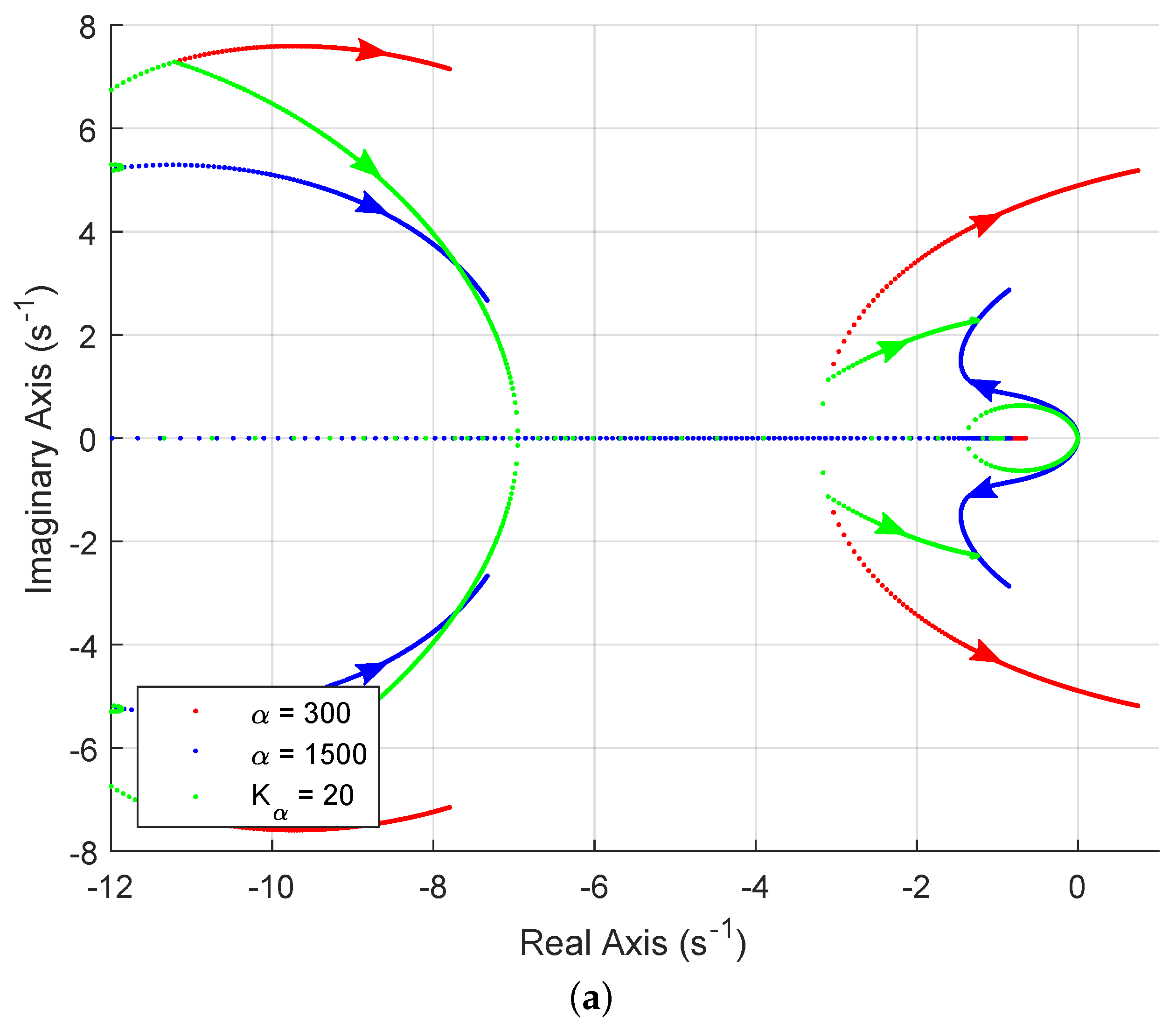
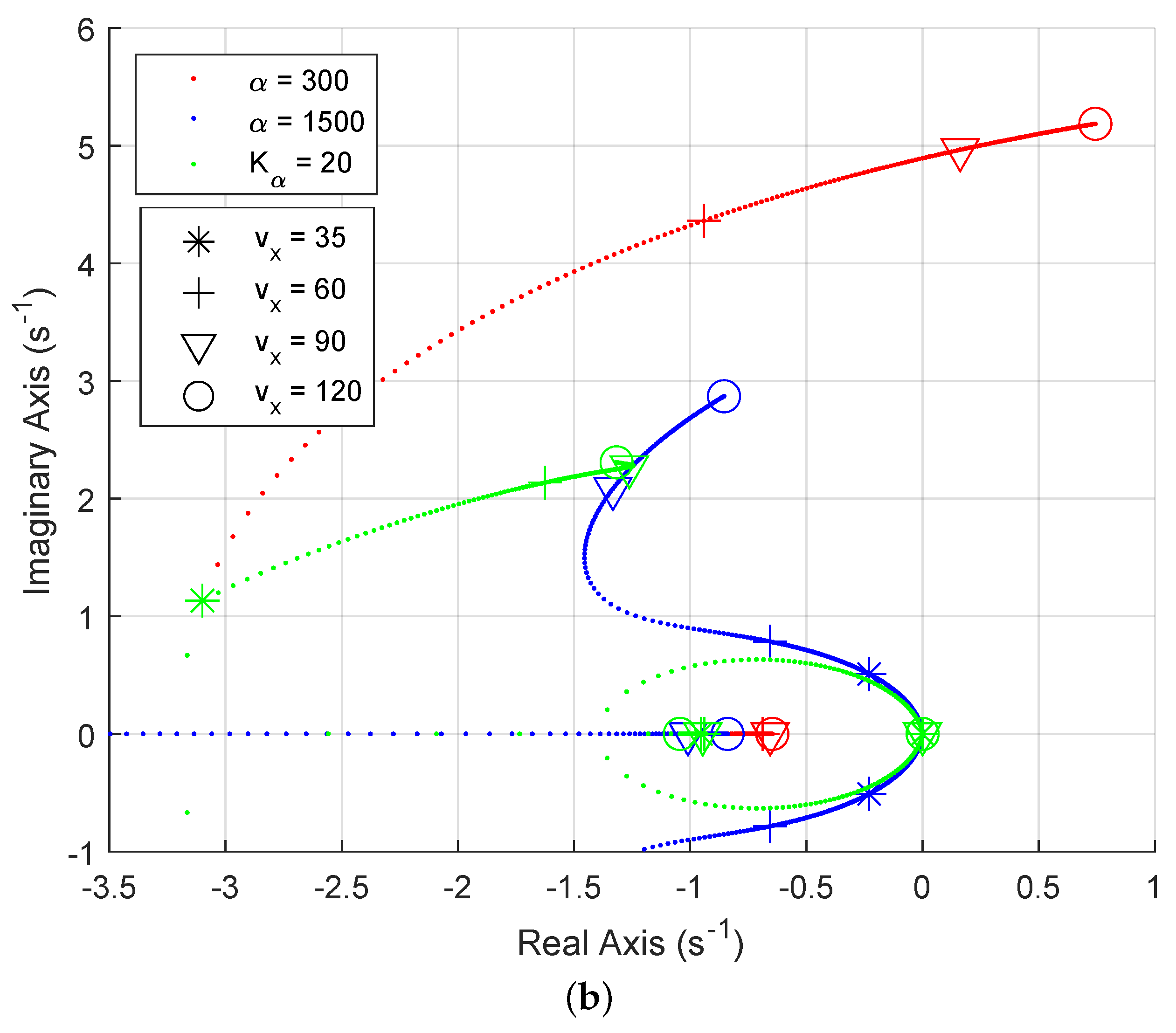
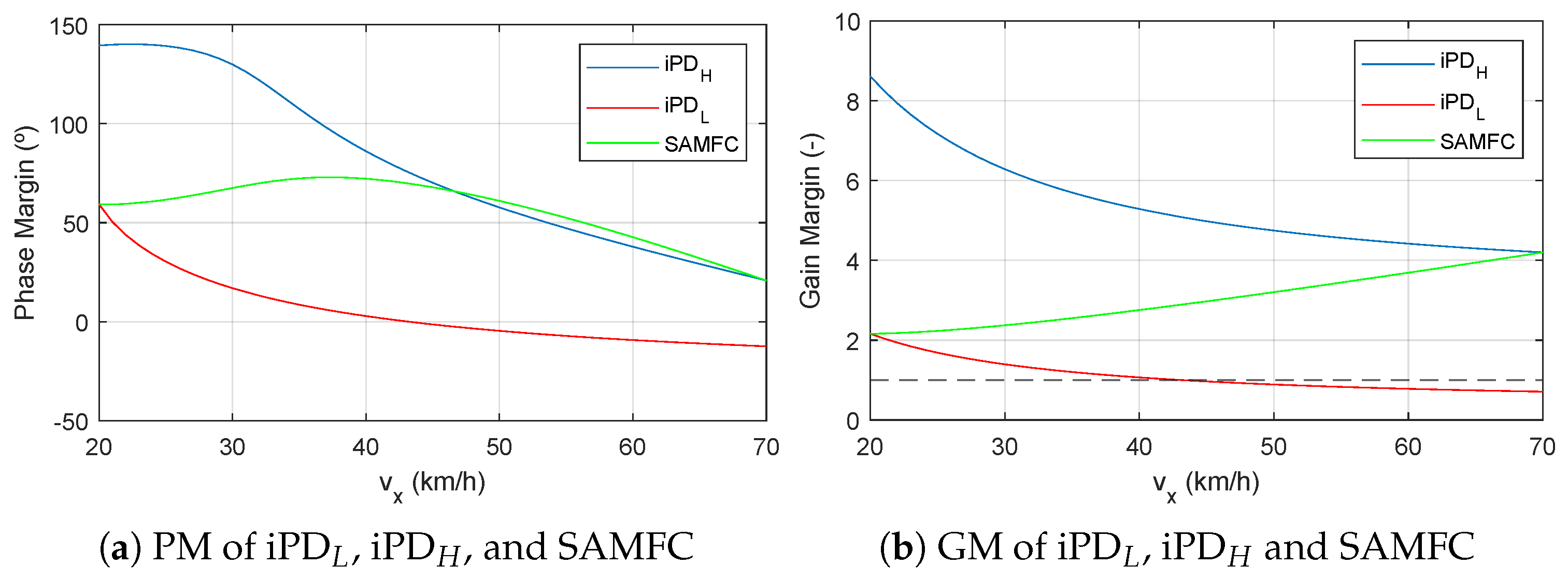
The frequency-response specifications of the SAMFC controller designed for varying speeds are shown in
Figure 7, where the dotted line in
Figure 7b represents GM
. It can be observed that the SAMFC controller maintained greater consistency in both frequency-response specifications across the studied speed range than the MFC controllers used to design it. This characteristic indicates that the expected response will be uniform across different driving scenarios.
5.7. Simulation Results
In order to evaluate the performance of the five controllers obtained from both design procedures, simulations were conducted using the extended vehicle model (
Section 5.1) on the two benchmark trajectories (
Section 5.2). These trajectories cover a large number of driving scenarios and have different driving dynamics. The performance of the controllers was evaluated using the performance metrics described in
Section 5.3. The results are presented in
Table 6.
On the one hand, the iteratively designed SAMFC (SAMFC
) controller was able to improve the tracking quality metric (IAE) compared to the iteratively designed iPD (iPD
) controller while maintaining the stability and passenger comfort metrics (
and
) within an acceptable range. On the other hand, the tracking quality of the noniteratively designed MFC controllers (iPD
and iPD
) was compromised when simulated on trajectories with different dynamic constraints from those for which they were originally designed. This effect was particularly pronounced in the case of iPD
, where instability was observed in
, as seen in
Figure 7a,b. The noniteratively designed SAMFC controller exhibited better tracking quality than the MFC controllers from which it was originally obtained; however, there was a trade-off in passenger comfort (
).
The results in
Table 6 show that (i) the SAMFC controller was able to improve the strategy of the standard MFC controller for the path-tracking control of an autonomous vehicle, and (ii) the proposed noniterative design procedure allowed to obtain competitive configurations with the information from a simplified vehicle model while being less computationally expensive than the iterative procedure.
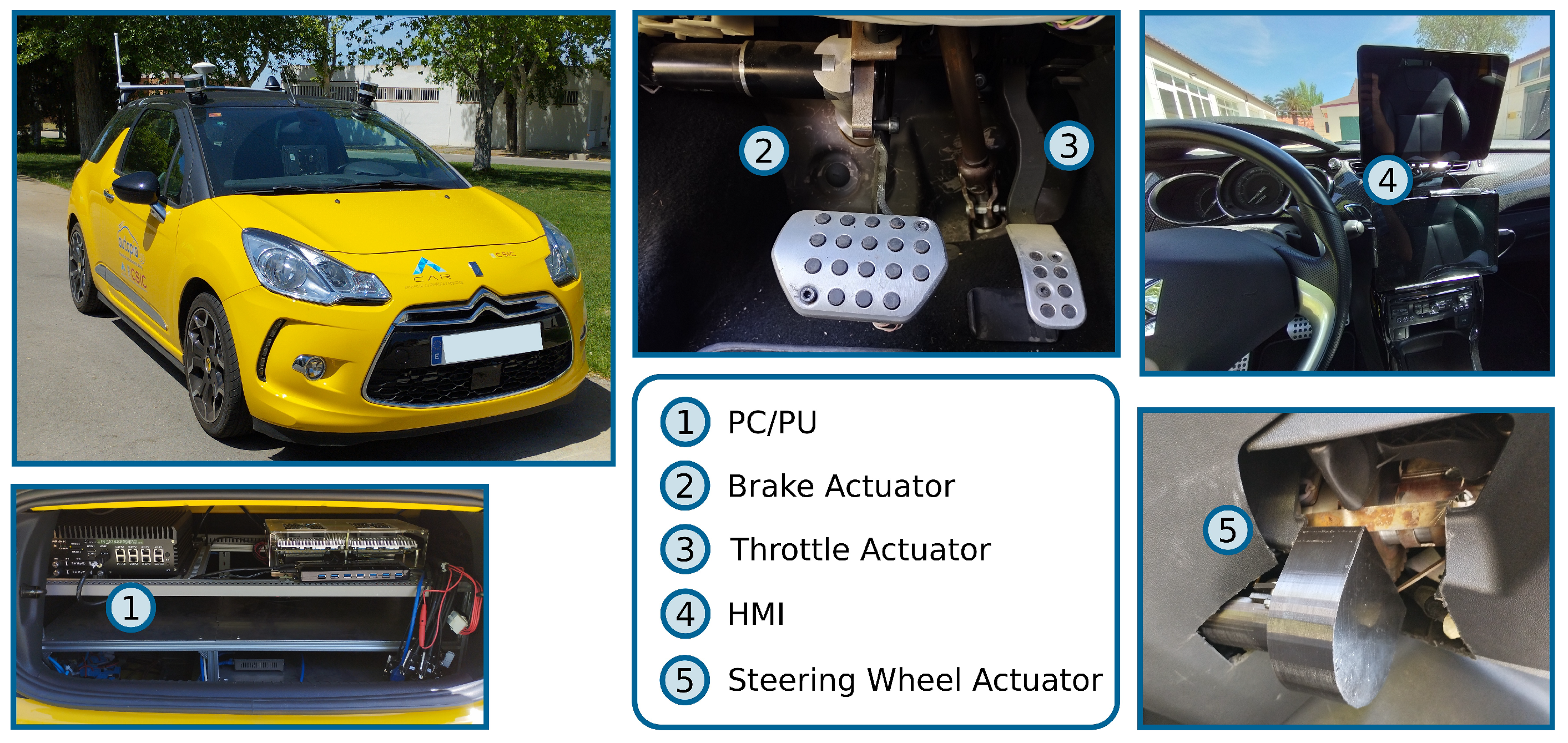
5.8. Experimental Results
The vehicle used in the experiments was a Citroën DS3, which included hardware modifications for the automated control of the throttle, brake, gearbox, and steering systems (see
Figure 8).
The localization of the vehicle relied on an RTK-DGPS receiver and onboard sensors to measure the vehicle’s speed, accelerations, and yaw rate. An onboard computer with an Intel Core i7-8700T and 8Gb RAM was used to run the control algorithms. The vehicle was also equipped with exteroceptive sensors to perceive the environment [
28].
To test the performance of the controllers in real environments, the controllers presented in
Table 3,
Table 4 and
Table 5 were implemented on the experimental platform and tested on test tracks
and
. Although the tracking quality of the controllers in the real-world tests was slightly worse than in the simulations, the results (see
Table 7) showed that the SAMFC controllers achieved better tracking quality than the MFC controllers. It should also be noted that the passenger comfort metric
was generally affected in the real-world tests due to differences between the vehicle extended model (
Section 5.1) and the experimental platform.
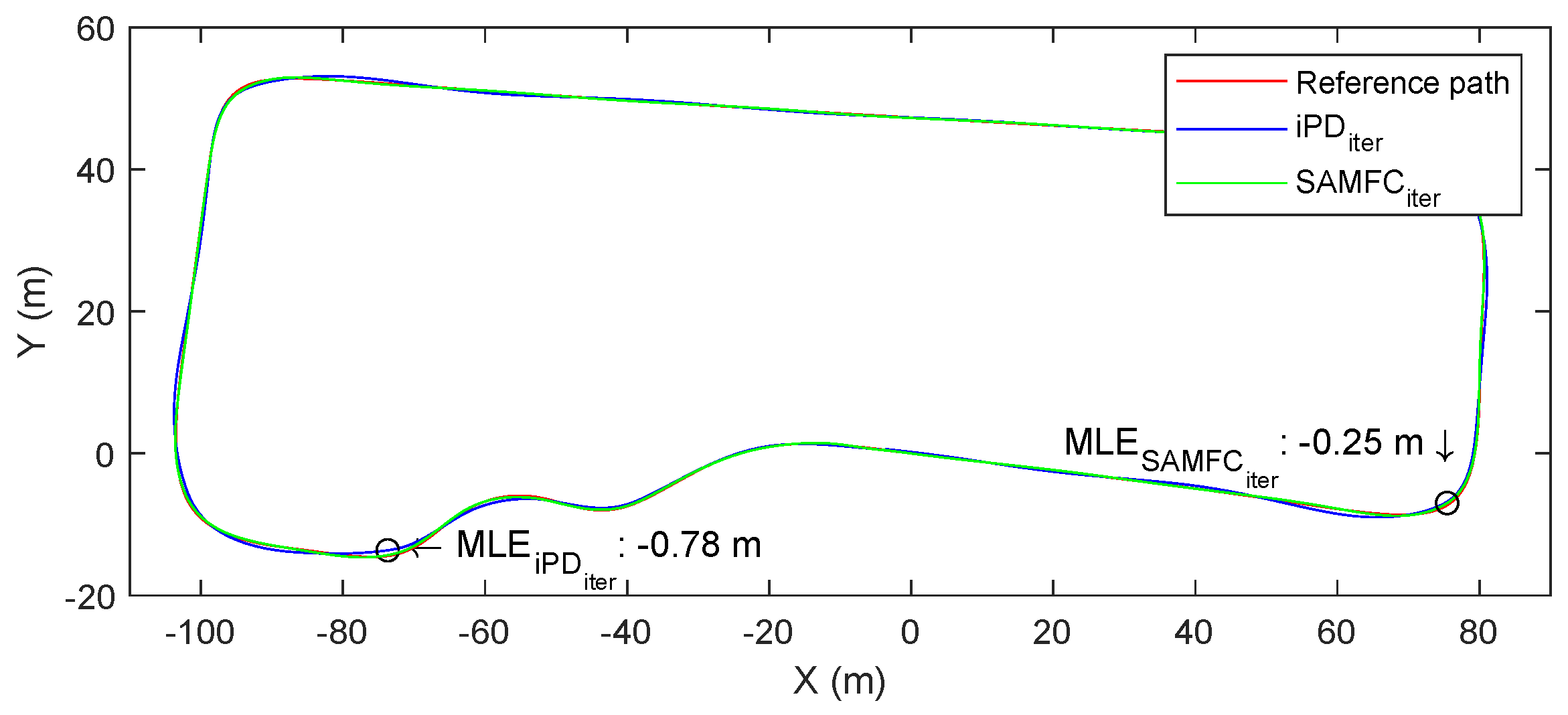
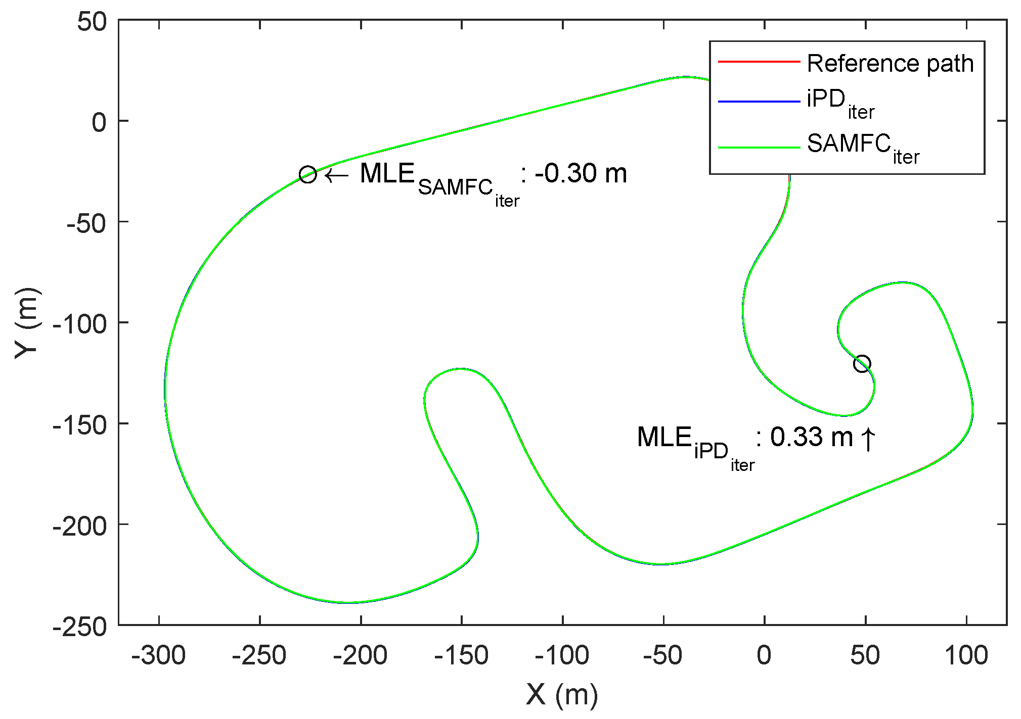
Figure 9 shows the performance of the iteratively designed MFC and SAMFC controllers and
Figure 10 shows the behavior of the noniteratively designed SAMFC controller, as well as the MFC controllers from which it was originally designed, on the benchmark trajectory
. As can be seen, the SAMFC controllers exhibited a lower Maximum Lateral Error (MLE) than the respective standard MFC controllers.
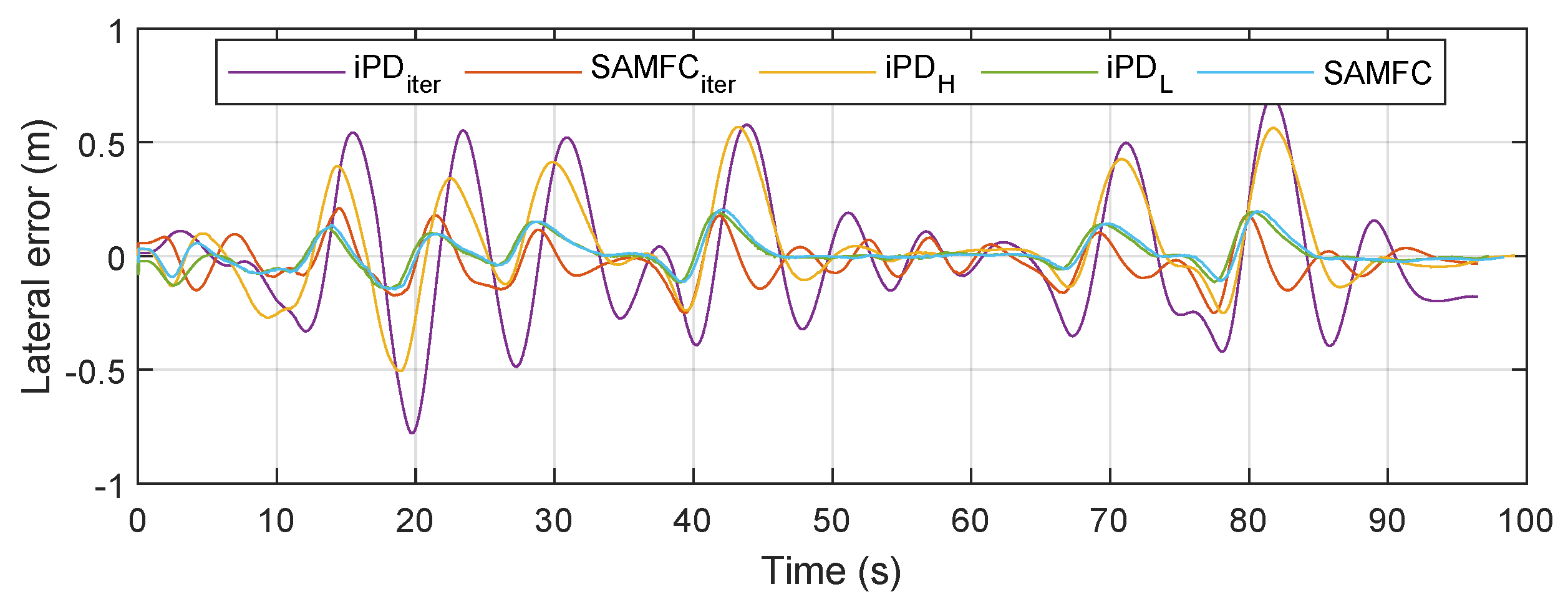
Figure 11 shows the lateral errors of the five evaluated controllers on the benchmark trajectory
. As can be observed, iPD
and SAMFC exhibited similar tracking quality, performing better than the other tested controllers.
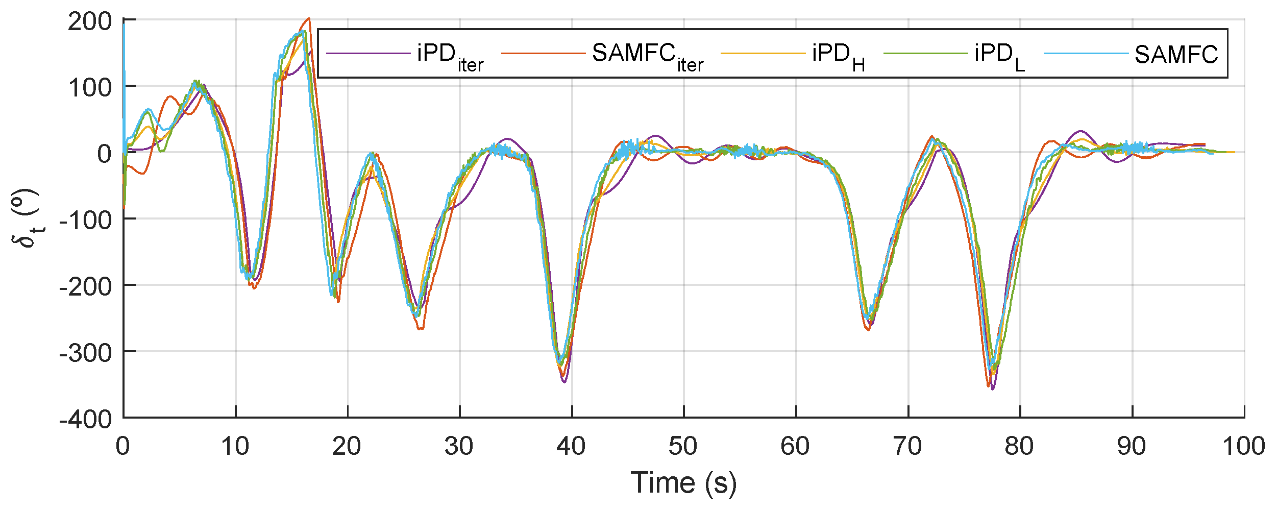
Figure 12 shows the control actions generated by the five controller configurations tested on benchmark trajectory
. It can be seen that controllers with a low
(iPD
and SAMFC) exhibited chattering due to the backlash of the steering actuator. This chattering in the control action did not affect the stability of the feedback system at the longitudinal speeds reached on this trajectory.
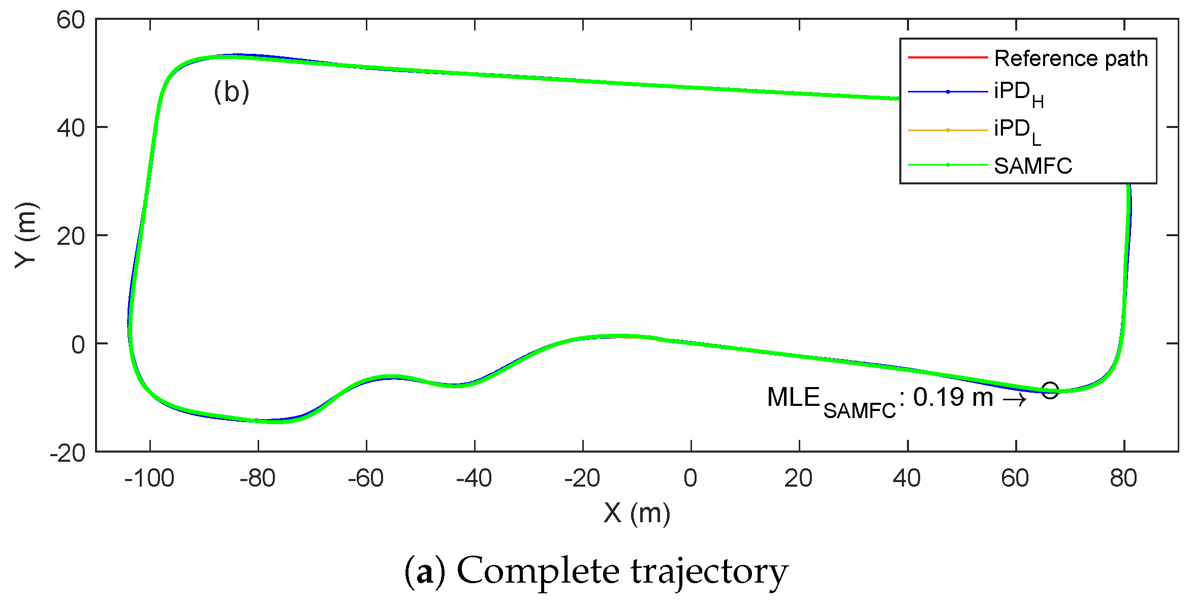
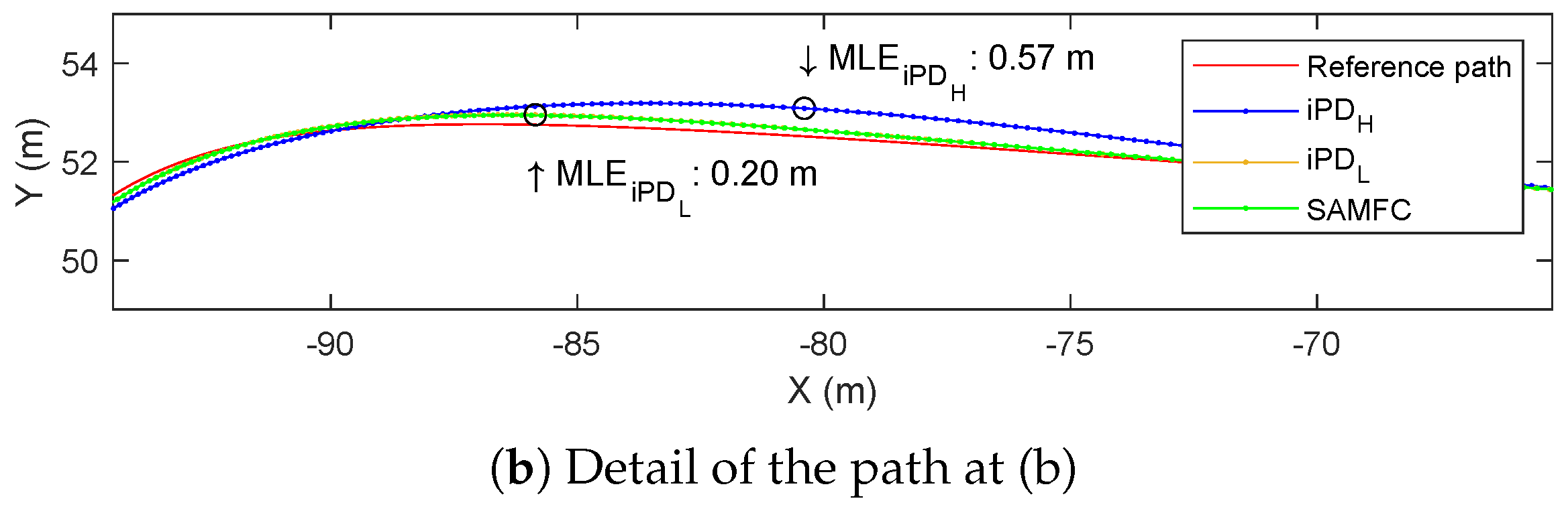
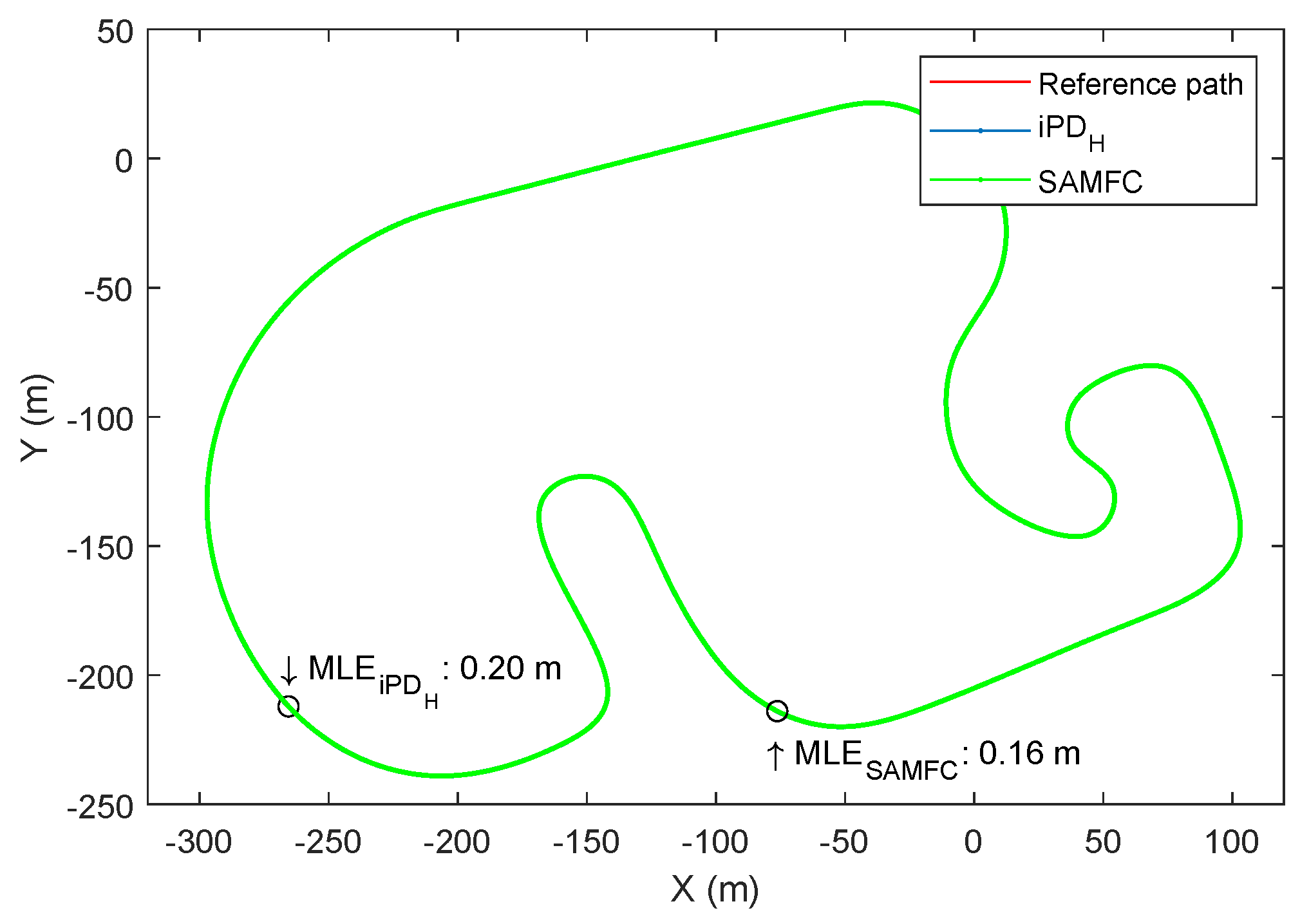
Figure 13 shows the performance of the iteratively designed MFC and SAMFC controllers and
Figure 14 shows the performance of the noniteratively designed MFC and SAMFC controllers tested on benchmark trajectory
. As can be seen, both SAMFC controllers exhibited lower Maximum Lateral Error (MLE) values than the respective original MFC controllers.
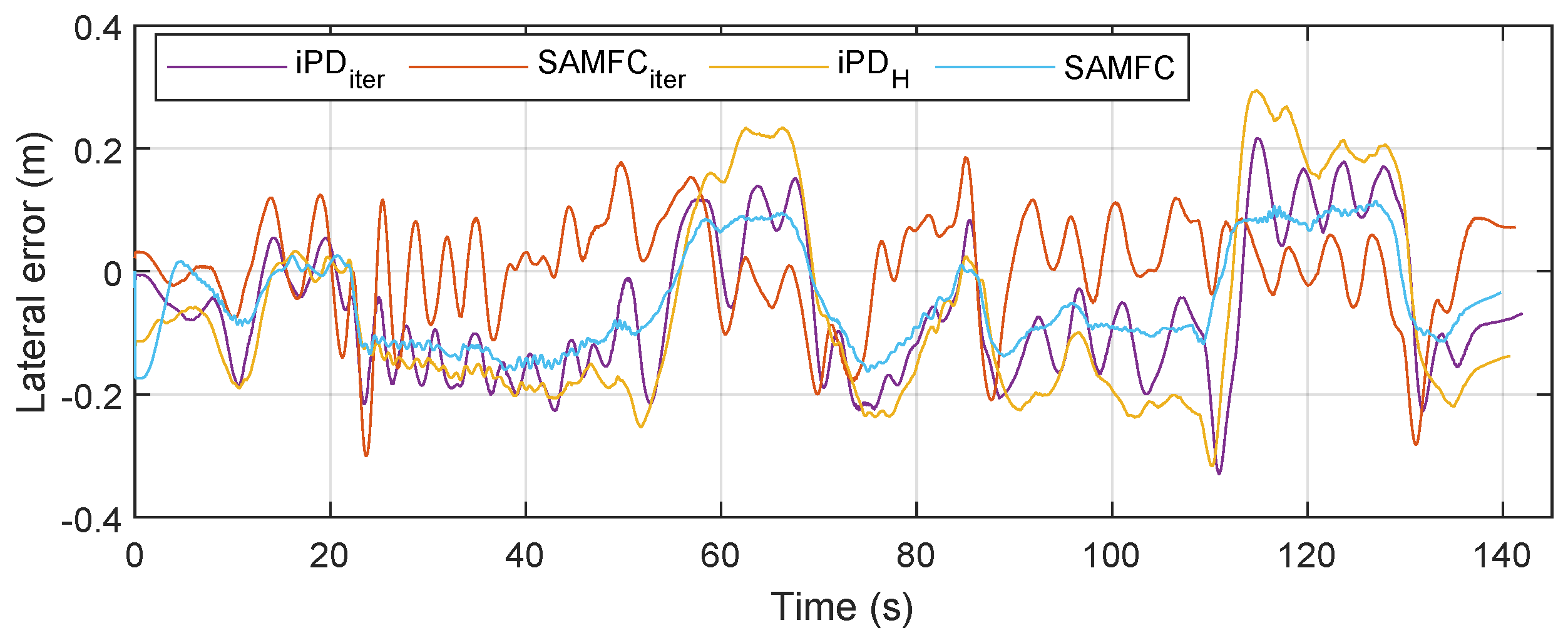
Figure 15 shows the lateral errors of the four evaluated controllers on benchmark trajectory
. It should be noted that iPD
became unstable in the simulation when tested on this trajectory so it was not tested on the experimental platform. As can be seen, the lateral error obtained using the noniteratively designed SAMFC controller was lower than that of the other controllers, which is shown in
Table 7.
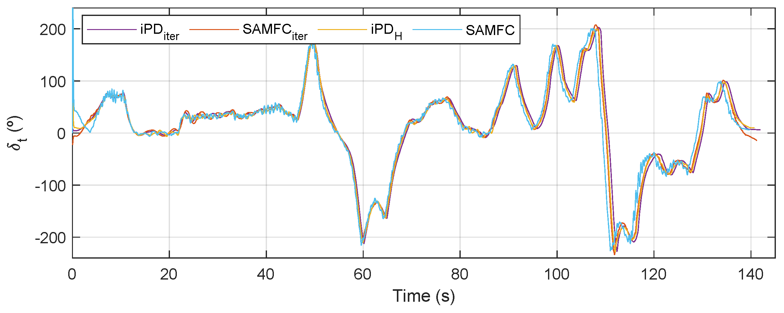
Figure 16 shows the control actions generated by the four controller configurations tested on benchmark trajectory
. It can be seen that all the controllers generated some chattering due to the backlash of the steering actuator. However, it did not affect the stability of the feedback system, as observed on
and reflected in the
values. On the other hand, controllers with a variable
generated a more aggressive response at low speeds than those with a fixed
but they tended to correct the lateral error faster.
Trajectory
had a very different shape, dynamic constraints, and speed profile from
, which was quantitatively reflected in the metrics and the responses of the standard MFC controllers, as shown in
Table 7. On the contrary, the Speed-Adaptive MFC controllers exhibited a more consistent response on both trajectories.
The results presented in this section were obtained on dry asphalt on a sunny day using healthy tires. It should be noted that changing these conditions may affect the reproducibility of the results.


 ,
, 


