
Vehicle Directional Cosine Calculation Method


1
Department of Aerospace Studies, Cornell University, Ithaca, NY 14853, USA
2
Department of Mechanical Engineering (SCPD), Stanford University, Stanford, CA 94305, USA
*
Author to whom correspondence should be addressed.
Vehicles 2023, 5(1), 114-132; https://doi.org/10.3390/vehicles5010008
Submission received: 13 November 2022
/
Revised: 7 January 2023
/
Accepted: 21 January 2023
/
Published: 30 January 2023
(This article belongs to the Special Issue Feature Papers in Vehicles)
Abstract
:Teaching kinematic rotations is a daunting task for even some of the most advanced mathematical minds. However, changing the paradigm can highly simplify envisioning and explaining the three-dimensional rotations. This paradigm change allows a high school student with an understanding of geometry to develop the matrix and explain the rotations at a collegiate level. The proposed method includes the assumption of a point (P) within the initial three-dimensional frame with axes (, , ). The method then utilizes a two-dimensional rotation view (2DRV) to measure how the coordinates of point P translate after a rotation around the initial axis. The equations are used in matrix notation to develop a rotation matrix for follow-on direction cosine matrixes. The method removes the requirement to use Euler’s formula, ultimately, providing a high school student with an elementary and repeatable process to compose and explain kinematic rotations, which are critical to attitude direction control systems commonly found in vehicles.
1. Introduction
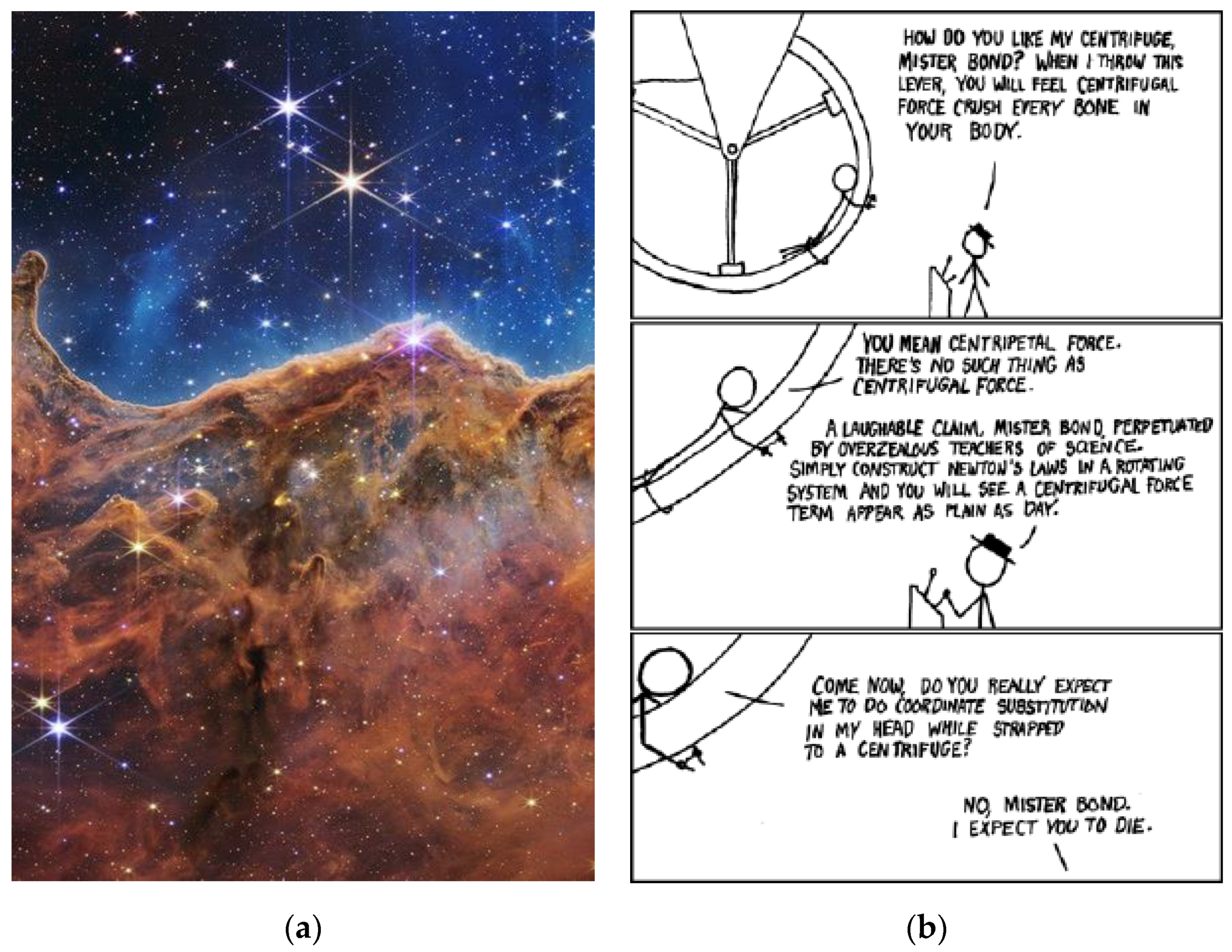
Figure 1.
(a) First images from the James Webb Space Telescope peering into deep space where the “inertial”, non-moving reference frame is often mathematically placed; credits: NASA, ESA, CSA, and STSc [1]. (b) NASA humor over the ubiquity of the difficulty of learning kinematics [2]. Image usage is consistent with NASA policy, “NASA content (images, videos, audio, etc.) are generally not copyrighted and may be used for educational or informational purposes without needing explicit permissions” [3].

When you can measure what you are speaking about and express it in numbers, you know something about it, and when you cannot measure it, when you cannot express it in numbers, your knowledge is of a meagre and unsatisfactory kind. It may be the beginning of knowledge, but you have scarcely in your thought advanced to the stage of a science. Lord Baron Kelvin of Largs [4]
This manuscript describes a step-by-step process to simply develop and understand a set of equations to translate positioning and rotations from one perspective to another. The direction cosine equations are essential to understand the automation of precision motion expressions correctly in attitude direction control systems used in many vehicles. Teaching the concept of an initial axis (, , ) rotating to another axis (, , ) becomes much easier if the initial axis is viewed as a two-dimensional rotation view (2DRV). The new viewpoint of the axis and the rotation makes the mathematics and visual comprehension easier to grasp.
1.1. Educational Importance
Recently, Manurung [5] recommended new methods for teaching kinematics in a journal on education (read by few if any researchers in scientific and mathematical fields). In 2017, Ramma [6] published a public, scathing rebuke of kinematics pedagogy in a popular online blog. The rebuke reported the results of a study of twenty-six physics teachers from twenty-six of a country’s secondary schools who had been teaching for an average of five years to students between 16 and 17 years old. Kinematics typically depicts three-dimensional motion with two-dimensional graphics, while one kinematic representation (the quaternion) involves depicting four-dimensional representations of three-dimensional motion in two-dimensional graphics. The potential for confusion is immediately evident. The Ramma study confirmed the well-known fact that kinematics is challenging to learn, but additionally assessed a key issue laid at the feet of pedagogy and limitations of the topic’s teaching.
Other researchers such as Ayop [7] evaluated the assessments and the resulting kinematics teaching strategies. Shodiqin [8] very recently elaborated on student difficulties in understanding kinematics, while Núñez [9] shortly afterward elaborated on some difficulties themselves, hinting at the relative importance of rethinking the topic’s pedagogical methods. After these recommendations, Moyo [10] performed a focused case study for high schools in Botswana validating the omnipresent sources of difficulties and potential impacts.
To advance the human species’ understanding of the world and the ability to shape future scientists, technicians, and engineers, academics must develop them earlier, faster, and more efficiently. With that in mind, finding and developing more effective ways to deliver academic subject matter to students is critical to future development. Due to the mathematical requirements, rotational kinematics is often a topic that is broached after calculus and linear algebra, if not even later in a student’s academic career. However, with the right tools and perspective, students can be taught the basics of axes rotations at a much earlier stage of educational development.
Laying this foundation at a younger age allows for a more significant expansion of knowledge later. This manuscript’s proposal aims to outline how to efficiently develop this foundational understanding, significantly accelerating students’ academic growth.
1.2. History of Kinematic and Directional Cosine Matrices
The theorems used to translate rigid bodies in Euclidean space date back to 1775 when Euler wrote: “General formulas for the translation of arbitrary rigid bodies” [11]. Over the decades and centuries, the mathematics of the translation of rigid bodies has been refined and expanded, e.g., by Chasles [12] in the early 1800s, by Lord Kelvin in the late 1800s [13], and by Whittaker [14] in the early 1900s.
Several authors [15,16,17,18,19] from the U.S.A.’s National Aeronautics and Space Administration (NASA) and others have published updates. In the late 1960s, Meyer [15] proposed a method for expanding a matrix of direction cosines, while Jordan [16,17] evaluated computation errors using direction cosines and proposed a novel direction cosine algorithm (as proposed in this present manuscript). Kane [18] articulated many challenging aspects of kinematics in the early 1970s. Meanwhile, Haley [19] described manifestations of effects due to the kinematics of integrated robotics. In the 1990s, King [20] illustrated the deleterious effects on the accuracy of global position systems, while Dunn [21] extended the conclusions to include satellite laser ranging. Following the turn of the century, in 2001, Xing [22] proposed alternate forms of attitude kinematics de-emphasizing matrices of nine-direction cosines in favor of three-parameter kinematics (e.g., Euler angles) or four-parameter kinematics (e.g., quaternions, Rodrigues–Gibbs vector, etc.).
Most recently, the significance of direction cosine matrices and their derivation resurged in the 2018 publication by Smeresky [23] which sought to develop more accurate and efficient calculations; and was later revisited by Cole [24] and Sandberg [25] just this year, who tried to discern errors and the resulting deleterious effects in applications. Regardless of which derivation is used, each requires the development of at least two rotational matrices. Ultimately, understanding the development of the direction cosine matrix is critical to understanding kinematics.
1.3. Present-Day Purpose and Innovations Presented
Direction cosine matrices are crucial to attitude direction control systems common in many vehicles such as ships, planes, rockets, satellites, and robotics. While the usual direction construction of cosine matrices equations is still as practical today as when equations were developed, these examples are not immune to adaption or improvement. This work evolves the current method, to provide tools to students to learn, and teachers to instruct three-dimensional kinematic rotations without the without the need to understand Euler’s formula. Simple geometric equations can be used instead of Euler’s formula to develop the rotation matrix to calculate the direction cosine matrices.
Innovations proposed:
1. Two-dimensional rotation view (2DRV) about a third dimension;
2. Development of the rotation matrix equations without Euler’s formula.
Section two describes each rotation matrix’s development where each constructs a direction cosine matrix. Section three outlines how direction cosine matrices work with dynamics, 2DRV, and the proposed process of teaching direction cosine matrix development. Sections four and five provide a conclusion and review other discussion points, respectively.
2. Methods and Results
The approach utilized in this manuscript is based on the rotation of a coordinate system about a fixed point. Any point’s position in the rotated coordinate system can be calculated based on three separate rotations about an axis. Breaking down a single rotation about an axis is equitable to a two-dimensional plane of points rotating about a point. Each rotation can be described and depicted in a 2DRV, as long as the axis and rotation are defined correctly. In a 2DRV, any point in the initial plane can be described in the new plane using the similarity of right triangles and equations of motion functions. The generic rotation conversion equations can be transferred into a matrix format to develop a direction cosine matrix. This method generates the same rotation matrices as the Euler equations but is more straightforward.
2.1. Dynamics
Dynamics is a division of mechanics that deals with how rigid bodies propagate with time in relation to force, mass, momentum, and energy. Dynamics can be dissected into two components: kinetic (linear and rotational forces acting on bodies) and kinematic (motion of bodies regardless of forces). This manuscript only represents a new calculation method of kinematic equations (i.e., direction cosine matrix). However, without understanding some of the basic principles of kinetics, the purpose of the direction cosine matrix can be missed.
The kinetic Equations (1) and (2) describe linear and rotation forces (disturbance and control) on the rigid body. Table 1 outlines all the variables found in Equations (1) and (2). Equations (1) and (2) consider all the linear and nonlinear motion in a fictional non-rotating reference frame utilizing Michel Chasles and Giulio Mozzi’s theorem to combine Newton’s and Euler’s theorems.
The non-rotating reference frame or the inertial frame is a fictional construct that describes a position that is not accelerating or subject to a gravitational field. An inertial frame is developed as no known position in the universe is not accelerating or subject to a gravitational field. As referenced in Figure 1 often deep space is where the fictional inertial frame is placed. If Newton and Euler’s equations of motion were calculated not using an inertial frame of reference, Newtonian laws of motion would not necessarily hold to be true. Once the equations of motion are evaluated in the inertial frame, the equations of motion can be expressed in the body frame and translated into other frames of reference. The kinematics described in section two can translate position and motions into different reference frames [26].
Kinematics is used to translate equations of motion, such as Equations (1) and (2) that are calculated from the inertial frame (later expressed in the body frame) into other reference systems [27]. The non-rotating perspective is required to correctly calculate the disturbance and maneuvering forces, as described in section two for Newtonian and Euler equations. Once the equations of motion are set, translation equations such as direction cosine matrices or quaternions translate the motion into other frames of reference [28]. Quaternions have many beneficial features over classic direction cosine matrices [28]. However, the four-dimensional variables that comprise quaternions are not intuitive to the typical three-dimensional human perspective. Ultimately converting the four-dimension variables to Euler angles makes direction cosine matrix development critical for human–machine interfaces (HMI) such as the ones in vehicles. Understanding the development of the direction cosine matrix is foundational to understanding how the kinematic rotation is calculated.
2.2. Direction Cosine Matrix
Direction cosine matrix equations are based on three separate one-dimensional rotation matrices multiplied in sequence to equate to one three-dimensional rotation equation. It is challenging to present the teaching of three-dimensional rotations, utilizing most teachers’ available two-dimensional resources. Typical examples attempt to show all three dimensions simultaneously and use Euler’s equation to create each rotation matrix, as seen in Figure 2, Figure 3, Figure 4 and Figure 5 and Equations (3)–(7).
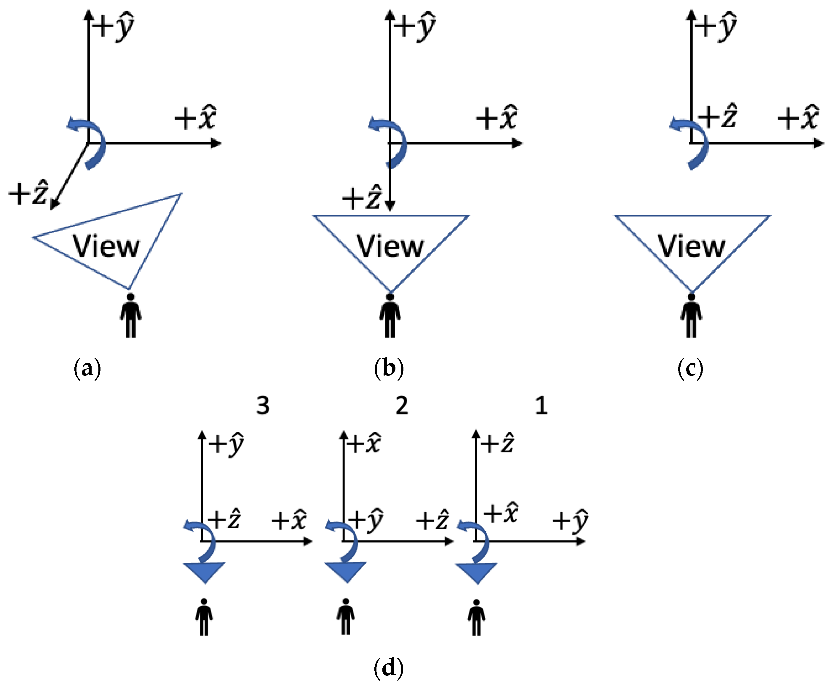
This manuscript uses the 2DRV to help depict and write the translation equations. The 2DRV takes advantage of the fact that a reference frame can be viewed from any aspect. Specifically, 2DRV takes a three-dimensional view and changes the perspective, so only two dimensions are visible. Figure 6a–d depicts the change in perspective. It is important to note that the positive axis being rotated about will face directly out of the page, and the perpendicular positive axes will point up and to the right consistent with a right-hand revolution.
This depiction is helpful because the initial and final axis is colinear, and the only changes happen to points and vectors, not on that axis. Figure 6d depicts what will be referred to as 2DRV for each rotation. The 2DRV simplifies the dimensionality and makes the development of the equations simpler to see and understand. Developing each rotation creates a matrix and must be performed one revolution at a time. Each rotation is identified by the axis it is rotated around. After each matrix is completed, they can be combined to create an overarching direction cosine matrix.
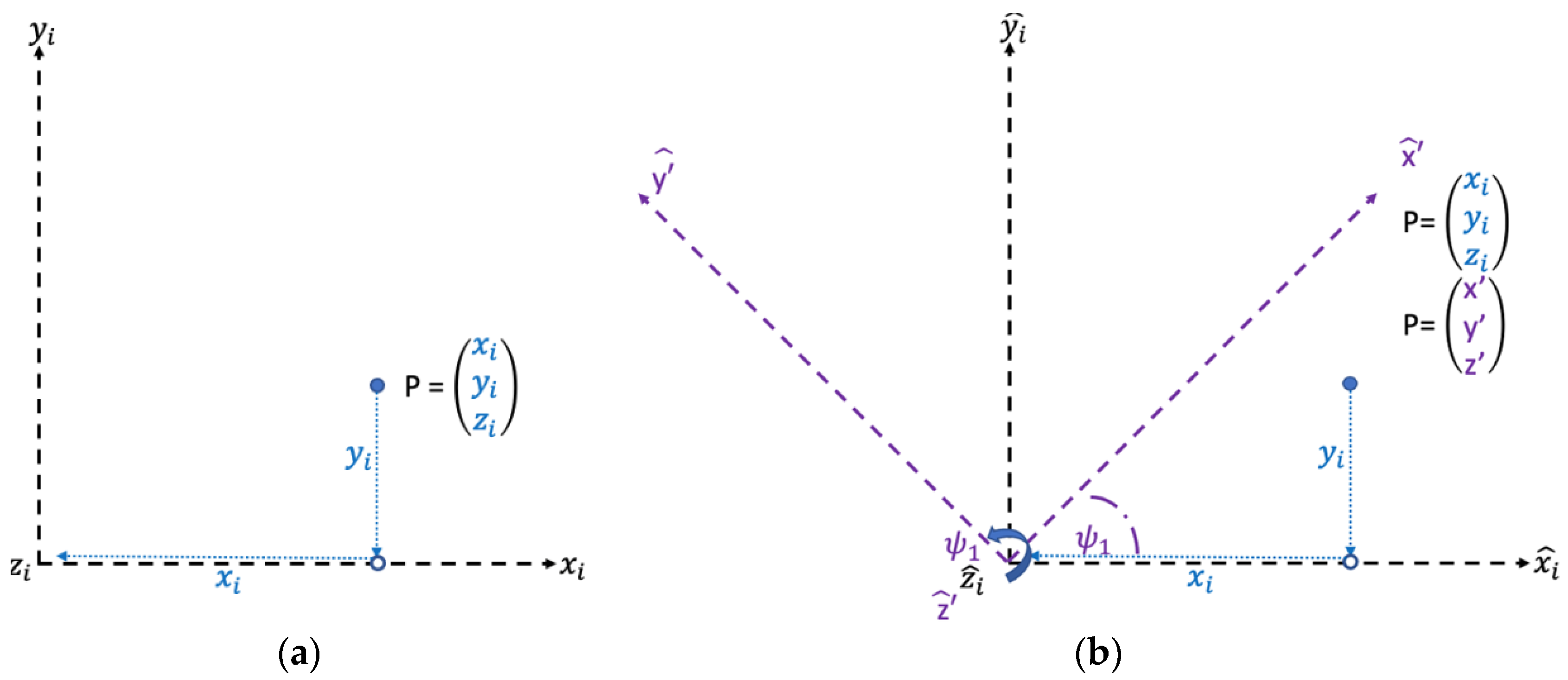
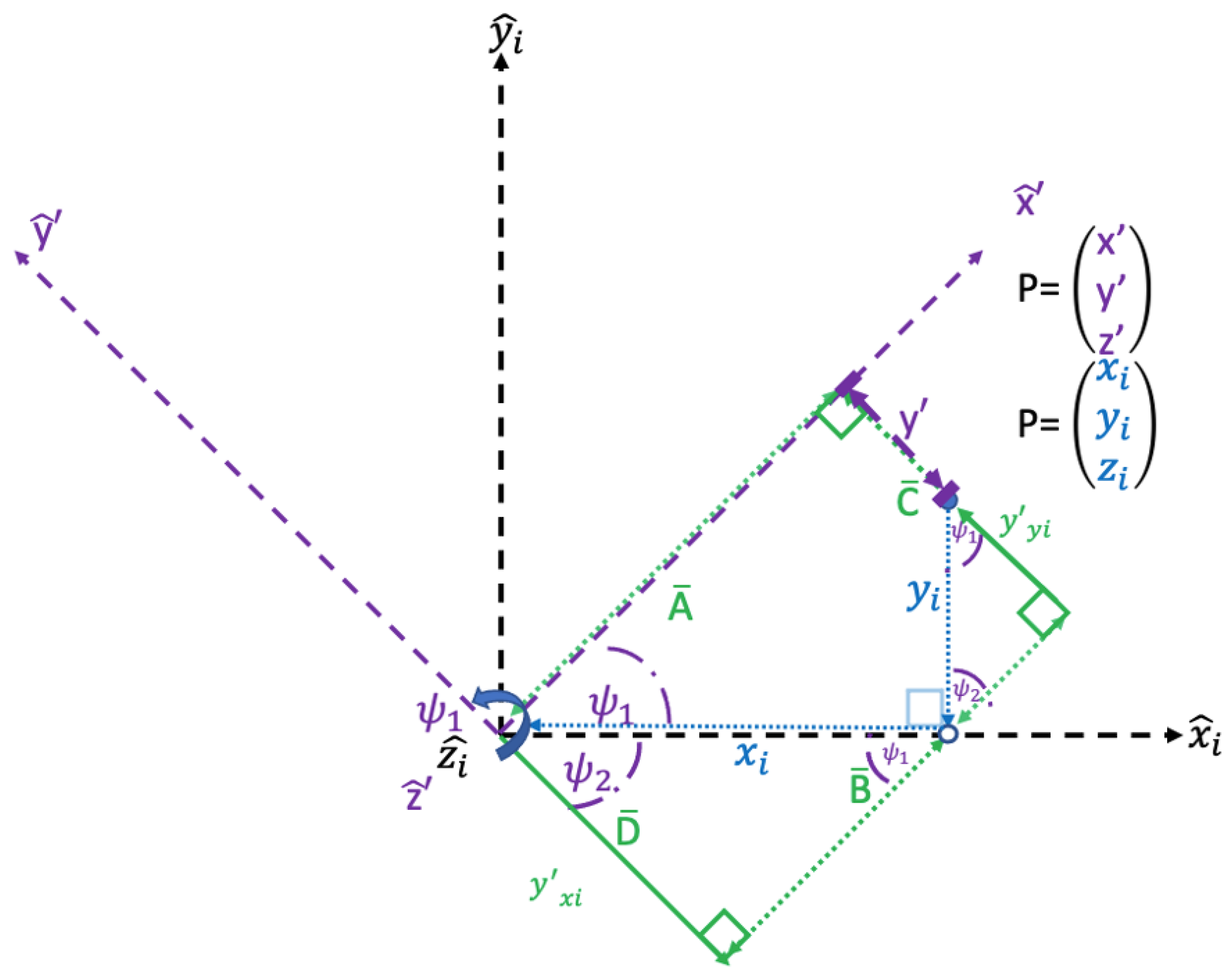
The following direction cosine matrix creation uses the proposed method. Using the 3, 2, and 1 order of rotations, or the 3-, 2-, 1-direction cosine matrix, will take the inertial frame to a body frame. In this description, the order of the rotation also follows the number order. However, it is essential to note that any combination of rotations or translation types can be performed similarly. While the order does not matter, the 3-rotation is the easiest to conceptualize, because a horizontal -axis and a vertical -axis is the most common representation and makes for a solid foundation. First, any point P with coordinates (xi, yi, zi) is placed in the inertial space with axes (, , ), as seen in Figure 7a. Next, a rotation about is rotated by ψ1 to , as seen in Figure 7b. In Figure 7b, point P has different coordinates after the rotation to the new frame of reference. The difference between the coordinates can be calculated using simple equations. Table 2 outlines all the variables found in Figure 7, Figure 8, Figure 9, Figure 10, Figure 11 and Figure 12.
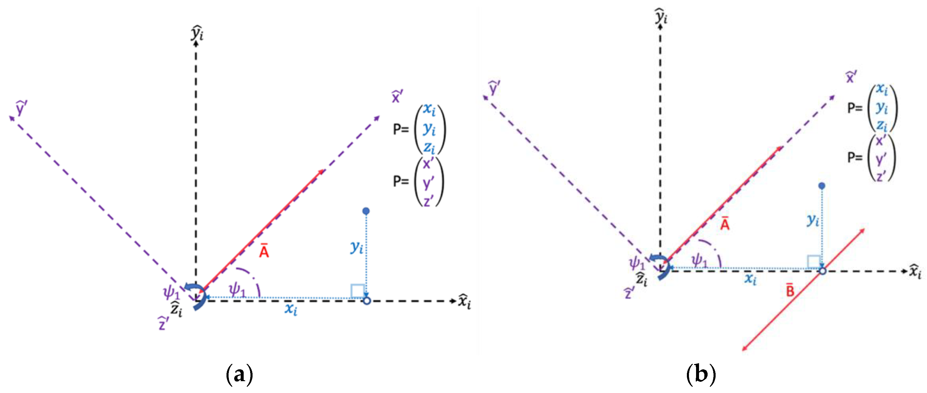
Then, a line can be established along the rotated axis that equates to x′ as seen in Figure 8a, and another similar parallel line with the same length that runs through the (xi,0,0) as seen in Figure 8b.
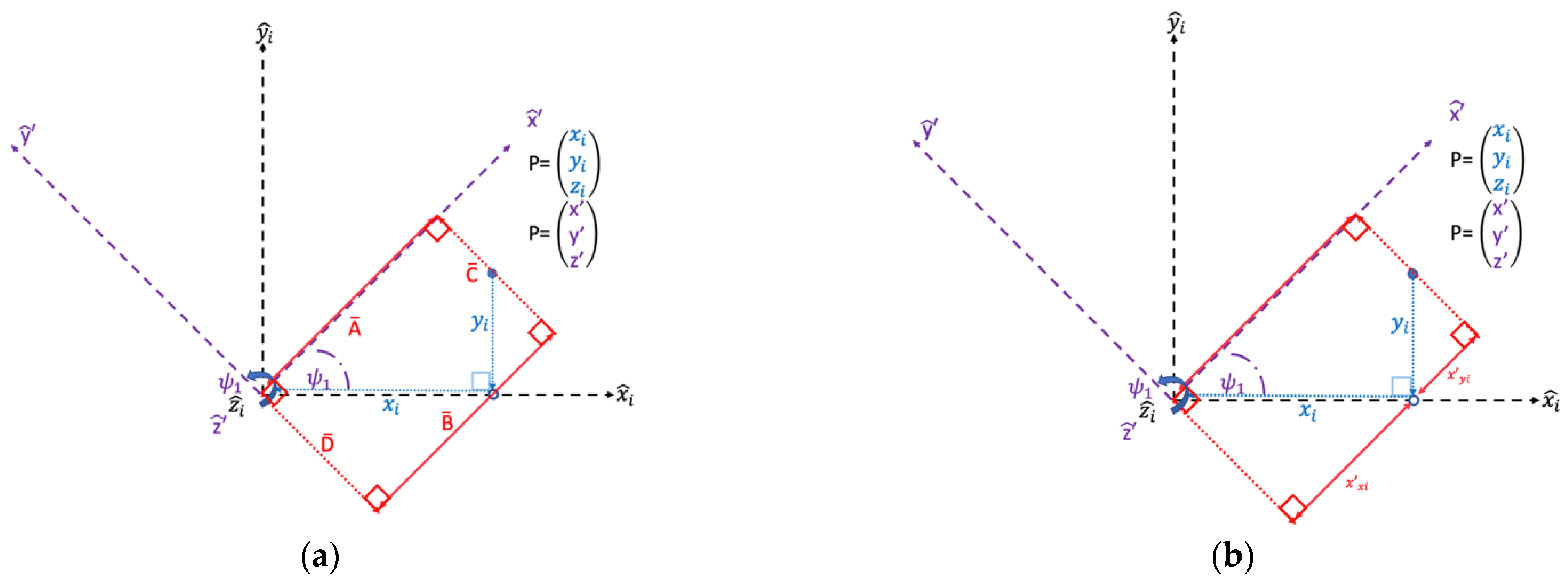
To measure the length of parallel lines , a rectangle can be formed using two other perpendicular similar parallel lines to develop rectangle that starts at the origin, aligns with the new rotation frame, and bisects the point P and (xi,0,0), as seen in Figure 9a. Therefore, lengths of x′ are all equal.
By measuring line in segments, the summation can be used to calculate line . Segments can be identified by which dimension ( or ) of the axis in the initial orientation results in the and as seen in Figure 9b. Therefore, x′ can be calculated by the sum of and , giving Equation (8).
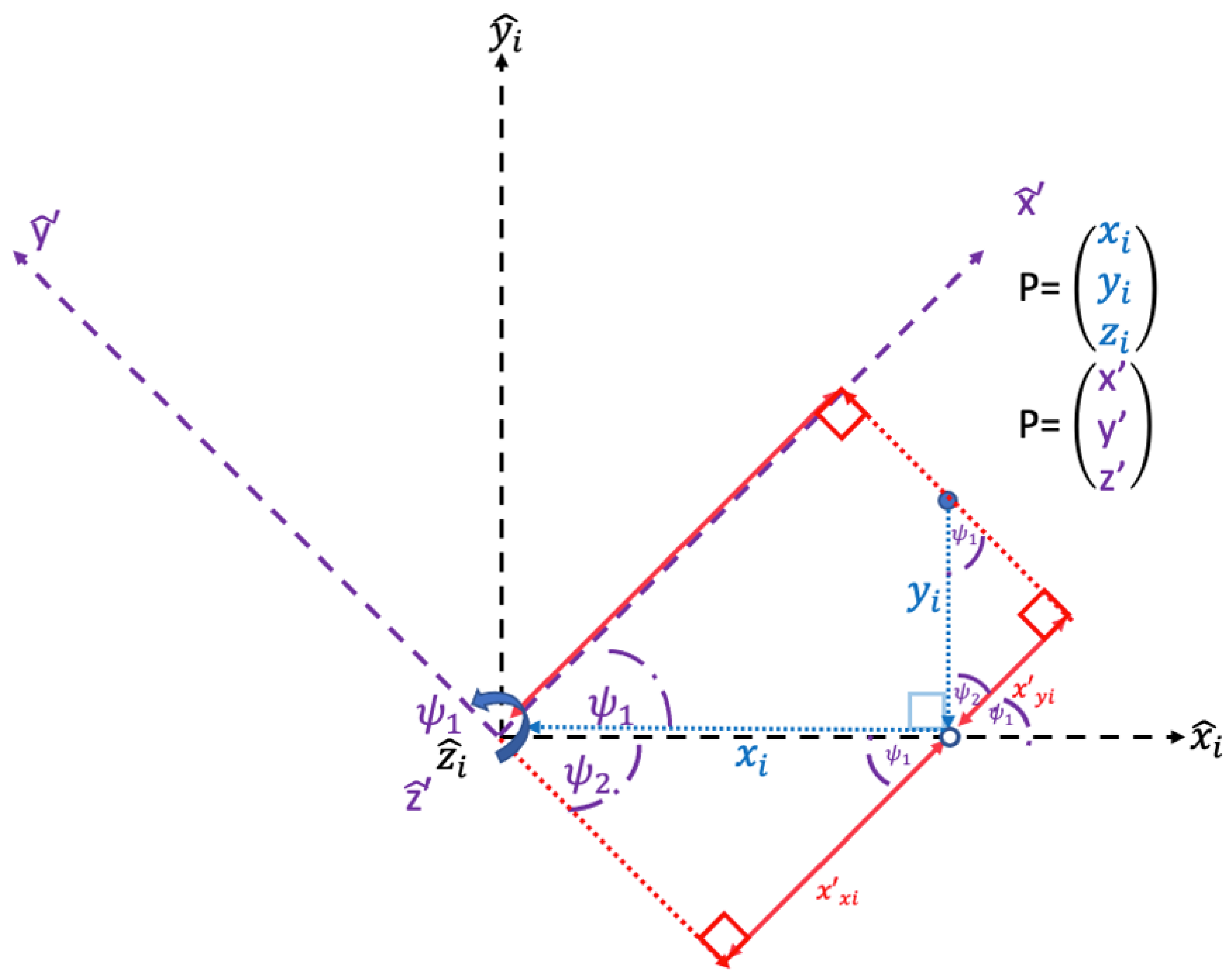
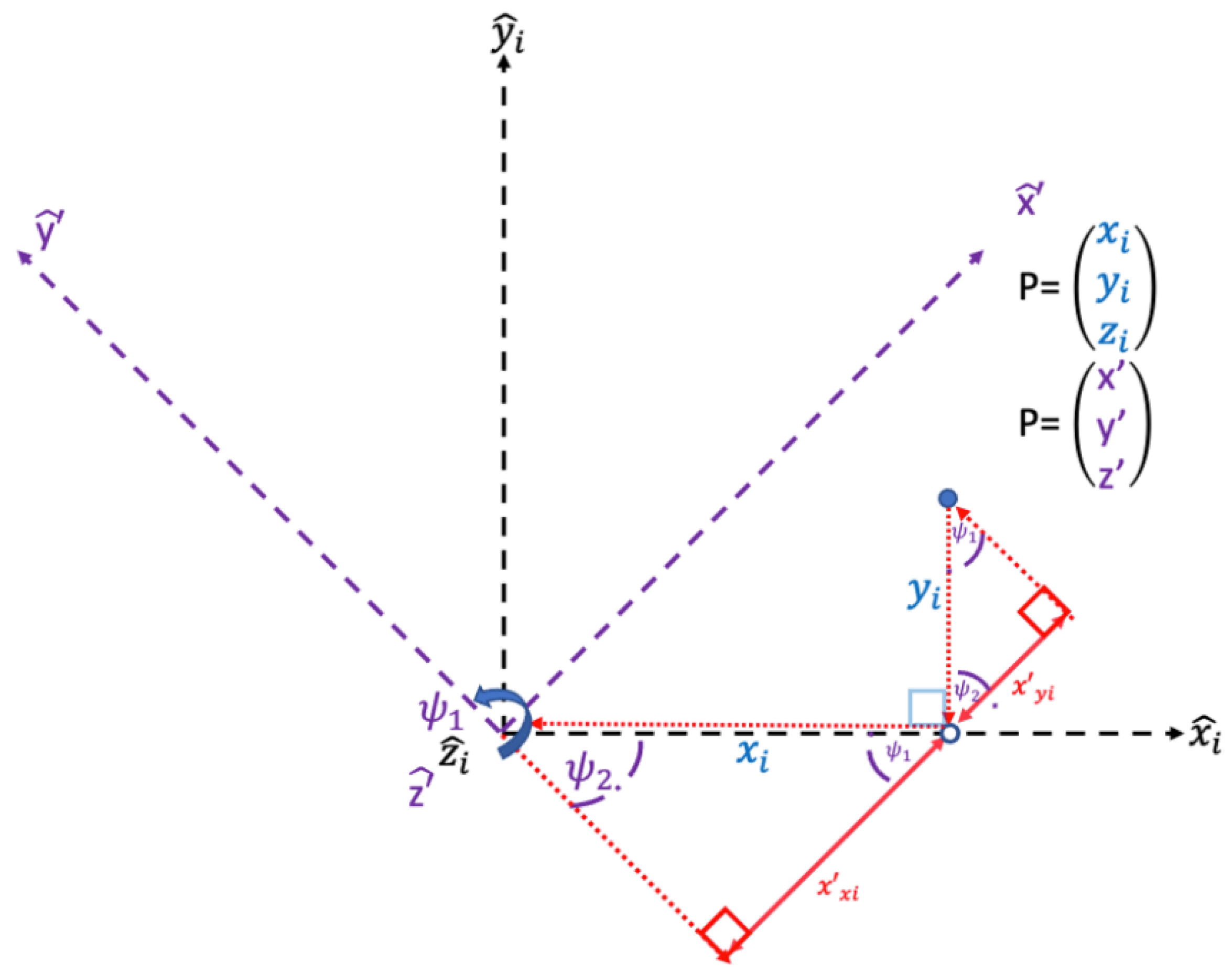
To calculate and , identify is a complementary angle to . One can identify corresponding angles of the transversal of across . Further, an additional complementary angle (formed where and intersect at point P) can be identified as associated with the corresponding angles of where crosses, as seen in Figure 10.
Now two triangles can be identified, as seen in Figure 11, with two defined angles identified as and each with a defined side xi or yi.
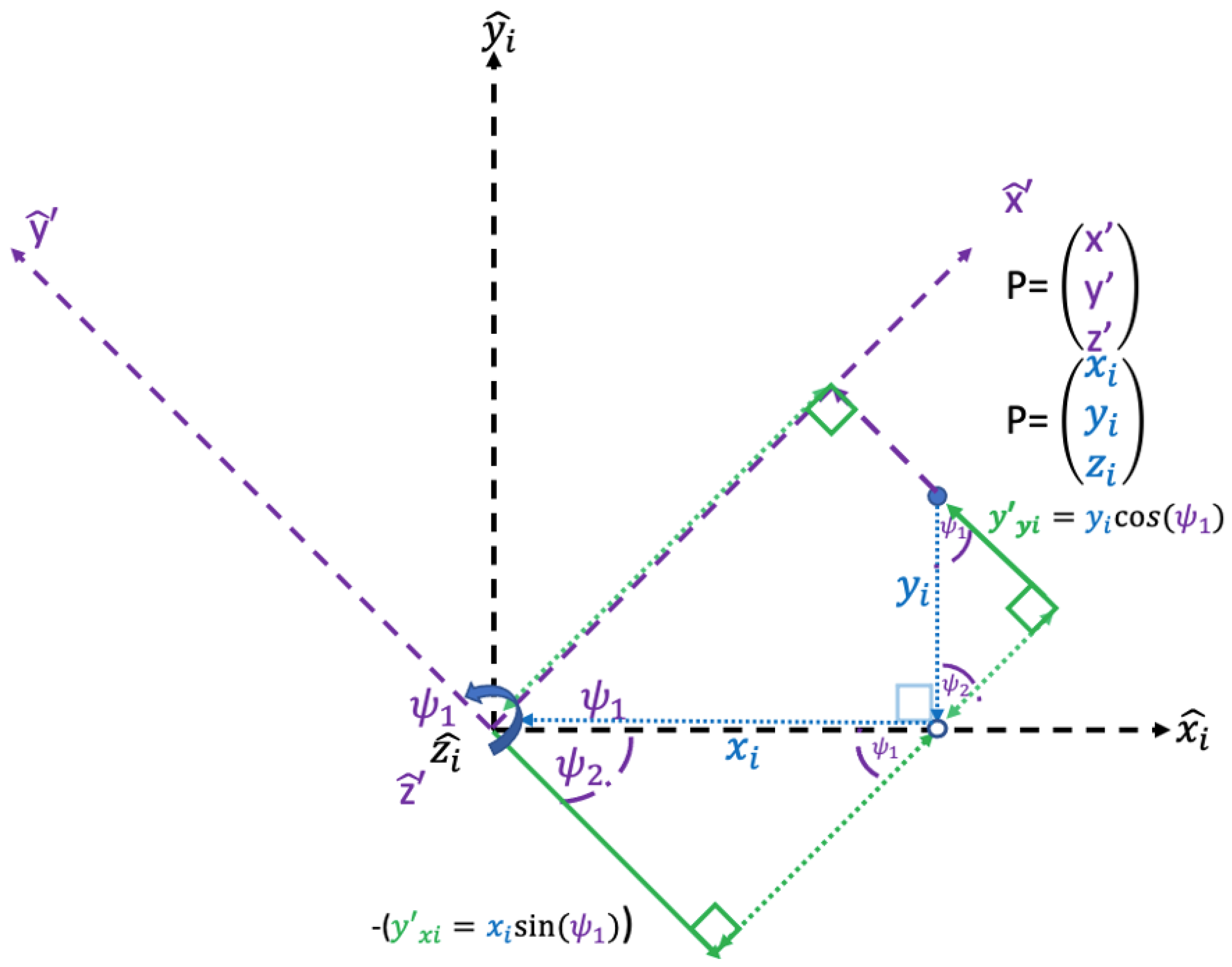
It can be seen that point P’s location on the axis is positive, and because xi and yi are positive, is a summation of each segment and . Therefore, both and are a positive contribution. These conditions define and by and xi or yi in Equations (9) and (10) using the definitions of sine and cosine, as seen in Figure 12. Substituting Equations (9) and (10) into Equation (8) provides Equation (11), the first equation of the 3-rotation matrix.
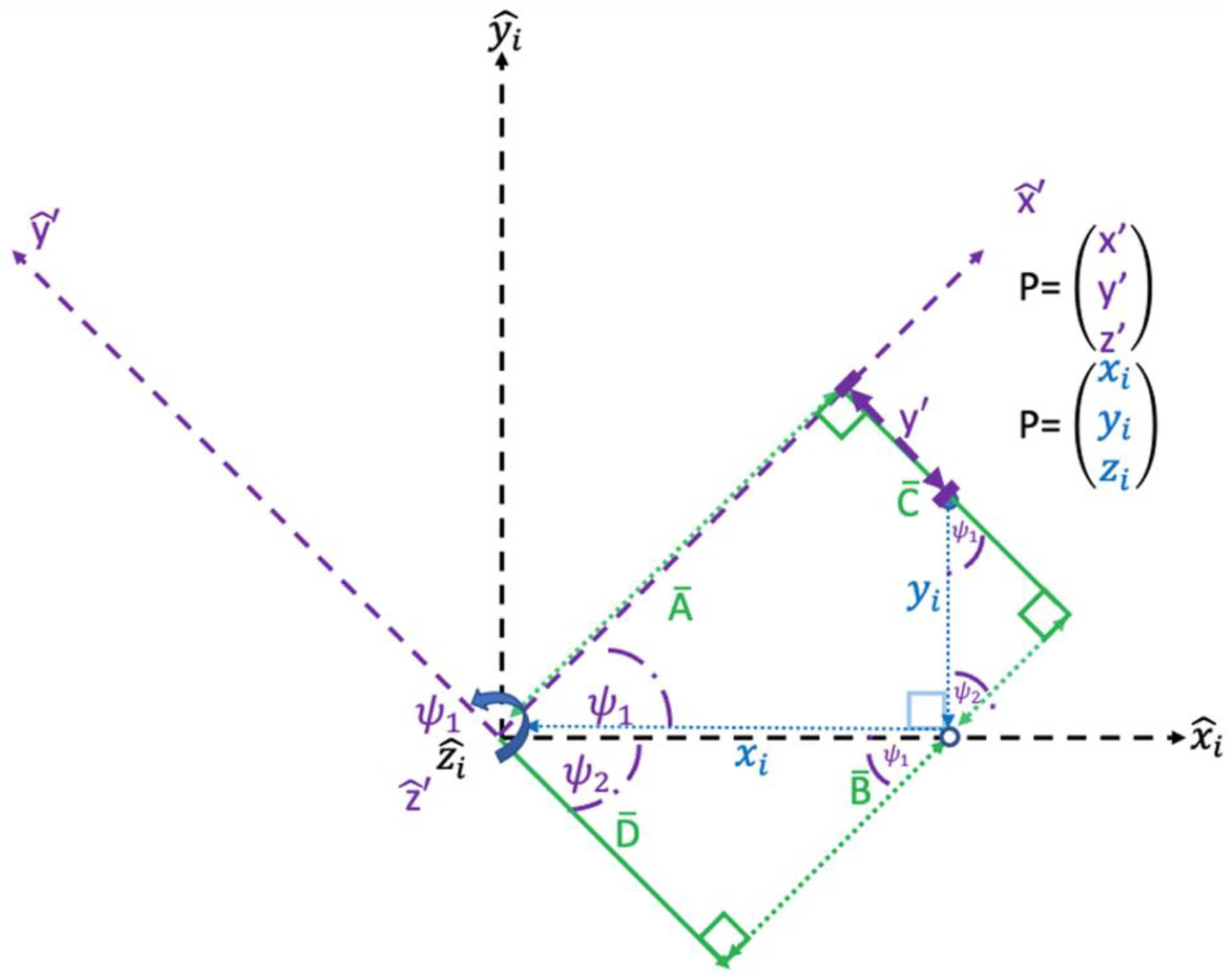
The Equation (12) of the 3-rotation matrix is for y′. To calculate y′ the same rectangle , the two triangles and the defined angles from previous Figure 7, Figure 8, Figure 9, Figure 10, Figure 11 and Figure 12 will be used, except focusing on lines and . Figure 13 shows that P is in the negative axis of y′; and is only a portion of line . As the rotation is about and no additional length is provided to by , so can be multiplied by 0. Table 3 outlines all the variables found in Figure 13, Figure 14 and Figure 15.
By segmenting line into y′ and , one can take the difference of line or and a segment of to calculate y′;. The segments are labeled by the dimension (xi or y) of the initial orientation axis, results in the and as seen in Figure 14. Labeling the pertinent sides of two triangles and in Figure 14, one can use a similar equation to Equation (8) to calculate y′;, and obtain Equation (12).
Term must be the negative difference between and for three reasons: P lies on the negative axis, xi and yi are positive, and because is less than the summation of . Therefore, will be a difference between the segments, and the longer segment must be negative in this case. These conditions define and by and xi or yi in Equations (13) and (14) using the definitions of sine and cosine as seen in Figure 15. Substituting Equations (13) and (14) into Equation (12) provides Equation (15), the second equation of the 3-rotation matrix. As the rotation is about and no additional length is provided to by so can be multiplied by 0.
Equation (16) for is the last equation for this rotation. It is straightforward because the revolution is about to , hence equates to . As the rotation is about to , no additional length is provided to by or so both can be multiplied by 0.
Finally, Equations (11), (15), and (16) can be translated into a matrix format, as seen in Equation (17), the 3-rotation matrix.
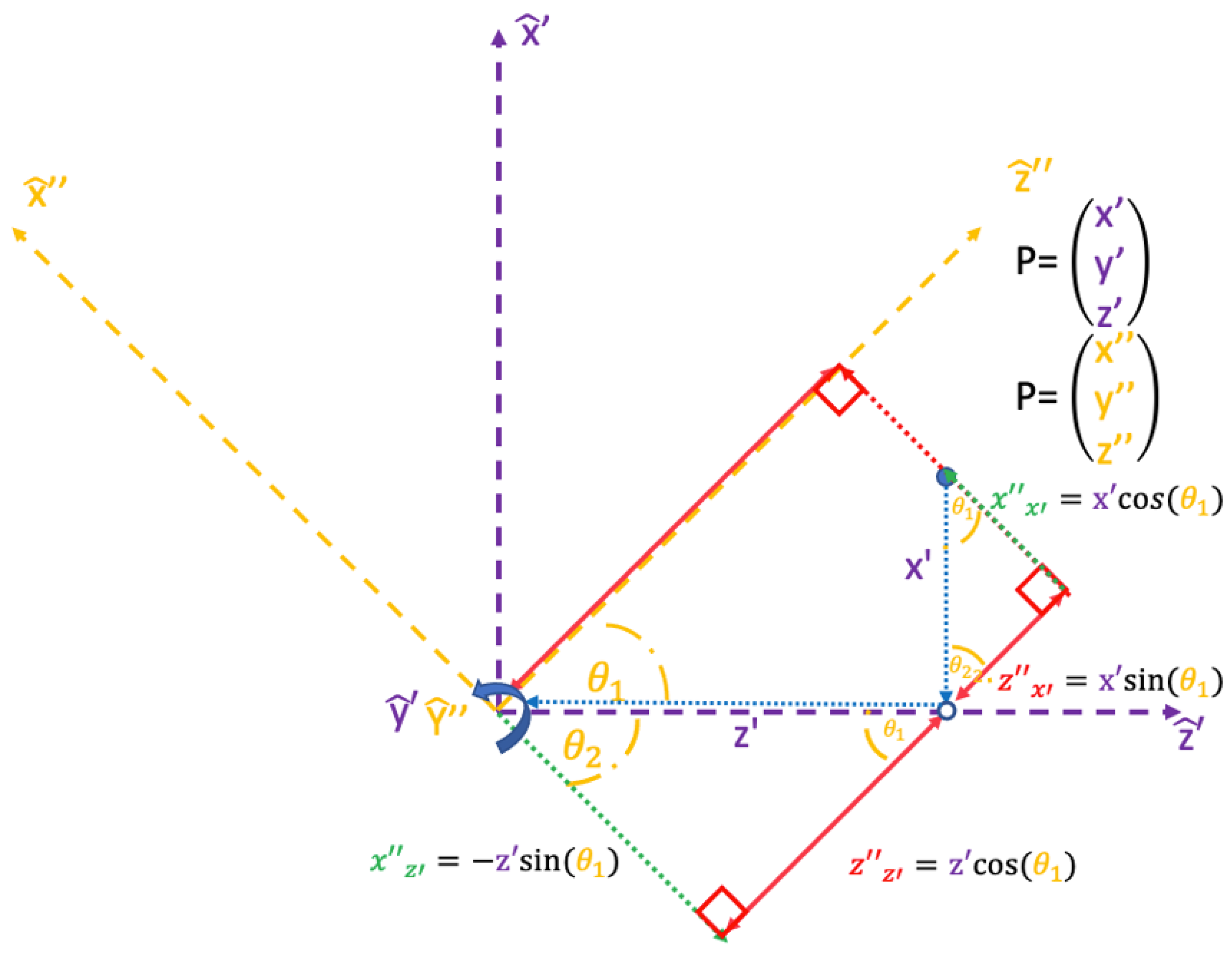
Continuing to the 2-rotation in Figure 16, the axis is rotated by θ1 to . Figure 6d shows the view of the rotation is changed so that the positive axis of the rotating axis ( and ) is viewed as coming directly out of the page. Point P is now taken from (x′;,y′;,z′;) to (x″,y″,z″), similar to Figure 12 and Figure 15. Then, similar equations can be developed using the same mathematics Equations (18)–(27). Table 4 outlines all the variables found in Figure 16.
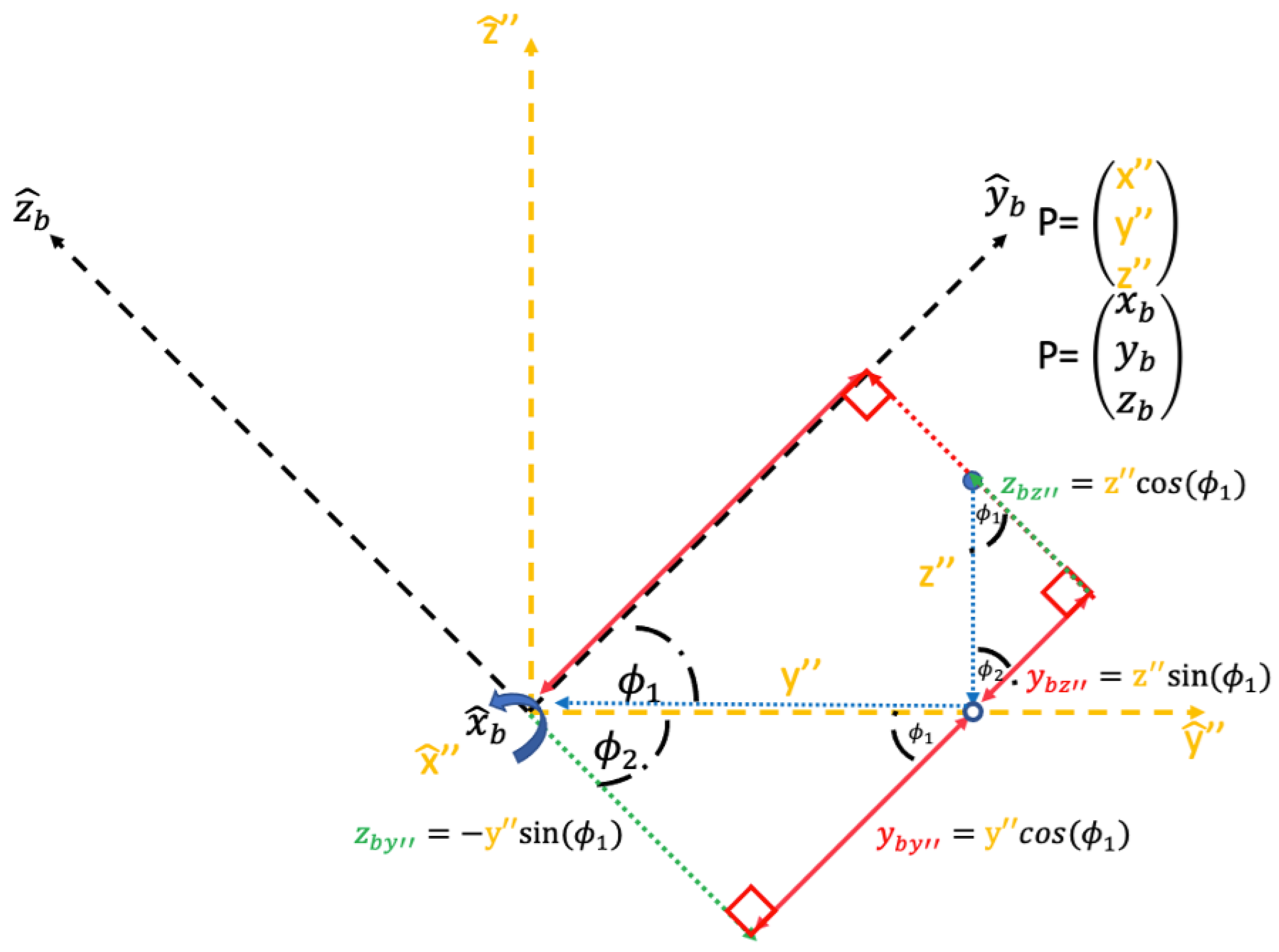
Finally, the 1-rotation in Figure 17 is developed in the same manner as the 3-rotation and 2-rotation. The x″ axis is rotated by to thereby providing the final conversion from (x″, y″, z″) to (,,) coordinates; this provides Equations (28)–(37). Table 5 outlines all the variables found in Figure 17.
Finally, taking each rotation matrix from Equations (17), (27), and (37), the matrices can be multiplied to move from the inertial to the body frame seen in Equation (38). However, the three matrices can be multiplied to develop one overarching direction cosine matrix in a simplified Equation (39), the 3-, 2-, 1-direction cosine matrix.
3. Discussion
The two-dimensional rotation view coupled with the proposed method of creating a direction cosine matrix provides a simplified and repeatable development process. However, there are a couple of recommendations to keep the process simple. Simple decisions on the order of axis rotation, point P’s location, and the rotation angle can present significant difficulty if not adequately thought through.
The 3-rotation is the easiest to conceptualize, since a horizontal -axis and a vertical -axis is the most common representation. This makes the 3-rotation the best to start with, where another rotation may be more challenging to visualize initially. Deciding which axis rotation to start with is not highly consequential to the overall difficulty, but beginning with the 3-rotation may help a new student grasp the concept.
Placing point P at the origin will break the process, so it cannot be recommended. Further it is recommended to use a point P that lies in the positive , , or axis. A negative point P, while not insurmountable, can add unrequired difficulty to the problem. If point P lies in either the negative , , or axis before the rotation, the calculations become more confusing to maintain perspective because it is easy to overlook which variable is negative and how the negative variable affects the equations. Ultimately, if ,, or of point P (,, ) is negative, that negative factor must be maintained through the equations to obtain the proper matrix.
It is recommended to use an acute rotation angle. Using an obtuse rotation angle can further complicate the process; however, similar rectangles, triangles, and their corresponding angles can be found. A remaining question is which angle to utilize for the triangle. The most straightforward method found was to take the cosine and sine of the obtuse angle and find the corresponding acute angles that equate to it, but which may be its opposite sign. When using those equations, the sign of the obtuse angle must be carried throughout the rotation. It is recommended for ease of calculation to start with the 3-rotation, maintain point P in the positive , , and axis, and use an acute angle.
While helpful, using direction cosine matrix for attitude and direction control of vehicles can lead to failure of computations to express specific movements. Specifically, direction cosine matrix fails when kinematic singularities come into play. A kinematic singularity is when the cosine of the rotational angles used for the direction cosine matrix equals zero. It is a regular practice to divide by the cosine of the rotation angle to calculate the Euler-angles rate, so when the cosine of rotation is zero, singularities become an issue. This division by the cosine of the rotation angle when the cosine of the rotation angle is zero causes a calculation error when the systems try to calculate infinity. For these reasons, the quaternions do much of the heavy lifting of the rotations.
4. Conclusions
The method discussed in this paper is very generic and works for all direction cosine matrices. The development of a direction cosine matrix, while a foundational portion of kinematics, is a small part of understanding kinematic engineering. As for most formulae, once the direction cosine matrix is created, the equation does not need to be recreated to be utilized. The process utilization does not negate the importance of the method as it is more about teaching and understanding the process in which a direction cosine matrix operates and is developed.
However, the process could be considered lengthy or confusing compared with other methods. The 2DRV does not allow a member to see all three rotations simultaneously. The 2DRV simplifies a single rotation but does not always help visualize all three rotations. It is recommended that this method be used in tandem with a three-dimensional view to help link the equations to the movement.
Author Contributions
Conceptualization, D.H.; Methodology, D.H.; Software, D.H.; Formal analysis, D.H.; Investigation, D.H.; Data curation, D.H.; Writing—original draft, D.H.; Writing—review & editing, T.S.; Visualization, D.H. and T.S.; Project administration, T.S.; Funding acquisition, T.S. All authors have read and agreed to the published version of the manuscript.
Funding
This research received no external funding. The APC was funded by the corresponding author.
Data Availability Statement
Data may be made available by contacting the corresponding author.
Acknowledgments
Thanks to Garay for teaching me to find my own way of thinking and giving me a high school teacher’s perspective. Kudos to the Jasmine Mally of the Naval Postgraduate School Graduate Writing Center for helping with the grammar and narrative.
Conflicts of Interest
The authors declare no conflict of interest.
References
- NASA. First Images from the James Webb Space Telescope. Available online: https://www.nasa.gov/webbfirstimages (accessed on 30 September 2022).
- NASA. (23a) Frames of Reference: The Centrifugal Force. Available online: https://pwg.gsfc.nasa.gov/stargaze/Sframes3.htm (accessed on 30 September 2022).
- NASA. NASA Image Use Policy. 2022. Available online: https://gpm.nasa.gov/image-use-policy (accessed on 22 May 2022).
- Thomson, W. Popular Lectures and Addresses, Vol. I; MacMillan: London, UK, 1891; p. 80. ISBN 9780598775993. Available online: https://books.google.com/books?id=JcMKAAAAIAAJ&printsec=frontcover&source=gbs_ge_summary_r#v=onepage&q&f=false (accessed on 30 September 2022).
- Manurung, S.; Mihardi, S. Improving the conceptual understanding in kinematics subject matter with hypertext media learning and formal thinking ability. J. Ed. Prac. 2016, 7, 91–98. [Google Scholar]
- Ramma, Y. Physics is Taught Badly Because Teachers Struggle with Basic Concepts. The Conversation: Academic Rigor, Journalistic Flair. Published 29 October 2017. 7.12am EDT. Available online: https://theconversation.com/physics-is-taught-badly-because-teachers-struggle-with-basic-concepts-86083 (accessed on 30 September 2022).
- Ayop, S.; Ismail, M. Students’ understanding in kinematics: Assessments, conceptual difficulties, and teaching strategies. Int. J. Acad. Res. Bus. Soc. Sci. 2019, 9, 1278–1285. [Google Scholar] [CrossRef]
- Shodiqin, M.; Taqwa, M. Identification of student difficulties in understanding kinematics: Focus of study on the topic of acceleration. J. Phys. 2021, 1918, 022016. [Google Scholar] [CrossRef]
- Núñez, R.; Suárez, G.; Castro, A. Difficulties in the interpretation of kinematics graphs in secondary basic education students. J. Phys. 2022, 2159, 012019. [Google Scholar] [CrossRef]
- Moyo, N. Mathematical Difficulties Encountered by Physics Students in Kinematics; Stellenbosch University: Stellenbosch, South Africa, 2020. [Google Scholar]
- Euler, L. Formulae generales pro translatione quacunque corporum rigidorum. Euler Arch. 1776, 20, 189–207. Available online: https://scholarlycommons.pacific.edu/euler-works/478 (accessed on 2 February 2022).
- Chasles, M. Note sur les propriétés générales du système de deux corps semblables entr’eux. Bull. Sci. Math. Astron. Phys. Chem. 1830, 14, 321–326. (In French) [Google Scholar]
- Kelvin, W.; Guthrie-Tait, P. Treatise on Natural Philosophy; Google Play Books; Clarendon Press: Hong Kong, China, 1867; Available online: https://play.google.com/books/reader?id=wwO9X3RPt5kC&pg=GBS.PR8&hl=en (accessed on 30 September 2022).
- Whittaker, E.T. Chapter 1 Kinematical Preliminaries. In A Treatise on the Analytical Dynamics of Particles and Rigid Bodies: With an Introduction to the Problem of Three Bodies; Cambridge University Press: Cambridge, UK, 1917; pp. 4–5. [Google Scholar]
- Meyer, G.; Lee, H.; Wehrend, W. A method for Expanding a Direction Cosine Matrix into an Euler sequence of Rotations. NASA Technical Memorandum X-1384, 1 June 1967. Available online: https://ntrs.nasa.gov/citations/19670017935 (accessed on 30 September 2022).
- Jordan, J. Directional Cosine Computational Error. NASA Technical Report R-304, March 1969. Available online: https://ntrs.nasa.gov/api/citations/19690027619/downloads/19690027619.pdf (accessed on 30 September 2022).
- Jordan, J. An Accurate Strapdown Direction Cosine Algorithm. NASA Technical Report D-5384, September 1969. Available online: https://ntrs.nasa.gov/citations/19690027619 (accessed on 30 September 2022).
- Kane, T.; Likins, P. Kinematics of Rigid Bodies in Spaceflight. NASA Technical Report CR-119361, May 1971. Available online: https://ntrs.nasa.gov/citations/19710021700 (accessed on 30 September 2022).
- Haley, D.; Almand, B.; Thomas, M.; Krauze, L.; Gremban, K.; Sanborn, J.; Kelley, J.; Depovich, T.; Wolfe, W.; Nguyen, T. Evaluation of Automated Decisionmaking Methodologies and Development of an Integrated Robotic System Simulation. NASA Contractor Report 178050, March 1986. Available online: https://ntrs.nasa.gov/citations/19860014816 (accessed on 30 September 2022).
- King, R. Global and Regional Kinematics with GPS. NASA Conference Paper N95-14279, NASA. Goddard Space Flight Center, Satellite Laser Ranging in the 1990s: Report of the 1994 Belmont Workshop, Massachusetts Institute of Technology, Cambridge, MA, USA. 1 November 1994. Available online: https://ntrs.nasa.gov/citations/19950007865 (accessed on 30 September 2022).
- Dunn, P. Global and Regional Kinematics from SLR Stations, NASA Conference Paper N95-14278, NASA. Goddard Space Flight Center, Satellite Laser Ranging in the 1990s: Report of the 1994 Belmont Workshop, Massachusetts Institute of Technology, Cambridge, MA, USA. 1 November 1994. Available online: https://ntrs.nasa.gov/citations/19950007864 (accessed on 30 September 2022).
- Xing, G.; Parvex, S. Alternative Forms of Relative Attitude Kinematics and Dynamics Equations. NASA Goddard Space Flight Center, Greenbelt, Maryland, under Contract NAS5-99163. 1 June 2001. Available online: https://ntrs.nasa.gov/api/citations/20010084965/downloads/20010084965.pdf (accessed on 30 September 2022).
- Smeresky, B.; Rizzo, A.; Sands, T. Kinematics in the information age. Mathematics 2018, 6, 148. [Google Scholar] [CrossRef] [Green Version]
- Cole, D.; Sands, T. Effect of kinematic algorithm selection on the conceptual design of orbitally delivered vehicles. Preprints 2022, 2022020360. [Google Scholar] [CrossRef]
- Sandberg, A.; Sands, T. Autonomous Trajectory Generation Algorithms for Spacecraft Slew Maneuvers. Aerospace 2022, 9, 135. [Google Scholar] [CrossRef]
- Liu, X.; Wang, J. Parallel Kinematics: Type, Kinematics, and Optimal Design; Springer: Cham, Switzerland, 2014. [Google Scholar]
- Dingle, H. On Inertial Reference Frames. Sci. Prog. 1962, 50, 568–583. [Google Scholar]
- Wie, B. Space Vehicle Dynamics and Control; American Institute of Aeronautics and Astronautics: Reston, VA, USA, 1998. [Google Scholar]
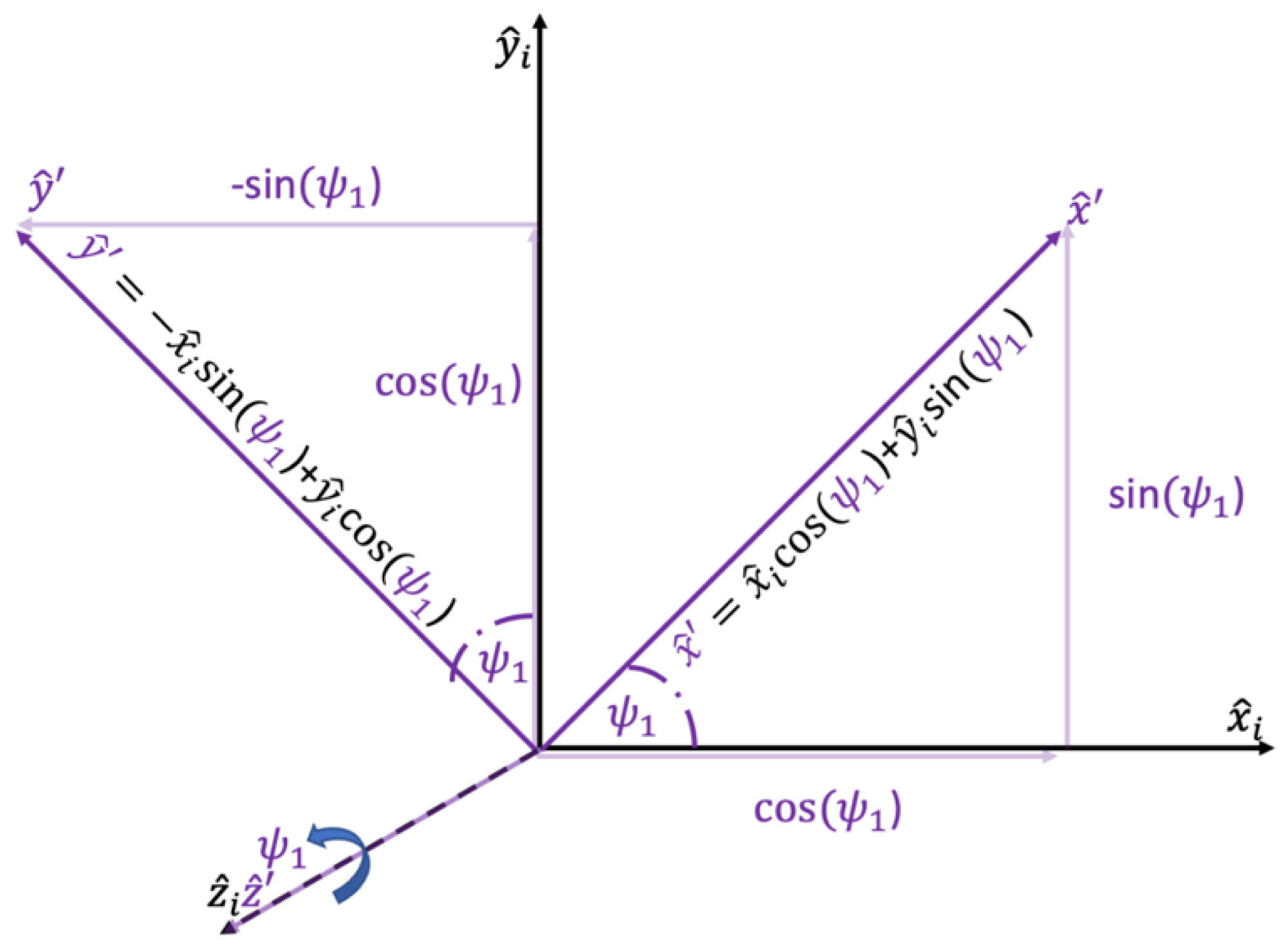
Figure 2.
3-rotation about the and axes [23].
Figure 2.
3-rotation about the and axes [23].

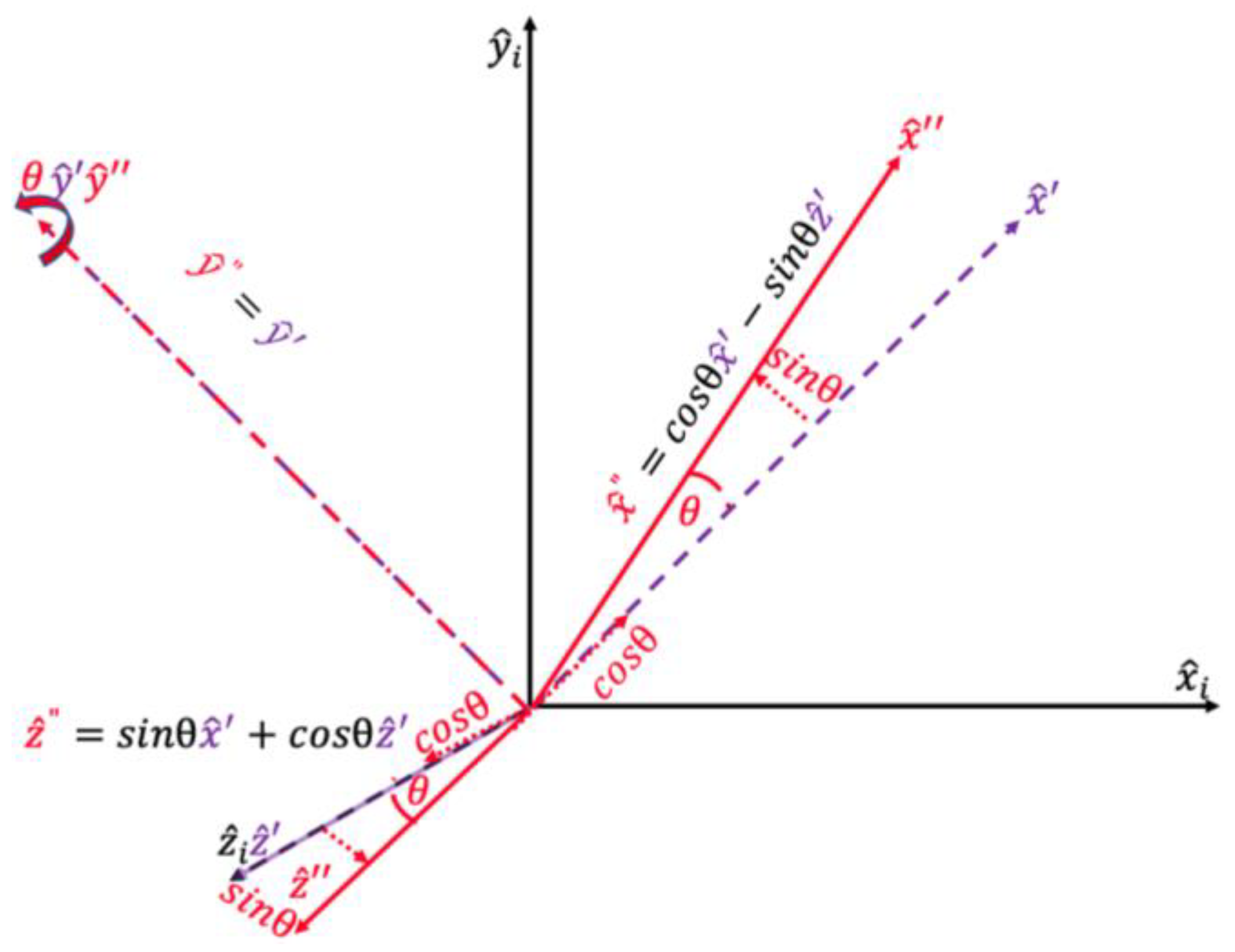
Figure 3.
2-rotation about the and axes [23].
Figure 3.
2-rotation about the and axes [23].

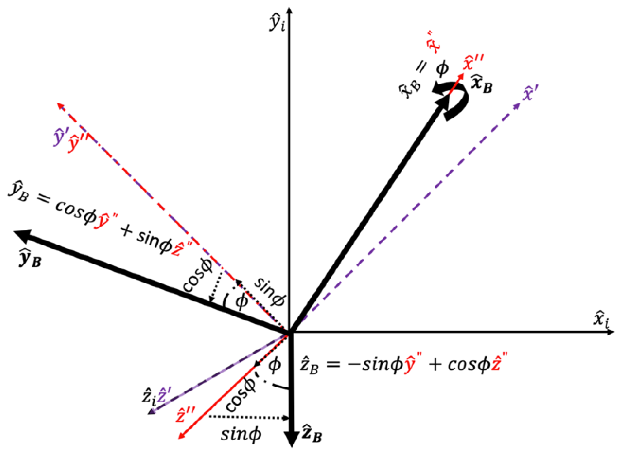
Figure 4.
3-rotation about the and axes [23].
Figure 4.
3-rotation about the and axes [23].

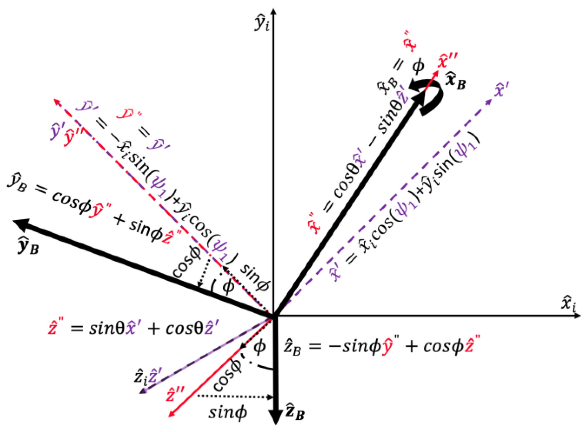
Figure 5.
Compiling the 3-, 2-, 1-rotations in one view with all equations [23].
Figure 5.
Compiling the 3-, 2-, 1-rotations in one view with all equations [23].

Figure 6.
(a–c) Transformation from a three-dimensional view of a rotation to a two-dimensional rotation view (2DRV); (d) the revolutions about the -axis, -axis, or -axis are known as the “3-rotation”, “2-rotation”, and “1-rotation “, respectively.
Figure 6.
(a–c) Transformation from a three-dimensional view of a rotation to a two-dimensional rotation view (2DRV); (d) the revolutions about the -axis, -axis, or -axis are known as the “3-rotation”, “2-rotation”, and “1-rotation “, respectively.

Figure 7.
(a) Point P is dropped within the inertial orientation to develop the direction cosine matrix; (b) 3-rotation about the and axes to develop P’s coordinates in the new reference frame.
Figure 7.
(a) Point P is dropped within the inertial orientation to develop the direction cosine matrix; (b) 3-rotation about the and axes to develop P’s coordinates in the new reference frame.

Figure 8.
(a) 3-rotation about the and axes with the line equivalent to x’; (b) 3-rotation about the and axes with parallel lines equivalent to x’.
Figure 8.
(a) 3-rotation about the and axes with the line equivalent to x’; (b) 3-rotation about the and axes with parallel lines equivalent to x’.

Figure 9.
(a) 3-rotation about the and axes adding parallel lines to create rectangle . (b) 3-rotation about the and axes and dividing into measurable sections and . A determination was made to calculate the equations for x′; first. Both equations of x′; and y′; will be calculated eventually, and the order does not matter— x′; is easier to visualize in this case.

Figure 10.
3-rotation about the and axes, and identifying angles and and pertinent corresponding angles.
Figure 10.
3-rotation about the and axes, and identifying angles and and pertinent corresponding angles.

Figure 11.
3-rotation about the and axes highlighting the pertinent similar right triangles.

Figure 12.
3-rotation about the and axes highlighting segments and equations.

Figure 13.
3-rotation about the and axes using the rectangle , the corresponding angles and , and the same similar triangles built-in Figure 7, Figure 8, Figure 9, Figure 10, Figure 11 and Figure 12, except to measure y′; instead of x′;.

Figure 14.
3-rotation about the and axes highlighting and as part of rectangle .

Figure 15.
3-rotation about the and axes and highlighting equations for segments and .

Figure 16.
2-rotation about the axes to develop P’s coordinates in the new reference frame with all similar angles, shapes, and equations established in Figure 7, Figure 8, Figure 9, Figure 10, Figure 11, Figure 12, Figure 13, Figure 14 and Figure 15.

Figure 17.
1-rotation about the and axes to develop P’s coordinates in the new reference frame with all similar angles, shapes and equations established in Figure 7, Figure 8, Figure 9, Figure 10, Figure 11, Figure 12, Figure 13, Figure 14 and Figure 15.


Table 1.
Proximal variable and nomenclature definitions.
| Term | Definition | Term | Definition | Term | Definition | Term | Definition |
|---|---|---|---|---|---|---|---|
| External resultant force in inertial x-direction | Angular velocity about x-axis | Angular acceleration about x-axis | Moment of inertia along x with respect to x | ||||
| External resultant force in inertial y-direction | Angular velocity about y-axis | Angular acceleration about y-axis | Product of inertia along x with respect to y | ||||
| External resultant force in inertial z-direction | Angular velocity about z-axis | Angular acceleration about z-axis | Product of inertia along x with respect to z | ||||
| Acceleration in inertial x-direction | Velocity in x-direction | External resultant moment | Moment of inertia along y with respect to y | ||||
| Acceleration in inertial y-direction | Velocity in y-direction | Product of inertia along y with respect to z | |||||
| Acceleration in inertial z-direction | Velocity in z-direction | Moment of inertia along z with respect to z |
Table 2.
Proximal variable and nomenclature definitions for Figure 7, Figure 8, Figure 9, Figure 10, Figure 11 and Figure 12.
| Term | Definition | Term | Definition | Term | Definition | Term | Definition |
|---|---|---|---|---|---|---|---|
| x-axis in the inertial non-rotating reference frame | xi | Point P’s location on x-axis in the inertial non-rotating reference frame | x-axis in the new rotated reference frame about the axis to the axis | Point P’s location on the -axis after the rotation about the axis to the axis | |||
| y-axis in the inertial non-rotating reference frame | yi | Point P’s location on y-axis in the inertial non-rotating reference frame | y-axis in the new rotated reference frame about the axis to the axis | Point P’s location on the -axis after the rotation about the axis to the axis | |||
| z-axis in the inertial non-rotating reference frame | zi | Point P’s location on z-axis in the inertial non-rotating reference frame | z-axis in the new rotated reference frame about the axis to the axis | Point P’s location on the -axis after the rotation about the axis to the axis | |||
| Line B segment determined by angle ψ1 and the hypotenuse xi | . | Line B segment determined by the angle ψ1 and hypotenuse yi | ψ1 | Angle of rotation about the axis to the axis | ψ2 | Complementary angle to ψ1 | |
| Line equivalent to Point P’s measurement along the axis | Line parallel and equidistant to crossing through (xi,0,0) | Line perpendicular to and equidistant to crossing through point P | Line perpendicular to and equidistant to crossing through the origin/rotation point | ||||
| Rectangle developed by lines ,, |
| Term | Definition | Term | Definition | Term | Definition | Term | Definition |
|---|---|---|---|---|---|---|---|
| x-axis in the inertial non-rotating reference frame | xi | Point P’s location on x-axis in the inertial non-rotating reference frame | x-axis in the new rotated reference frame about the axis to the axis | Point P’s location on the -axis after the rotation about the axis to the axis | |||
| y-axis in the inertial non-rotating reference frame | yi | Point P’s location on y-axis in the inertial non-rotating reference frame | y-axis in the new rotated reference frame about the axis to the axis | Point P’s location on the -axis after the rotation about the axis to the axis | |||
| z-axis in the inertial non-rotating reference frame | zi | Point P’s location on z-axis in the inertial non-rotating reference frame | z-axis in the new rotated reference frame about the axis to the axis | Point P’s location on the -axis after the rotation about the axis to the axis | |||
| Line segment determined by angle ψ1 and the hypotenuse xi | . | Line segment determined by the angle ψ1 and hypotenuse yi | ψ1 | Angle of rotation about the axis to the axis | ψ2 | Complementary angle to ψ1 | |
| Line equivalent to point P’s measurement along the axis | Line parallel and equidistant to crossing through (xi,0,0) | Line perpendicular to and equidistant to crossing through point P | Line perpendicular to and equidistant to crossing through the origin/rotation point | ||||
| rectangle developed by lines ,, |
Table 4.
Proximal variable and nomenclature definitions for Figure 16.
Table 4.
Proximal variable and nomenclature definitions for Figure 16.
| Term | Definition | Term | Definition | Term | Definition | Term | Definition |
|---|---|---|---|---|---|---|---|
| x-axis in the new rotated reference frame about the axis to the axis | Point P’s location on the -axis after the rotation about the axis to the axis | x-axis in the rotated reference frame about the axis to the axis | Point P’s location on the, x’’-axis after the rotation about the y’. axis to the axis | ||||
| y-axis in the new rotated reference frame about the axis to the axis | Point P’s location on the -axis after the rotation about the axis to the axis | y-axis in the rotated reference frame about the axis to the axis | Point P’s location on the y’’.-axis after the rotation about the y’. axis to the axis | ||||
| z-axis in the new rotated reference frame about the axis to the axis | Point P’s location on the -axis after the rotation about the axis to the axis | z-axis in the rotated reference frame about the axis to the axis | Point P’s location on the z’’.-axis after the rotation about the y’. axis to the axis | ||||
| Determined using the same techniques as | . | Determined using the same techniques as . | θ1 | Angle of rotation about the axis to the axis | θ2 | Complementary angle to θ1 | |
| Determined using the same techniques as | . | Determined using the same techniques as . |
Table 5.
Proximal variable and nomenclature definitions for Figure 17.
Table 5.
Proximal variable and nomenclature definitions for Figure 17.
| Term | Definition | Term | Definition | Term | Definition | Term | Definition |
| x-axis in the rotated reference frame about the axis to the axis | Point P’s location on the, x’’.-axis after the rotation about the, y’. axis to the axis | x-axis in the rotated reference frame about the axis to the axis | Point P’s location on the, x-b..-axis after the rotation about the, y’’. axis to the axis | ||||
| y-axis in the rotated reference frame about the axis to the axis | Point P’s location on the, y’’.-axis after the rotation about the, y’. axis to the axis | y-axis in the rotated reference frame about the axis to the axis | Point P’s location on the, y-b..-axis after the rotation about the, y’’. axis to the axis | ||||
| z-axis in the rotated reference frame about the axis to the axis | Point P’s location on the, z’’.-axis after the rotation about the, y’. axis to the axis | z-axis in the rotated reference frame about the axis to the axis | Point P’s location on the, z-b..-axis after the rotation about the, y’’. axis to the axis | ||||
| Determined using the same techniques as | . | Determined using the same techniques as . | Angle of rotation about the axis to the axis | Complementary angle to | |||
| Determined using the same techniques as | . | Determined using the same techniques as . |
Disclaimer/Publisher’s Note: The statements, opinions and data contained in all publications are solely those of the individual author(s) and contributor(s) and not of MDPI and/or the editor(s). MDPI and/or the editor(s) disclaim responsibility for any injury to people or property resulting from any ideas, methods, instructions or products referred to in the content. |
© 2023 by the authors. Licensee MDPI, Basel, Switzerland. This article is an open access article distributed under the terms and conditions of the Creative Commons Attribution (CC BY) license (https://creativecommons.org/licenses/by/4.0/).
Share and Cite
MDPI and ACS Style
Hall, D.; Sands, T. Vehicle Directional Cosine Calculation Method. Vehicles 2023, 5, 114-132. https://doi.org/10.3390/vehicles5010008
AMA Style
Hall D, Sands T. Vehicle Directional Cosine Calculation Method. Vehicles. 2023; 5(1):114-132. https://doi.org/10.3390/vehicles5010008
Chicago/Turabian StyleHall, Derek, and Timothy Sands. 2023. "Vehicle Directional Cosine Calculation Method" Vehicles 5, no. 1: 114-132. https://doi.org/10.3390/vehicles5010008