

Predictive Optimal Control of Mild Hybrid Trucks

1
Mechanical Engineering Department, Purdue University, West Lafayette, IN 47907, USA
2
Mechanical Engineering Department, Indiana University Purdue University, Indianapolis, IN 46202, USA
*
Author to whom correspondence should be addressed.
Vehicles 2022, 4(4), 1344-1364; https://doi.org/10.3390/vehicles4040071
Submission received: 11 October 2022
/
Revised: 9 November 2022
/
Accepted: 25 November 2022
/
Published: 1 December 2022
(This article belongs to the Topic Vehicle Dynamics and Control)
Abstract
:Fuel consumption, subsequent emissions and safe operation of class 8 vehicles are of prime importance in recent days. It is imperative that a vehicle operates in its true optimal operating region, given a variety of constraints such as road grade, load, gear shifts, battery state of charge (for hybrid vehicles), etc. In this paper, a research study is conducted to evaluate the fuel economy and subsequent emission benefits when applying predictive control to a mild hybrid line-haul truck. The problem is solved using a combination of dynamic programming with backtracking and model predictive control. The specific fuel-saving features that are studied in this work are dynamic cruise control, gear shifts, vehicle coasting and torque management. These features are evaluated predictively as compared to a reactive behavior. The predictive behavior of these features is a function of road grade. The result and analysis show significant improvement in fuel savings along with NOx benefits. Out of the control features, dynamic cruise (predictive) control and dynamic coasting showed the most benefits, while predictive gear shifts and torque management (by power splitting between battery and engine) for this architecture did not show fuel benefits but provided other benefits in terms of powertrain efficiency.
1. Introduction
Due to the rapid explosion of automobile technology in the trucking line-haul segment, there has been a tremendous need for making the trucking sector more fuel efficient, safe, and clean. Consequently, researchers from all over the globe are focusing on a better fuel optimal powertrain operation by leveraging a wide variety of control and system architecture. Platooning, predictive control, hybrid systems, externally-heated emission devices are a few such principal areas of research. There is a lot of work conducted in this space and the global optimal problem can be set up in a variety of ways, with different constraints and objectives. While most of the research focused on a single objective for the optimal solution, a more robust and holistic solution is proposed in this paper. Several robust multi-objective non-linear optimal control strategies are analyzed and based on the current requirements and tradeoffs; dynamic programming is selected to solve the global optimal problem. The following literature highlights the current state of technology as it relates to optimization methodologies for heavy-duty line-haul trucks. Xiaodong et al. discussed an interesting adaptive energy management strategy based on an equivalent consumption minimization strategy (ECMS) by using real-time traffic information described by the average speed, average acceleration, and standard deviation of speed for different road sections [1]. Guo et al. (2022) proposed a novel dual-adaptive equivalent consumption minimization strategy (DA-ECMS) for the complex multi-energy system in a four-wheel drive parallel hybrid electric vehicle (PHEV) [2]. The paper proposed multi-energy system optimizations by introducing categories of future driving conditions to adjust the equivalent factors. A self-organizing neural network and grey wolf optimizer (GWO) was adopted to classify the driving condition categories and optimize the multi-dimensional equivalent factors offline. Zecchi et al. designed a new fuel cell mathematical model for a hybrid powertrain [3]. The innovation of this model lies in the versatility and modularity of the model, which is open to modifications and features a low computational burden, making it suitable for testing new solutions by performing first design and sizing calculations. Another paper [4] assesses the impact of an eco-driving training program on fuel savings and reduction of CO2 emissions in a well-designed field trial. This methodology includes different types of road sections under various traffic conditions and a systematic method to evaluate specific impacts of eco-driving. A simple optimization method for a battery electric vehicle (BEV) is designed by Scalaretta et al. [5]. Direct, indirect methods for solving optimal problems using spectral collocation, shooting methods, etc., are discussed in [6,7,8]. The paper [9] presents a simulation study of various battery electric vehicle (BEV) types to compare their performance when driving on real-road drive cycles to highly optimized eco-driving cycles. The results of the simulation confirmed that eco-driving has a high potential to reduce energy consumption for all types of BEVs. This study also compares the impact of eco-driving on conventional vehicles to comparable BEVs. The authors in [10] implemented strategies to minimize fuel consumption by limiting instantaneous vehicle specific power while maintaining average speed and conserving total distance. The paper [11] explains how a truck driver controls his vehicle with the motive of maintaining a desired velocity while keeping the fuel consumption as low as possible. This is achieved by estimating oncoming operation points of the powertrain and optimal choice of inputs. This information is used as an input in an algorithm for the implementation of a predictive gearshift program and predictive cruise controller. In the paper [12], a novel predictive technology is used to incorporate the cruise set speed along with a gear shift point. The numerical-based algorithm used a combination of nonlinear dynamics constraint and objective cost. The mixed integer problem due to the gear choice is solved partially by the outer convexification process. Benefits are shown on real-world and artificial routes. The paper [13] explores how information about future road slopes can be used in a heavy truck with an aim of reducing fuel consumption without increasing total travel time. The longitudinal behavior of the vehicle is controlled by determining throttle and brake levels and which gear to engage. In the paper [14], a novel predictive control scheme is used for energy management in hybrid trucks driving autonomously on the highway. This scheme uses information from a GPS together with speed limits along the planned route to schedule charging and discharging of the battery, the vehicle speed, the gear and the decision of when to turn off the engine and drive electrically. The paper [15] presents an optimal strategy for heavy-duty trucks that minimizes fuel consumption in urban areas. This strategy uses an online convex model predictive control strategy that balances a trade-off between reducing braking effort and tracking optimal velocity. The paper [16] introduces a model predictive control algorithm which attempts to reduce the cost of operation of heavy trucks with cruise control application based on road topology information obtained through GPS positioning and 3D maps. The paper [16] proposes implementation of predictive optimal algorithms operating the truck at economically favorable operation points by considering the costs of operation and dynamics of the vehicle. This approach considers GPS positioning and 3D maps for slope, curve and speed limit information of future road segments. The paper [17] proposes a model predictive control method to control the clutch engagement process and effectively shorten the torque interruption, thus enhancing the gear downshift quality. The paper [18] explains a way of exploiting vehicular on-board prediction for a limited time horizon and minimizing the auxiliary energy consumption of the electric cooling system through real-time optimization. The paper [19] provides a comparison of three strategies using model predictive control with the objective of minimizing fuel consumption for a heavy-duty truck. The three strategies are: a time-based formulation that penalizes braking effort in place of fuel consumption, a simplified approach to the first strategy, and a distance-based convex formulation that maintains a tradeoff between energy expenditure and tracking of the coarsely optimized velocity. In the operation of line-haul trucks, fuel costs have a large impact on total cost of ownership. The paper [20] attempts to solve the problem of obtaining a trade-off between minimizing the fuel consumption and simultaneously maximizing the vehicle speed, thus eventually decreasing time-related fixed costs. The paper [21] explores learning-based predictive cruise control and the impact of this technology on increasing fuel efficiency for commercial trucks by implementing a predictive cruise control model which uses future road conditions and solves for cost-effective course of action. The paper [22] provides a comparison of three strategies using model predictive control with the objective of minimizing fuel consumption for a heavy-duty truck. Two of these three strategies can then be adapted to accommodate the presence of traffic and optimally navigate signalized intersections using infrastructure-to-vehicular communication. The paper [23] illustrates how optimizing the power split among different energy sources in electric trucks should be performed to ensure safety, drag reduction and energy consumption. The paper [24] investigates the fuel-saving potential of predictive optimal control methods for the engine cooling system in conventional trucks. The advantages of this approach are the recovery of brake energy and the balance of energy sources to minimize total energy. The paper [25] attempts to reduce ECMS’s calculation load by proposing an adaptive simplified ECMS-based strategy for a parallel plug-in hybrid electric vehicle. The paper [26] proposes a novel real-time energy management strategy for parallel hybrid electric vehicles. This approach uses adaptive ECMS which sets the time-varying equivalent factor. Hybrid electric vehicles have been known to be a feasible option to reduce fuel consumption and emissions. The paper [27] proposes an adaptive energy management system consisting of off-line and online parts to improve the energy efficiency of a parallel hybrid electric bus. The offline part focuses on the precision of a driver’s driving style based on the hybrid algorithm. The online part incorporates the driver’s driving style into equivalent consumption minimization strategy.
There are numerous attempts made at solving a holistic fuel-efficient problem for different applications, but none has been proposed for a mild-hybrid class 8 truck using look ahead corridor information. In this work, the attempt was to find the global predictive fuel and emissions efficient behavior in terms of predictive control of cruise speed, gear shift, engine ON/OFF coasting and intelligent SOC management for a mild hybrid driven class 8 truck. The problem is also solved using a cost minimization based on battery internal temperature of the battery pack. None of the literature above solved a true global optimal problem for multiple correlated controls with multiple interacting states for a mild hybrid architecture using predictive look-ahead knowledge of the road grade. A holistic optimal solution is proposed in this paper along with analysis on realizable vs. non-realizable benefits for each control lever.
2. One-Dimensional Longitudinal Vehicle Dynamics
A reduced order one-dimensional longitudinal forward torque model is used in this work. A model order reduction is necessary to solve the optimal problem since each additional order of the model will increase a system state and will affect the solver. A class 8 heavy duty truck, with a 48 V mild hybrid system configured to run in a parallel power assist mode, is used in this paper. The electric machine is connected to the driveshaft via a single gear/clutch assembly at the transmission output shaft. It is also very important to explore emissions reduction while studying the key control features since emissions standards are growing more stringent. Subsections below will briefly discuss the sizing for different components in such a configuration. The platform architecture is not very important here and, in fact, the proposed algorithm and methods are applicable to any platform, even to a conventional powertrain. A few hypotheses and assumption about the powertrain architecture are:
- Benefits of the predictive algorithm proposed are relative to baseline. Hence, a particular powertrain architecture will not affect the proposal in this work
- Axle and tire models are not explicitly defined except for using a rear axle ratio and coefficient of rolling resistance
- The battery management system is a simple SOC tracking (between 25% and 75%) with a look-up-based model for open-circuit voltage and internal resistance [28].
- Charging and discharging cycle is based on driver demand power. The hybrid system is charged within limits based on battery internal temperature limits whenever the driver demand power is negative. This is the case for regenerative braking. If the SOC is more than 75%, the hybrid system is not charged any more, even if the driver demand power is negative.
The below subsections will briefly describe the sizing and type of the key components of the power train used in this work. As a side note, it is not mandatory to select the same powertrain to realize the benefits of the algorithm proposed in this work. The proposal in this work can be applied to any powertrain by selectively framing the problem based on the states/controls of the system.
2.1. Internal Combustion Engine
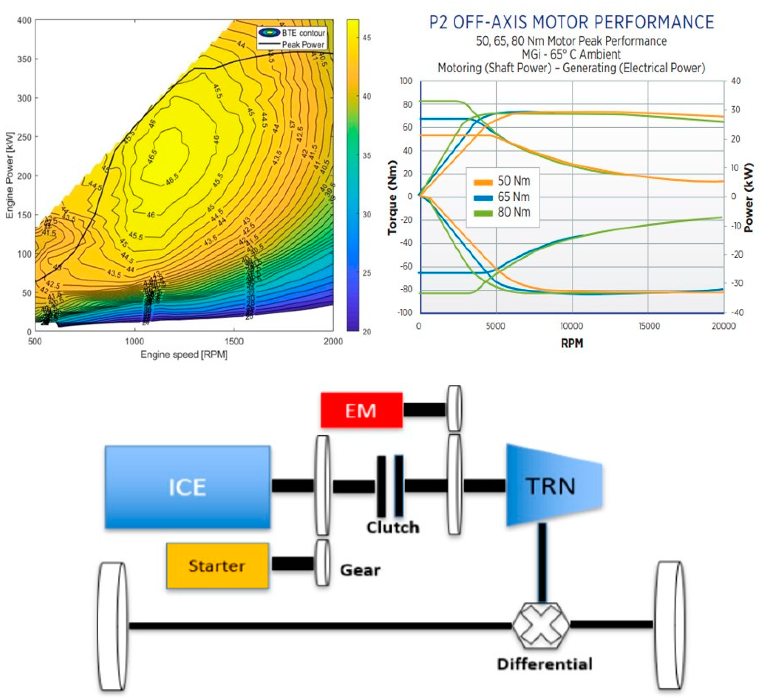
The engine is from the 15L diesel family which has a power rating of 298–373 kW and a torque rating of 1966–2508 N.m. The fuel map is made up manually to mimic an engine efficiency 47%, as shown in Figure 1. It is a 6-cylinder inline configured system [29] with a single maximum brake thermal efficiency (BTE) contour.
2.2. Electrification System
The electrification system in this configuration consists of a motor generator and an energy storage device. Since the chosen configuration is a mild 48 V hybrid system, the motor of choice is a BorgWarner P2 Off Axis motor, which supports a torque range up to 80 Nm. Top right plot in Figure 1 shows the torque and power characteristics of the chosen motor as a function of its rated speed in RPM. It is worth noting that beyond 4000 RPM, the torque starts decreasing and power is flattened. The continuous power of the electric machine is 15 kW with peak torque raging between 50–80 Nm. There are several choices for a 48 V energy storage system. In this work, a simple configuration from A123 Systems is selected [28]. The battery is moderately sized with 8 Ah capacity and a nominal operating temperature of 25 °C. At these settings it can provide continuous power of 15 kW. A simple thermal model for the battery is designed to model the heat loss by the battery [31]. An active cooling system is also in place to increase the rate of heat loss by the battery [32]. The map-based values for the OCV and internal resistance are calculated and tuned based on these models in simulation. Since the battery is small and limited by power, proper heat management of the battery is necessary to utilize its full range of power capability.
The SOC is estimated using coulomb counting method [33,34,35] which is a very efficient and simple way to calculate SOC.
The SOC state is divided by the vehicle speed. This is to reformulate all vehicle dynamics in the distance domain. This change from time domain is necessary to solve the problem for an independent time solution. This fact will be discussed further in the problem formulation section.
2.3. Transmission System
The transmission system is a 12-speed overdrive system from Eaton [36]. There are 12 forward ratios and 2 reverse ratios. Only the top 4 gear ratios are used since the velocity profile used is taken from the highway drive cycle. The gear ratios are documented in Table 1 and are referred from Eaton© [36]. The top 4 gear ratios used are [0.776, 1, 1.3, 1.7] It can support a maximum gross vehicle weight (GVW) of 49,895 kg and supports a maximum torque of 2508 N.m. The shift points for the transmission are made up using vehicle speed reference. The way it is derived as a function of vehicle speed and operator throttle so that at cruising speed the transmission stays at top gear. It is also carried out in a way to keep the engine speed within the best operable BTE region.
2.4. Drive Line and Chassis
The chassis is from a typical line-haul application. A gross vehicle weight (GVW) of 49,895 kg is used in this study, which fits nicely into the component requirements as well as a standard load-carrying measure. The number of wheels in this configuration are 18. A rear axle ratio of 2.64 is used, which gives a lot of low-end torque propagation at startup and does not let the engine operating point go too high at top gear. The optimization result is strongly coupled to these chosen components. Specifically, the chassis components are key players in deciding the vehicle dynamics and optimal fuel numbers since they impact the vehicle speed directly. Table 2 shows the base vehicle parameters which are used in the simulation.
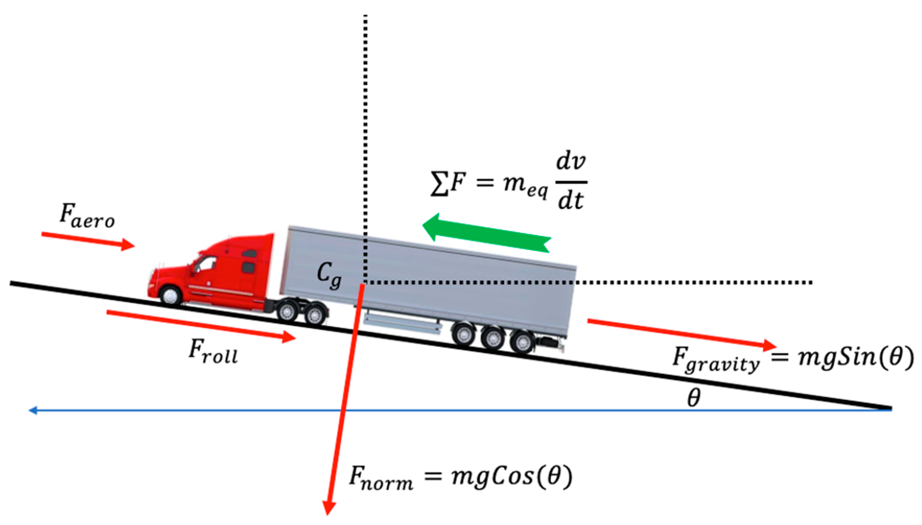
2.5. Force Balance
The different forces at the wheel are summed up and then divided by the equivalent vehicle mass to obtain the acceleration. Finally, the acceleration is integrated to obtain the velocity of the vehicle, which is used to feed back to the upstream controllers for a full closed loop dynamic. Figure 2 shows the different forces acting on the vehicle.
The gravitational force as a function of the road grade is given by Equation (2).
where, θ is the road grade in radians and m is the mass of the vehicle in kg and g is the gravitational acceleration in .
The aerodynamic drag is a direct function of vehicle speed and is given by Equation (3).
where, is the vehicle frontal area, is the drag coefficient and is the air density.
The road normal force is a function of road grade and is given by Equation (4).
where, is the road grade in radians.
Hence, using Newton’s second law for force balance principle and rearranging, the vehicle speed is given by Equation (5).
The optimal problem is solved in the distance domain, as the time in this solution is not fixed. Depending on the speed modulation, the time for the entire route will change and, hence, the problem is changed from a fixed time problem to a fixed distance problem. Hence, we convert Equation (5) as
where, the initial condition of the integration is Equation (6)
where, is the initial velocity in distance domain and is the initial velocity in time domain.
It is worth noting here that Equation (6) makes vehicle speed a state of the system dynamics. The assumptions made throughout this section while designing the system dynamics are
- Rotational compliance and coupling dynamics between components are not considered for the purpose of this research.
- Losses are considered constant instead of a function of any dependent variables.
- Map-based logic is used in every calculation possible to eliminate the need of complex analytical design.
Since the research is based on energy level analysis, the above considerations are justified. Hence the five continuous states are vehicle speed, vehicle position, engine fuel quantity, battery SOC and battery temperature. There is also another state, which is the gear number, but this is a discrete integer state, hence the problem is a mixed integer non-linear type. The control inputs are engine throttle, clutch command, brake command, and gear shift request. Power split between the internal combustion engine and electrical energy storage is decided by a simple splitting logic where the battery does whatever it can, and the rest is provided by the engine. Similarly, for regeneration, the battery absorbs energy to its SOC-based limits and the rest is consumed by the engine as motoring torque.
3. Problem Approach
A multi-objective minimization problem is solved in this work for a mixed integer type non-linear dynamical system. The objective is to achieve a fuel-efficient solution based on “a-priori” knowledge of the road elevation for the entire route. Since better fuel-efficient operation also indicates a better engine operating point in the brake thermal efficiency (BTE) contours, we also anticipate improving the emission. The reduced-order vehicle dynamical model, as described in the above section, is used to solve the problem using four individual control levers. The controls are cruise set speed, clutch disengagement with engines either ON or OFF, dynamic gear shift and dynamic torque split (splitting power between engine and battery). A weighted sum of total fuel consumed, and total trip time is used as the cost function. Rate of change of battery temperature is the third objective in the cost function to assure that the battery is operating in its most optimal operating zone. Equation (8) shows the cost function.
where, is the fuel rate, is the vehicle speed, α is the tuning coefficients for fuel consumed and trip time, are normalizing weights to transform the units in the same domain and ∆x is the integration step in distance domain. is the rate of change of battery internal temperature and β is the independent tuning weight. The dynamics in time domain are converted to distance domain by dividing the differential equations by vehicle speed (v(s)). Inclusion of time in the cost function is a measure of drivability. It is not acceptable to achieve a fuel-efficient solution if the time constraints are not met. In other words, the vehicle cannot take more time to cover the route, to save fuel and emissions.
Figure 3 shows the high-level architecture of the problem. The platooning problem is solved by the authors in another paper in a two-step problem approach. In this work, only the offline optimizer part of the problem is solved, as detailed in the below sections. The look-ahead road grade is fetched from the corridor information module, where it is assumed that the full route information is available. Now that we know the details of the problem and how we are going to approach those, we will lay down the individual problem in some more details. There are four control factors in this work which are implemented in a cascaded approach by introducing one control parameter at a time and then finally solving the problem with all the control parameters. The problem has five states x(.) = [vehicle speed, transmission gear number, clutch state and battery SOC and temperature], and four controls u(s) = [throttle, clutch command, gear shift command, power split ratio]. Engine speed is another derived state which is not explicitly needed by dynamic programming. Position in the route is another exogenous state which is used in the optimal model. Constraints that are modelled in this work are both soft and hard. Vehicle speed is limited between an absolute maximum and minimum threshold as a hard constraint. A soft root mean square type, second order norm constraint is also used, which is based on the difference between baseline speed profile and the optimal speed profile. Additional constraints for the coast problem are the duration and frequency of coast events. Since the predictive behavior can increase or decrease the vehicle speed from the cruise set speed, it is required to appropriately set constraints on vehicle speed. Similarly, the engine-off coast can also increase speed beyond reasonable limits if not monitored correctly. Hence, there are vehicle and engine speed limits set up accordingly while solving the problem.
Dynamic Program Formulation
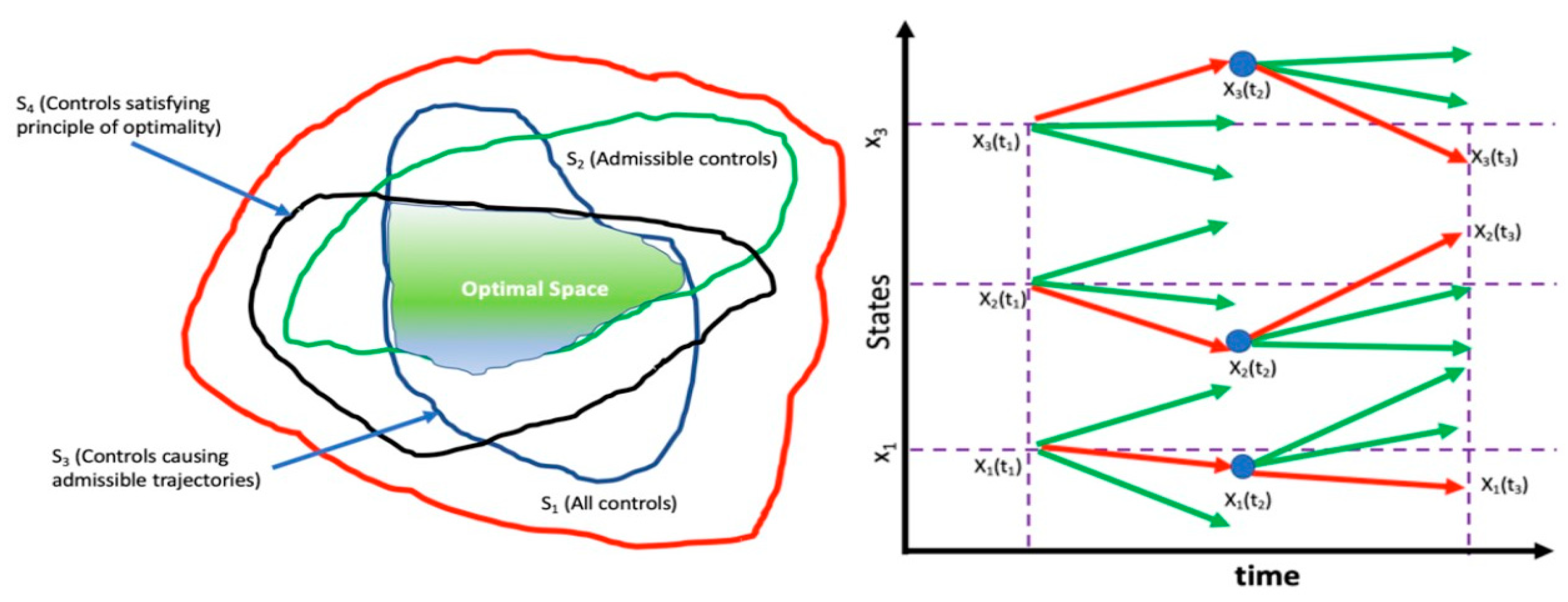
The problem is solved using dynamic programming and backtracking the cost, which is a potential solver for accurately solving global optimal problems with non-linear system dynamics. A dynamic programming-based control problem is well established by Guzella et al. [37,38,39]. Since dynamic programming has knowledge of the complete route and solves the problem in a backward fashion, it is guaranteed to provide a global optimal solution. Figure 4 shows the cost-to-go calculation and the selection of control variables. The iteration starts from the end as per the dynamic programming principle [40,41]. Starting from the end of the route, the cost is calculated at each position step, which in our work is set up to be 20 m, which is selected based on a resolution study for the optimization. It is also worth noting that 20 m corresponds to 0.7 s at 65 mph isochronous speed. This gives a good resolution for capturing any vehicle dynamics in terms of finding the optimal solution. The corresponding control levers are chosen at each position step, for which the calculated cost is minimum. The output of this solver is the optimal value for throttle, clutch, power split and gear shift. This throttle control is used as input to the closed loop system to generate the optimal speed profile using a model predictive controller. At each step, the minimum cost is obtained and added to the cost-to-go value for the forward closed loop control.
4. Detailed Problem and Subsequent Simulation Results
In this section, the individual control levers are formulated one at a time and then with each subsequent problem one additional control is added. This setup helps us to understand the problem better and the contribution and interaction of each added control factor. The route profile chosen for this work is an 86-mile-long section of I64 which has a good combination of road grade distribution.
4.1. Dynamic Speed Management
The first control lever used is cruise set speed. The idea here is to dynamically modulate the cruise set speed around 65 mph isochronous speed as a function of future road grade knowledge. This is like adaptive cruise control but is based on road grade information. Equation (9), shows the cost function as defined earlier,
subject to,
and, non-linear constraints,
There are four states here:
- 1 control input:
- u(s) = Throttle
- The primary output y(s) = [optimal vehicle speed target trajectory.
The search space is discretized between a minimum and maximum set of points for all these states. Engine speed is also a state, but it is a dependent state of the vehicle speed and hence it is not needed by the solver for the control problem. The engine speed is given by Equation (12),
where, is engine speed in is “gear ratio”, RAR is rear axle ratio and is wheel radius. Total time is included in the objective cost to make sure that total time remains within baseline limits. So, if the truck without predictive control takes “X” seconds to cover the route, the optimal control should also be close to that “X” seconds. The output of this solver is the optimal throttle value. This throttle control is used as input to the closed loop system to generate the optimal speed profile based on traditional model predictive control. The vehicle will no longer target a constant 65 mph cruise set speed in this case, as the optimal throttle will let the vehicle dynamically increase speed and slowdown in the route based on look-ahead grade information. Since dynamic programming with backtracking is computationally heavy, parallel computation using a multi-core system is used wherever possible. One such situation is when the stage cost is calculated for discretized points. During this step, the full set of points is divided into smaller sets and the problem is solved for those smaller sets in different cores of the system CPU. Table 3 shows the key metrics for the cruise speed modulation problem. It shows an absolute fuel economy of 3.02% with a change of 0.07% in trip time. There is a reduction of 1% of aerodynamic work and 2.56% reduction in total cycle work. The brake thermal efficiency improved by 0.18%. Negative work reduction is mostly due to engine braking reduction. The % improvement numbers are against the baseline simulation where the vehicle cruise set speed is 65 mph.
A key observation from this problem is that the predictive cruise control modulates speed around uphill and downhill areas. Specifically, it increases speed before going uphill and decreases speed before going downhill. In the energy domain, it is like gaining energy when it is easy in the flat section and then utilizing the kinetic energy gained to cover the uphill section to overcome the grade drag. Similarly, during the downhill section, it is efficient to slow down a bit before going downhill to save energy (fuel), since speed is expected to increase going downhill while having to brake, thereby wasting energy which is gained at the expense of fuel. The main objective here is to reduce the negative work in the form of reduced engine braking. Speed modulation during the 283 flat sections are not very common. During the flat section, the truck follows the usual route 284 speed limit, which is 65 mph or 29 m/s in this work. Emissions are also improved as a passive component due to the engine operating point change. Now that the engine operates at a better BTE zone consuming less fuel, we observe a better NOx number. The normalized NOx reduction from the baseline simulation is around 5% in this optimal problem formulation.
4.2. Dynamic Speed and Coast (Engine Idle + Engine Off) Management
The vehicle dynamics and the cost function for this problem is like what is used for speed management. An additional state and control parameter is added to the speed problem. To manage coast, we need to know the current clutch state and then command the clutch to engage or disengage. One additional constraint here is the duration and frequency of coast events. Even though speed constraints will take care of how long coast events can be, there is a need for a constraint on how frequent the coast events could be. Hence, a penalty on the frequency of clutch state change is added. This will prevent frequent coast events and thereby reduce oscillations in operation. Table 4 shows the metrics for the problem, where only coasting is used as a control lever. A total of 1.3% compensated fuel savings is achieved by using the coast problem in the engine-off mode and around 0.9% by keeping the engine on while coasting. Most of the benefit is achieved by the reduction of cycle work, aerodynamic work, and a reduction in negative work. There is a reduction of engine out NOx in the order of 1.8% for both the engine-on and engine-off coasting scenarios. The difference in NOx reduction is not significant since the engine is tuned for ultra clean performance.
Table 5 shows the key energy domain metrics for the speed and coast problem together for the entire I64 portion of the route. This metric indicates that the negative work done is equivalent to the loss in kinetic energy of the vehicle which is gained at the expense of either fuel or electric energy. Since dynamic programming did not show the reason why the fuel benefits are occurring it is important to compare the reduction in negative work which clearly indicates where the fuel economy is coming from, along with the improvement in engine BTE. Analyzing the distributed speed and coast problems alone, it is evident that when speed and coast problems are solved together the fuel-saving benefits are additive. The speed and coast problem solved together achieved 3.6% for the engine idle coast case and 4.4% for the engine-off coast scenario. It is also worth noting that the engine-off case benefits are also additive.
Figure 5 shows the time domain evolution of various signals for the optimal problem. The plot shows a section of the I64 route. Subplot 2 shows the gear number for the two scenarios, and it shows near similar behavior which indicates similar engine operating conditions in the torque curve. Subplot 3 shows the difference in the vehicle speed for the two different problems along with the reference speed target generated by the optimal solver. Subplot 6 shows the grade power for the two optimal problems (engine off and engine idle). The plots are identical, as expected since the grade is same for the two problems. Subplot 7 in Figure 5 shows that the coast zones for the engine-off problem are not exactly like the coast zones for the engine idle problem. This indicates that predictive coast with engine-off and engine idle are two separate problems in terms of optimality. The black vertical boxes highlighted are the difference in behavior between the two problems.
4.3. Dynamic Speed, Coast (Engine Idle + Engine Off) and Gear Management
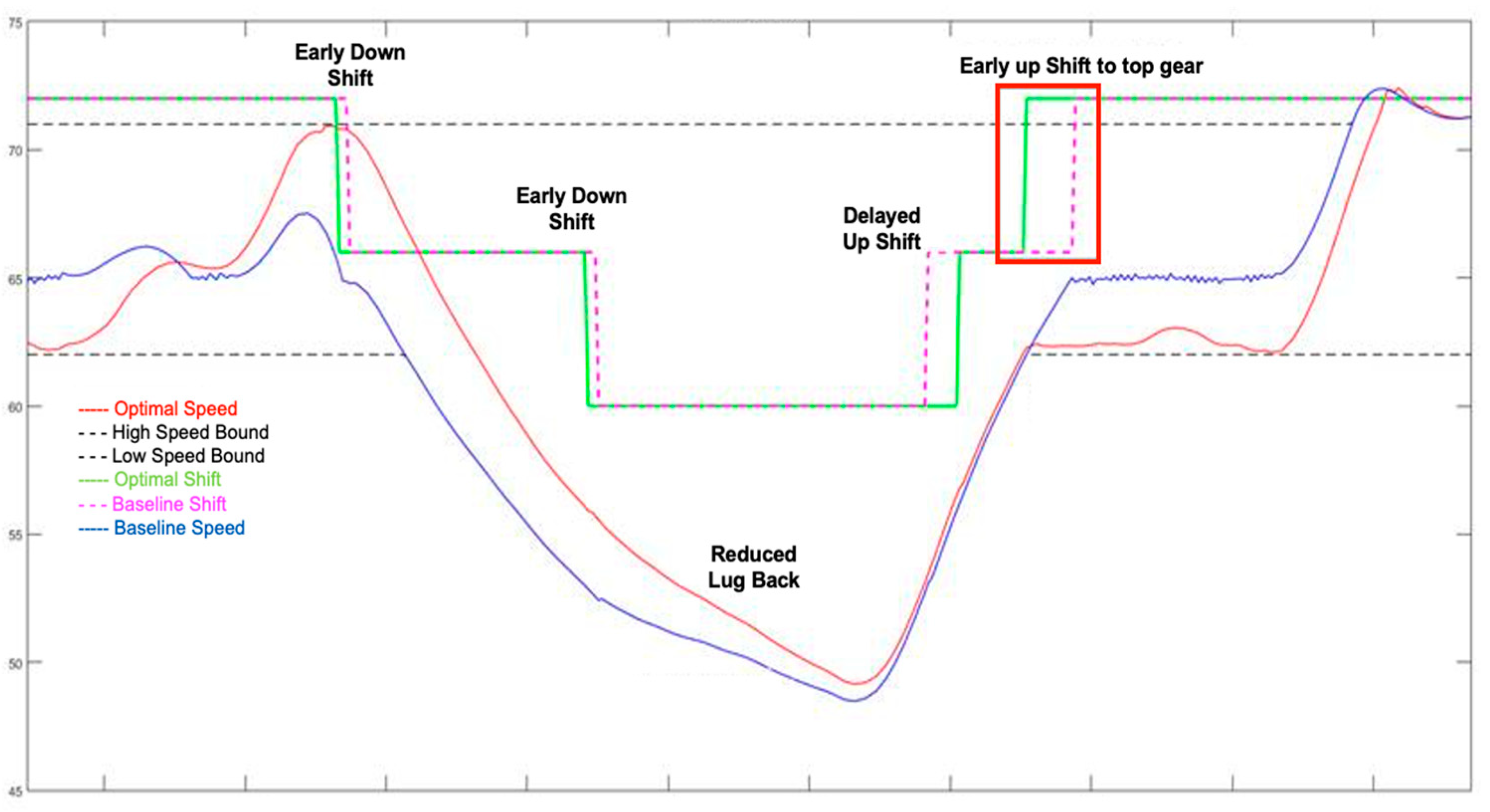
In this third problem, we have included predictive gear control as a third lever along with speed and coast controls. The objective function remains the same, with the addition of an extra control input which is the gear shift command. Gear shift command can take three possible states (up shift, hold gear and down shift). The objective here is to find if shifting the gear with the knowledge of road grade in the route will help achieve any fuel benefits and/or drivability improvements. Analytically, it is not expected to gain fuel benefits unless the fuel maps are tuned to include high brake thermal efficiency (BTE) zones for lower gears. It is also worth pointing out here that the engine efficiency maps used for this work have their peak BTE zones around a range of engine speed which corresponds to the top gear ratio of the transmission system. This means that if going down to a lower gear, the system will compromise on fuel savings. Hence, to achieve the minimum cost of fuel savings, the system will not down shift. This is also seen with the optimal solution. This problem did not provide any fuel benefits but neither did it penalize fuel savings. It was a hard problem to tune for, achieving at least the same fuel economy as with the previous problem, and with this tuning it is observed that the system down shifts a little early while in positive grade and stays at a lower gear a little more after coming out of positive grade. The interaction between gear shift for this problem and clutch disengagement for the coasting problem is handled through the addition of appropriate penalties. On the performance side, it is observed that with dynamic gear shifts the truck was able to maintain a higher speed in the uphill sections. This is illustrated in Figure 6. The red plot is the vehicle speed for the optimal solution, and it shows clear reduction in lug-back in the uphill section.
Table 6 shows the metrics for this problem with engine idle coasting as well as engine-off coasting. As discussed earlier, we notice insignificant improvement in compensated fuel economy. There is less engine out NOx reduction as compared to the coast only problem. This is due to the increase in lower gear operation. The impact of NOx improvement is not at all substantial to justify that addition of predictive knowledge for gear management can improve NOx production in the system. In fact, for some tuning cases, it increased the NOx production a bit due to the gear operation at a lower gear. This is analytically justified as well, since a lower gear operation means better performance rather than a better BTE zone operation. The good observation is that even with the fuel-efficient tuning for the optimal parameters it did not penalize NOx production drastically.
4.4. Dynamic Speed, Coast (Engine Idle + Engine Off), Gear and Torque (Power Split) Management
Lastly, the problem is solved for dynamically varying torque demand between the engine and battery system. This is calculated based on the predictive knowledge of the road grade and the battery system temperature. Analytically, it is not expected to provide significant fuel savings since the electrification system is quite limited in power. In this problem, there are no additional states involved but there is an extra control input for the dynamic solver. This new control input is power split ratio. The way this ratio is defined in the problem is by discretizing the entire hybrid power range including the charge and discharge limits. Hence, the electric power range of −20 kW to +20 kW, is discretized with equal grid size. The resolution of the grid size matters since it impact the results based on how dynamic and responsive the control input is.
Table 7 shows the key metrics for this problem. As discussed earlier, there are no substantial increases in fuel benefits. Figure 7 shows the total time spent in each gear for the individual problems. The plot enumerations are Bsln: no optimal behavior, VS: dynamic speed, VSC: dynamic speed and coast, VSG: dynamic speed and gear, VSCG: dynamic speed, coast, and gear, VSCGP: dynamic speed, coast, gear, and power split. These metrics provides an understanding of which gear is predominantly being exercised by each problem. Since downshifting to a lower gear will take the operation outside of the maximum BTE zone, it is not expected that the gear problem will try to shift down for a better fuel-efficient solution. Hence, for this kind of BTE map a more fuel-efficient solution is practically not possible. The gear problem can expect to provide a better drivability by helping to reduce lug backs on a steep hill. It is seen in Figure 7 that all the problem types are trying to increase top gear operation since fuel saving will be more due to the BTE contour positioning. It is also interesting to observe that the problem with gear management is reducing the time in (top-1) gear. The coast management problem alone is the only problem which is not able to increase top gear operation much as compared to the other problems. This is because with the coast management problem, since the vehicle is not predictively modulating speed and gear, the speed drops are more which causes the gear to shift down more.
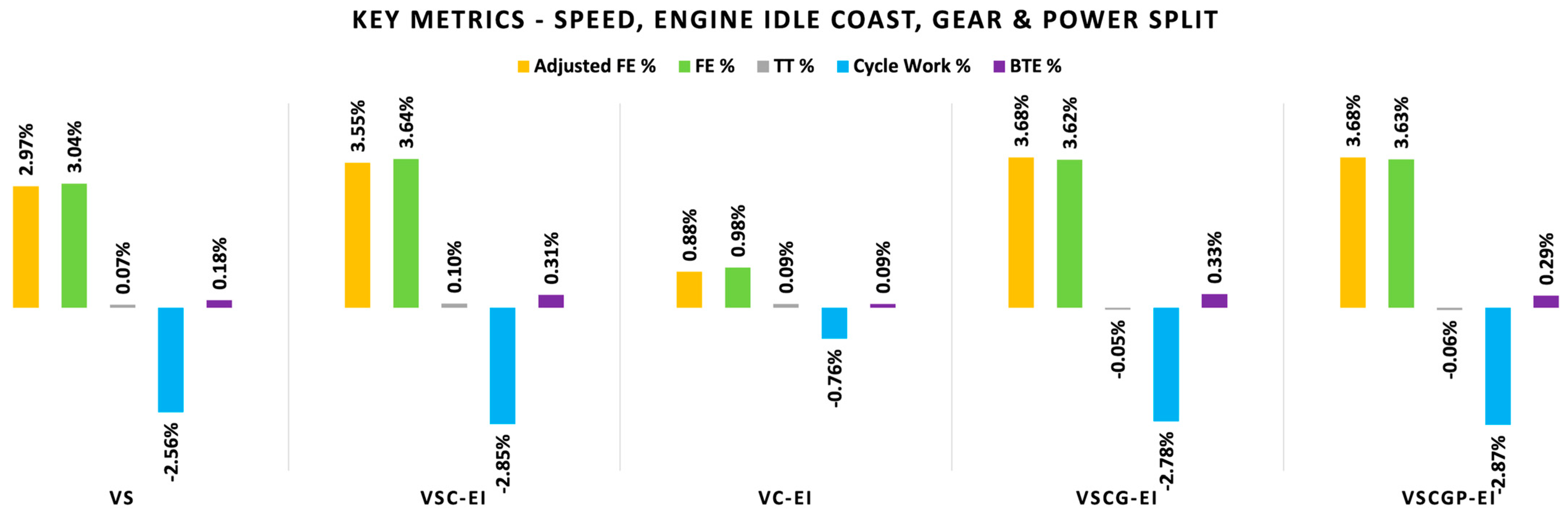
Figure 8 shows the key metrics for the complete problem with the engine idle coasting condition. The plot shows the absolute fuel economy for each problem when compared to the baseline case. The orange plot is the % change in trip time. The green plot is a measure of relative fuel economy which is the difference between the absolute fuel economy and the % change in trip time. This is to make sure that negative trip time is compensated accordingly. The plots also shows the reduction in cycle work and the improvement in brake thermal efficiency in each case. Figure 9 shows the reduction in aerodynamic drag and the reduction in engine out NOx numbers. The complete problem achieved a 3.7% fuel economy and a NOx reduction of 8.3%. The corresponding BTE improvement in this case is much lower and is close to 0.3%.
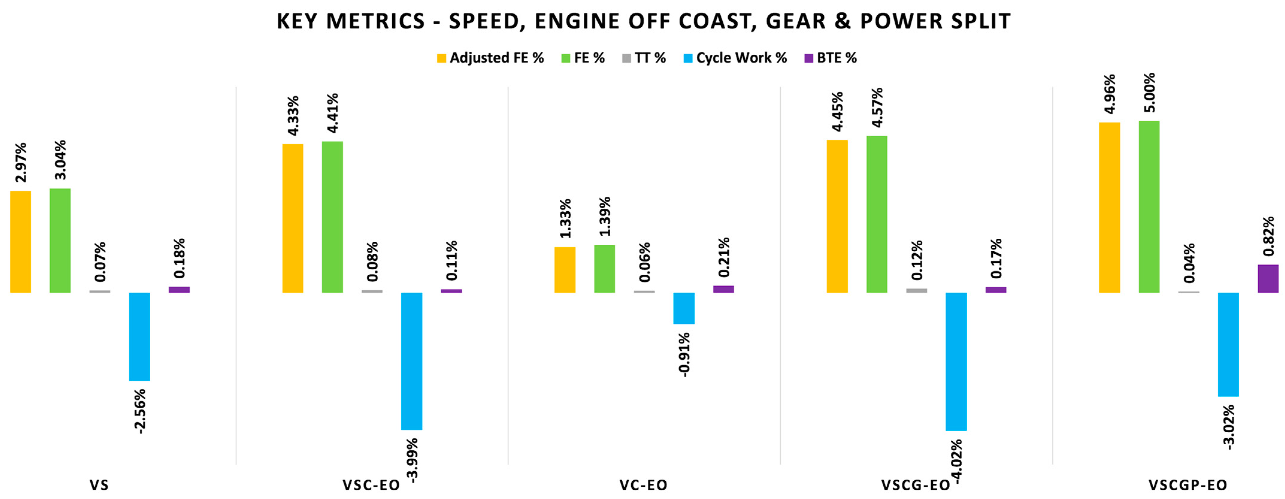
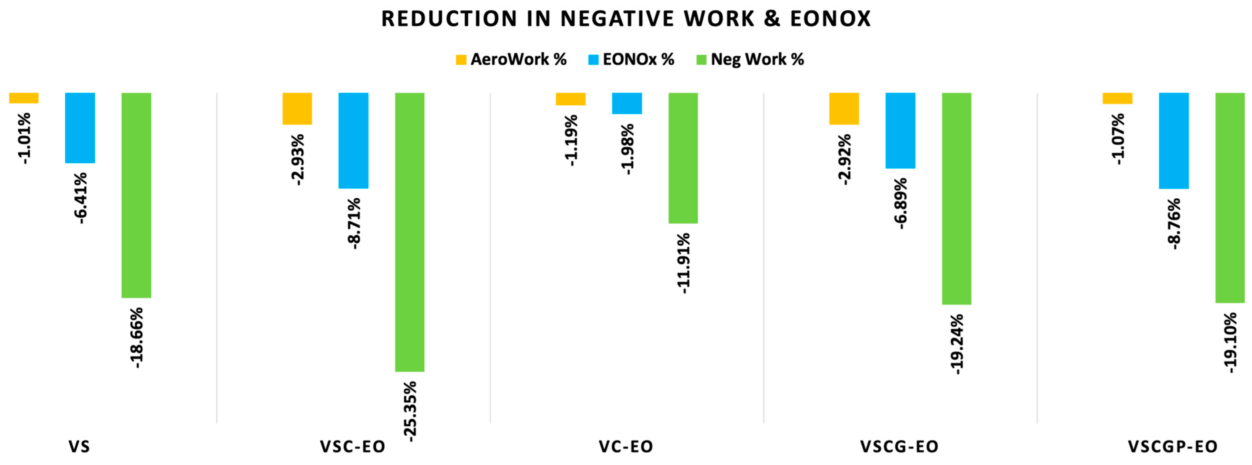
Figure 10 and Figure 11 captures the detailed metrics for all the problems stacked up for the engine-off coasting case. Overall, an impressive 5% fuel economy is achieved with the predictive features working together with engine-off coasting condition. This benefit is mostly contributed by 0.8% improvement in BTE, 3% reduction in cycle work and 19% reductions in negative work. There is also an associated NOx reduction with each control lever. NOx reduction was 8.75%. This is because engine BTE has improved.
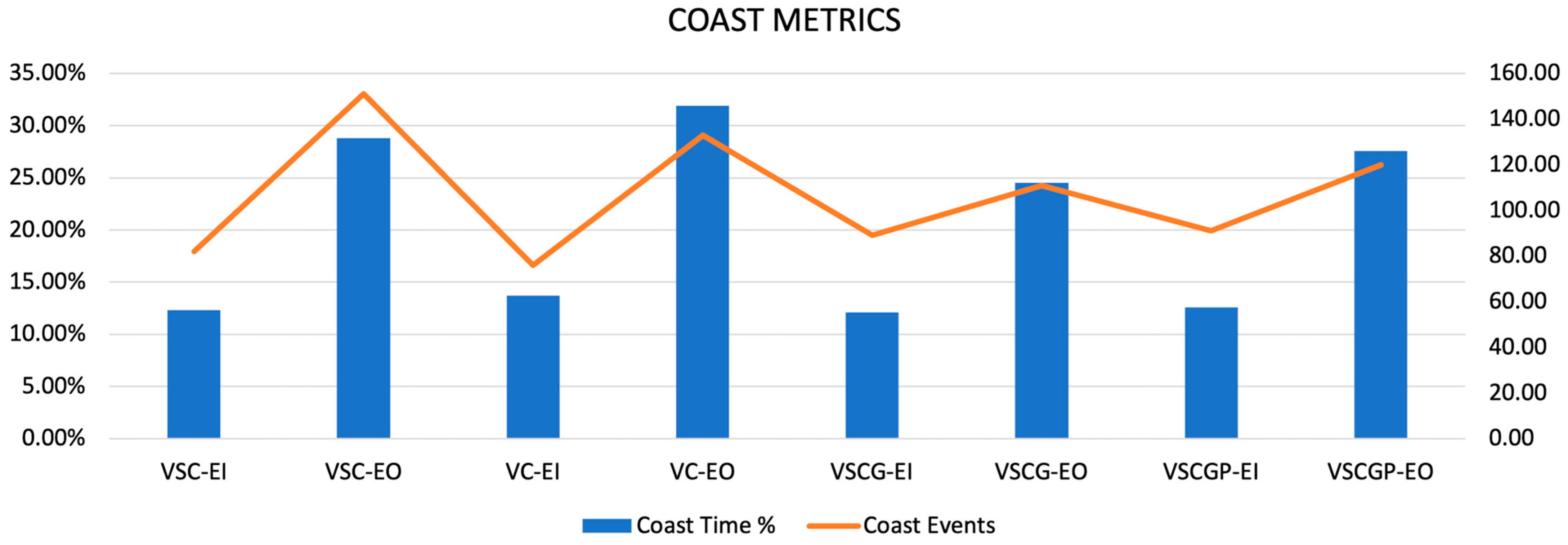
Figure 12 shows the coast metrics for various problems. The bars show the percentage of time in coast by each problem and the line plot shows the number of coast events in each problem. Engine-off and engine idle coast metrics show similar behavior in terms of time in coast and number of coast events. Interestingly, the coast alone problem has a good amount of coasting events but could not provide a lot of benefit, simply because the net fuel economy is not related to coast events alone but is a combined factor of multiple scenarios including cycle work reduction, negative work reduction, BTE improvements and aerodynamic drag reduction. Further, a couple of very large coast events were also observed which may not be feasible in the real environment due to physical engine operation restrictions. Nevertheless, the metric gives an overview of the coast event distribution across various problem sets.
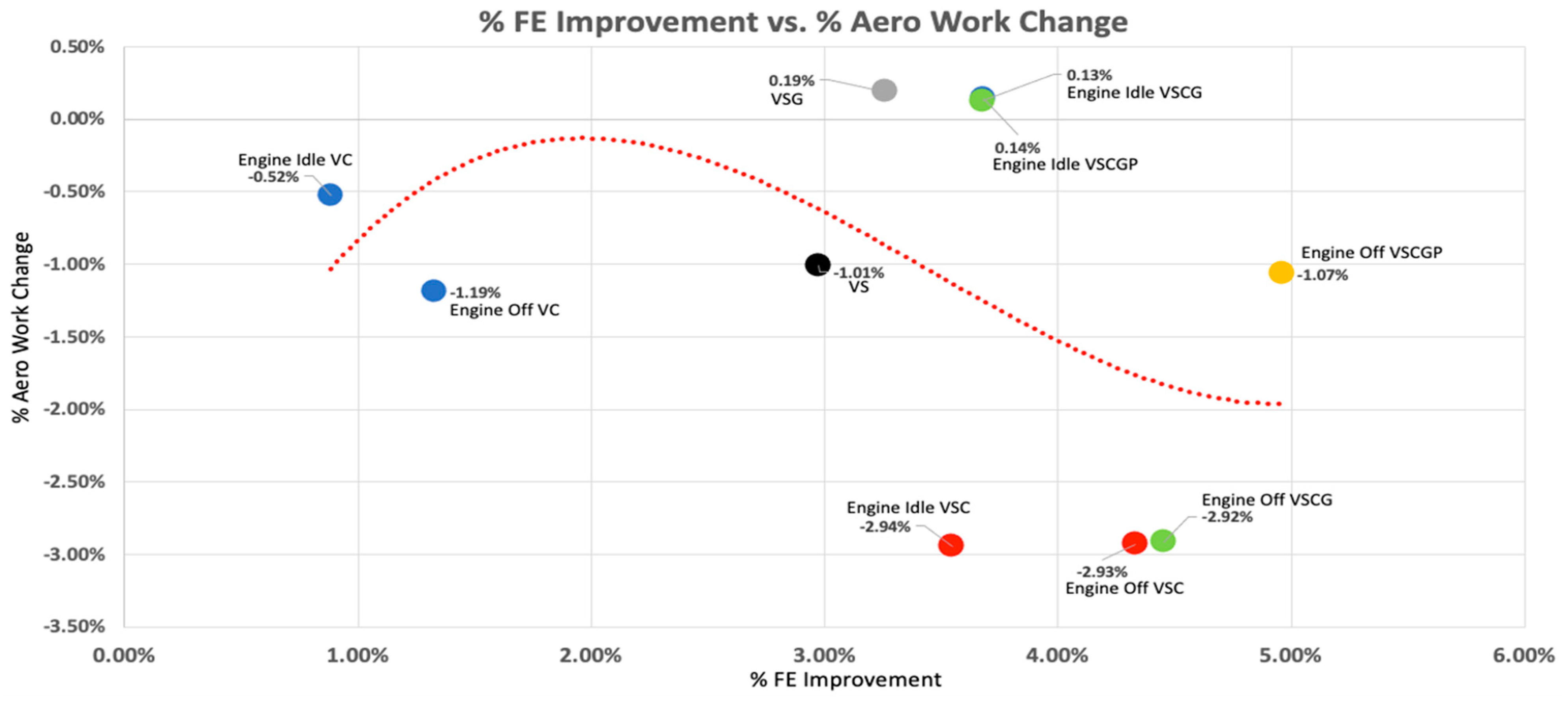
Figure 13 shows the % change in aerodynamic work as a function of % improvement in fuel economy. There is no concise correlation between the two in terms of the different problems. This is because the trip time is balanced with baseline trip time. Hence, the overall increase/decrease in speed tends to balance each other. The dynamic speed coast problem shows typically more aerodynamic work reduction. This is because they are only slowing down the vehicles whenever possible by going to coasting, along with speed modulation.
Figure 14 shows similar trends as compared to the cycle work reduction. It shows the metric is correlated to speed modulation. Since negative work is due to the speed band operating at regions beyond the engine braking limits, with the coast-alone problem, vehicle speed is not intentionally modulated to a higher or lower value at the expense of the fuel, hence the reduction is less as compared to the baseline results. In this case, the speed modulation typically follows the baseline numbers. The other problems have a lesser spread with the engine idle problem as compared to the engine-off problem. It is noted that there is a linear trend in fuel economy and negative work reduction for all problems except the problems with the addition of the gear modulation.
Figure 15 shows the reduction in total cycle work of the engine because of the predictive knowledge of the road grade. The bubbles shows the reduction in engine out NOx as a function of the reduction in % cycle work by the engine. Though it can also be seen that the reduction is more in case of an engine-off case, which is because the engine idle work is taken away in this case. In case of the engine idle scenario, the reductions for all the problems are around −2.75% while the problem with engine idle coast only is around −0.76%, while with the engine-off scenario, the problems with vehicle speed along with coast, gear and power split provides added reduction, as compared to the vehicle speed alone problem only. This clearly demonstrates the fact that the problem with engine idle and engine-off cases are completely different in behavior and cannot be determined by interpreting zero fuel consumption by engine idle problem during the idle sections. This is an important observation. Similar trends are also observed with the negative work reduction for both the engine-off and engine idle coast cases. Negative work in this case is comprised of engine braking work and motoring work.
Similarly, Figure 15 shows the variation of cycle work reduction to brake thermal efficiency (BTE) improvement. There is no strong correlation between the problems and the general behavior. Another quick analysis done in this work is to run the same problem on a shorter section of the route. This was done to understand the look-ahead distance required for optimal behavior. The complete route is divided into two sections of 40 miles each, one for the first half and the next for the second half. Table 8 shows the % fuel economy numbers for the two sections of the route.
The results from Table 8 shows that the overall behavior and fuel economy numbers stay near similar if we shorten the route to half. Since the route is not exactly symmetrical the numbers are not equally divided. The coast events also reduced a little for the first half of the route and increased marginally for the second section. This is solely because the grade profile is not similar. It is also noted that the optimal control shows similar physical behavior during the very short hilly section where there were no coast events observed and the vehicle speed modulation was also not effective. The predictive gear played a role by reducing the lug back. It is noted that the fuel economy is not at all achieved in this section. While in the flat section, there is the usual behavior of coast events, and the problem was able to achieve around 1% benefit. There is also slowing down of the vehicle because there were coast events which slowed the speed down. Overall, if these results are compared with the full route solution it is not observed that the benefits are hugely sacrificed. Specifically, for the 40-mile route it is noted that the benefits are almost equally divided between the two segments and add up to achieve close to the full route benefits.
5. Conclusions and Further Work
This research indicates that predictively applying control action with a priori knowledge of the road grade can provide increased fuel economy without negatively impacting vehicle performance. Dynamic cruise and coast control provide most benefits, while predictively controlling gear and torque (power split) does not provide any significant fuel benefit but does offer improved drivability and powertrain efficiency. The major outcomes of the work are:
- Predictive road grade knowledge can help design control algorithms that will enable fuel savings depending on road grade profile
- Vehicle cruise speed can be increased within acceptable bounds (calibrated for drivability) before entering an uphill
- Vehicle cruise speed can be reduced within calibratable bounds before entering a downhill
- Down shift gear to a lower value predictively before hitting speed lug back travelling uphill
- Up shift gear predictively while still travelling uphill and before completely coming out of the hill
- Engine can be disengaged and turned off in mild down grade
- Engine can be disengaged for a short duration during the flat section of route with predictive speed modulation (increase speed then disengage)
This analysis is also a precursor to predictive platooning systems. The usage of this formulation in a platooning system is discussed in another paper by the same authors.
Author Contributions
Conceptualization, Methodology, Investigation and Validation—S.P. Review and Supervision—S.A. All authors have read and agreed to the published version of the manuscript.
Funding
This research received no external funding.
Institutional Review Board Statement
Not applicable.
Informed Consent Statement
Not applicable.
Data Availability Statement
Not applicable.
Conflicts of Interest
The authors declare no conflict of interest.
References
- Sun, X.; Cao, Y.; Jin, Z.; Tian, X.; Xue, M. An Adaptive ECMS Based on Traffic Information for Plug-in Hybrid Electric Buses. IEEE Trans. Ind. Electron. 2022, 1–10. [Google Scholar] [CrossRef]
- Guo, J.; Guo, Z.; Chu, L.; Zhao, D.; Hu, J.; Hou, Z. A Dual-Adaptive Equivalent Consumption Minimization Strategy for 4WD Plug-In Hybrid Electric Vehicles. Sensors 2022, 22, 6256. [Google Scholar] [CrossRef] [PubMed]
- Zecchi, L.; Sandrini, G.; Gadola, M.; Chindamo, D. Modeling of a Hybrid Fuel Cell Powertrain with Power Split Logic for Onboard Energy Management Using a Longitudinal Dynamics Simulation Tool. Energies 2022, 15, 6228. [Google Scholar] [CrossRef]
- Wang, Y.; Boggio-Marzet, A. Evaluation of eco-driving training for fuel efficiency and emissions reduction according to road type. Sustainability 2018, 10, 3891. [Google Scholar] [CrossRef] [Green Version]
- Scalarretta, A.; Serrao, L.; Dewangan, P.C.; Tona, P.; BergShoeff, E.N.D.; Bordons, C.; Hubacher, M.; Isenegger, P.; Lacandia, F.; Laveau, A.; et al. A control benchmark on the energy management of a plug-in-hybrid electric vehicle. Control Eng. Pract. 2014, 29, 287–298. [Google Scholar] [CrossRef] [Green Version]
- Nilsson, M.; Johannesson, L.; Askerdal, M. ADMM Applied to Energy Management of ancillary systems in truck. In Proceedings of the 2015 American Control Conference (ACC), Chicago, IL, USA, 1–3 July 2015; pp. 3459–3466. [Google Scholar]
- Huang, Y.; Wang, H.; Khajepour, A.; He, H.; Ji, J. Model predictive control power management strategies for HEV’s. Rev. J. Power Sources 2017, 341, 91–106. [Google Scholar] [CrossRef]
- Biral, F.; Bertolazzi, E.; Bossetti, P. Notes on numerical methods for solving optimal control problem. IEEE J. Ind. Appl. 2016, 5, 154–166. [Google Scholar] [CrossRef] [Green Version]
- Gao, Z.; LaClair, T.; Ou, S.; Huff, S.; Wu, G.; Hao, P.; Boriboonsomsin, K.; Barth, M. Evaluation of electric vehicle component performance over eco-driving cycles. Energy 2019, 172, 823–839. [Google Scholar] [CrossRef]
- Xu, Y.; Li, H.; Liu, H.; Rodgers, M.O.; Guensler, R.L. Eco-driving for transit: An effective strategy to conserve fuel and emissions. Appl. Energy 2017, 194, 784–797. [Google Scholar] [CrossRef]
- Terwen, S.; Back, M.; Krebs, V. Predictive Powertrain Control for Heavy Duty Trucks. IFAC Proc. Vol. 2004, 37, 105–110. [Google Scholar] [CrossRef]
- Kirches, C.; Bock, H.G.; Schlöder, J.P.; Sager, S. Mixed-integer NMPC for predictive cruise control of heavy-duty trucks. In Proceedings of the 2013 European Control Conference (ECC), Zurich, Switzerland, 17–19 July 2013; pp. 4118–4123. [Google Scholar] [CrossRef]
- Hellström, E. Explicit use of road topography for model predictive cruise control in heavy trucks. Technology. 2005. Available online: https://www.diva-portal.org/smash/record.jsf?pid=diva2%3A20186&dswid=7919 (accessed on 7 January 2022).
- Johannesson, L.; Murgovski, N.; Jonasson, E.; Hellgren, J.; Egardt, B. Predictive energy management of hybrid long-haul trucks. Control Eng. Pract. 2015, 41, 83–97. [Google Scholar] [CrossRef]
- Borek, J.; Groelke, B.; Earnhardt, C.; Vermillion, C. Optimal Control of Heavy-duty Trucks in Urban Environments through Fused Model Predictive Control and Adaptive Cruise Control. In Proceedings of the 2019 American Control Conference (ACC), Philadelphia, PA, USA, 10–12 July 2019; pp. 4602–4607. [Google Scholar] [CrossRef]
- Kock, P.; Gnatzig, S.; Passenberg, B.; Stursberg, O.; Ordys, A. Improved Cruise Control for Heavy Trucks using combined Heuristic and Predictive Control. In Proceedings of the IEEE International Conference on Control Applications, CCA 2008, San Antonio, TX, USA, 3–5 September 2008. [Google Scholar]
- Li, X.; Lyu, J.; Hong, J.; Zhao, J.; Gao, B.; Chen, H. MPC-Based Downshift Control of Automated Manual Transmissions. Automot. Innov. 2019, 2, 55–63. [Google Scholar] [CrossRef]
- Khodabakhshian, M.; Feng, L.; Börjesson, S.; Lindgärde, O.; Wikander, J. Reducing auxiliary energy consumption of heavy trucks by onboard prediction and real-time optimization. Appl. Energy 2017, 188, 652–671. [Google Scholar] [CrossRef]
- Groelke, B.; Borek, J.; Earnhardt, C.; Li, J.; Geyer, S.; Vermillion, C. A Comparative Assessment of Economic Model Predictive Control Strategies for Fuel Economy Optimization of Heavy-Duty Trucks. In Proceedings of the 2018 Annual American Control Conference (ACC), Milwaukee, WI, USA, 27–29 June 2018; pp. 834–839. [Google Scholar] [CrossRef]
- Fries, M.; Kruttschnitt, M.; Lienkamp, M. Operational Strategy of Hybrid Heavy-Duty Trucks by Utilizing a Genetic Algorithm to Optimize the Fuel Economy Multiobjective Criteria. IEEE Trans. Ind. Appl. 2018, 54, 3668–3675. [Google Scholar] [CrossRef]
- Junell, J.; Tumer, K. Robust predictive cruise control for commercial vehicles. Int. J. Gen. Syst. 2013, 42, 776–792. [Google Scholar] [CrossRef]
- Borek, J.; Groelke, B.; Earnhardt, C.; Vermillion, C. Economic optimal control for minimizing fuel consumption of heavy-duty trucks in a highway environment. IEEE Trans. Control. Syst. Technol. 2020, 28, 1652–1664. [Google Scholar] [CrossRef]
- Xie, S.; Lang, K.; Qi, S. Aerodynamic-aware coordinated control of following speed and power distribution for hybrid electric trucks. Energy 2020, 209, 118496. [Google Scholar] [CrossRef]
- Khodabakhshian, M.; Feng, L.; Wikander, J. Predictive control of the engine cooling system for fuel efficiency improvement. In Proceedings of the 2014 IEEE International Conference on Automation Science and Engineering (CASE), New Taipei, Taiwan, 18–22 August 2014; pp. 61–66. [Google Scholar] [CrossRef] [Green Version]
- Zeng, Y.; Cai, Y.; Kou, G.; Gao, W.; Qin, D. Energy management for plug-in hybrid electric vehicle based on adaptive simplified ECMS. Sustainability 2018, 10, 2060. [Google Scholar] [CrossRef] [Green Version]
- Rezaei, A.; Burl, J.B.; Zhou, B.; Rezaei, M. A New Real-Time Optimal Energy Management Strategy for Parallel Hybrid Electric Vehicles. IEEE Trans. Control. Syst. Technol. 2019, 27, 830–837. [Google Scholar] [CrossRef]
- Tian, X.; Cai, Y.; Sun, X.; Zhu, Z.; Xu, Y. An adaptive ECMS with driving style recognition for energy optimization of parallel hybrid electric buses. Energy 2019, 189, 116151. [Google Scholar] [CrossRef]
- Lithium-Ion 48V Battery. Version October 11. 2022. Available online: https://www.a123systems.com/automotive/products/systems/48v-battery/ (accessed on 7 January 2022).
- X15 Efficiency Series. 2020. Available online: https://www.cummins.com/engines/x15-efficiency-series (accessed on 21 April 2020).
- P2 Off-Axis Module for Hybrid Vehicles. BorgWarner P2 Off Axis Module. Available online: https://cdn.borgwarner.com/docs/default-source/default-document-library/p2-off-axis-module-for-hybrid-vehicles.pdf?sfvrsn=2ba5b43c_18 (accessed on 8 January 2022).
- Afzal, A.; Kaladgi, A.R.; Jilte, R.; Ibrahim, M.; Kumar, R.; Mujtaba, M.; Alshahrani, S.; Saleel, C.A. Thermal modelling, and characteristic evaluation of electric vehicle battery system. Case Stud. Therm. Eng. 2021, 26, 101058. [Google Scholar] [CrossRef]
- Chowdhury, S.; Leitzel, L.; Zima, M.; Santacesaria, M.; Lustbader, J.; Rugh, J.; Winkler, J.; Khawaja, A.; Govindarajalu, M. Total Thermal Management of Battery Electric Vehicles (BEVs). In Proceedings of the CO2 Reduction for Transportation Systems Conference; SAE International: Warrendale, PA, USA, 2018. [Google Scholar] [CrossRef] [Green Version]
- Chang, W.Y. The State of Charge Estimating Methods for Battery: A Review. ISRN Appl. Math. 2013, 2013, 953792. [Google Scholar] [CrossRef] [Green Version]
- Zhang, M.; Fan, X. Review on the state of charge estimation methods for electric vehicle battery. World Electr. Veh. J. 2020, 11, 23. [Google Scholar] [CrossRef] [Green Version]
- Ng, K.S.; Moo, C.S.; Chen, Y.P.; Hsieh, Y.C. Enhanced coulomb counting method for estimating state-of-charge and state-of-health of lithium-ion batteries. Appl. Energy 2009, 86, 1506–1511. [Google Scholar] [CrossRef]
- Endurant HD Automated Transmission. Available online: https://www.eatoncummins.com/us/en-us/catalog/transmissions/endurant.specifications.html (accessed on 22 April 2020).
- Pan, Y.; Theodorou, E. Probabilistic differential dynamic programming. Advances in Neural Information Processing Systems; Curran Associates, Inc., 2014; pp. 1907–1915. Available online: https://proceedings.neurips.cc/paper/2014/file/7fec306d1e665bc9c748b5d2b99a6e97-Paper.pdf (accessed on 8 January 2022).
- Larsson, V.; Johannesson, L.; Egardt, B. Cubic spline approximations of the dynamic programming cost-to-go HEV energy management problems. In Proceedings of the in 2014 European Control Conference (ECC), Strasbourg, France, 24–27 June 2014; pp. 1699–1704. [Google Scholar]
- Romijin, C.; Donkers, T.; Weiland, S.; Kessels, J. Complex vehicle energy management with large horizon optimization. In Proceedings of the 34 Benelux Meeting on Systems & Controls, Osaka, Japan, 15–18 December 2015. [Google Scholar]
- Smith, D.K. Dynamic Programming and Optimal Control. Volume 1. J. Oper. Res. Soc. 1996, 47, 833–834. [Google Scholar] [CrossRef]
- Bellman, R.E.; Dreyfus, S.E. Applied Dynamic Programming; Princeton University Press: Princeton, NJ, USA, 2015. [Google Scholar] [CrossRef]

Figure 2.
1D longitudinal forces on a vehicle.

Figure 3.
Overview of the problem architecture.

Figure 4.
Illustration of dynamic programming solver.

Figure 5.
Performance results for optimal solution compared to baseline rule based control. The plot is a zoomed version of a stitched version of different sections in the route.
Figure 5.
Performance results for optimal solution compared to baseline rule based control. The plot is a zoomed version of a stitched version of different sections in the route.

Figure 6.
Predictive optimality in gear management. The problem shows the predictive gear shift.

Figure 7.
% Time in top 4 gears for each DOE. The comparison must be between the top 2 gears. Predictive gear tries to operate more at a lower gear while fuel economy tends to operate at a higher gear.
Figure 7.
% Time in top 4 gears for each DOE. The comparison must be between the top 2 gears. Predictive gear tries to operate more at a lower gear while fuel economy tends to operate at a higher gear.

Figure 8.
Key metrics showing the comparison of benefits along with cycle work and BTE for the complete set of problem including speed, coast, gear, and power split management. This scenario is with engine idle coast.
Figure 8.
Key metrics showing the comparison of benefits along with cycle work and BTE for the complete set of problem including speed, coast, gear, and power split management. This scenario is with engine idle coast.

Figure 9.
Reduction in aerodynamic work along with associated EONOx reduction. The last bar plot shows the reduction in negative work which includes engine braking, motoring losses and service braking.
Figure 9.
Reduction in aerodynamic work along with associated EONOx reduction. The last bar plot shows the reduction in negative work which includes engine braking, motoring losses and service braking.

Figure 10.
Key metrics showing the comparison of benefits along with cycle work and BTE for the complete set of problems including speed, coast, gear, and power split management. This scenario is with engine-off coast.
Figure 10.
Key metrics showing the comparison of benefits along with cycle work and BTE for the complete set of problems including speed, coast, gear, and power split management. This scenario is with engine-off coast.

Figure 11.
Reduction in aerodynamic work along with associated EONOx reduction. The last bar plot shows the reduction in negative work which includes engine braking, motoring losses and service braking.
Figure 11.
Reduction in aerodynamic work along with associated EONOx reduction. The last bar plot shows the reduction in negative work which includes engine braking, motoring losses and service braking.

Figure 12.
Coast metrics for all combination of problems with coast formulation. The bars show the % time in coast for each problem and the plot shows the number of coast events.
Figure 12.
Coast metrics for all combination of problems with coast formulation. The bars show the % time in coast for each problem and the plot shows the number of coast events.

Figure 13.
% Change in aerodynamic work as a function of % fuel economy improvement for various optimal problem setups.
Figure 13.
% Change in aerodynamic work as a function of % fuel economy improvement for various optimal problem setups.

Figure 14.
% Reduction in negative work as a function of % fuel economy improvement for various optimal problem setups.
Figure 14.
% Reduction in negative work as a function of % fuel economy improvement for various optimal problem setups.

Figure 15.
% Change in brake thermal efficiency as a function of % change in cycle work for different combination of optimal problems.
Figure 15.
% Change in brake thermal efficiency as a function of % change in cycle work for different combination of optimal problems.


Table 1.
Transmission gear ratios [36].
Table 1.
Transmission gear ratios [36].
| Gear Type | Gear # | Gear Ratio |
|---|---|---|
| 1 | 14.43 | |
| 2 | 11.05 | |
| 3 | 8.44 | |
| 4 | 6.46 | |
| 5 | 4.95 | |
| Forward | 6 | 3.79 |
| 7 | 2.91 | |
| 8 | 2.23 | |
| 9 | 1.70 | |
| 10 | 1.3 | |
| 11 | 1 | |
| 12 | 0.776 | |
| 1 | 16.92 | |
| Reverse | 2 | 12.95 |
Table 2.
Vehicle parameters.
| Parameter | Symbol | Value |
|---|---|---|
| Vehicle mass | 49,895 | |
| Effective mass in cruise gear | 49,915 | |
| Wheel radius | ||
| Aerodynamic drag coefficient | ||
| Rolling resistance coefficient | ||
| Air density | ||
| Gravitational acceleration | g | |
| Engine maximum power |
Table 3.
Optimal metrics for the dynamic speed management problem.
| Metrics | Units | VS | ∆ |
|---|---|---|---|
| Fuel consumed | Kg | 26.4984 | −0.8 |
| Fuel economy | mpg | 9.86 | 3.02 |
| Trip time | s | 4602.8 | 0.07 |
| Aerodynamic work | kWh | 89.26 | −1.01% |
| Cycle work | kW | 142.34 | −2.56% |
| BTE | % | 44.95 | 0.18% |
| Negative work | kWh | −24.1 | −18.66 |
| EONOx | Kg | 0.4104 | −6.41 |
Table 4.
Comparison of key metrics for the coast management problem only with engine idle and engine-off condition. The ∆% is the comparison with the baseline simulation.
Table 4.
Comparison of key metrics for the coast management problem only with engine idle and engine-off condition. The ∆% is the comparison with the baseline simulation.
| Metrics | Units | Case EI | ∆EI | Case EO | ∆EO |
|---|---|---|---|---|---|
| Fuel consumed | Kg | 27.03 | −0.26 | 26.92 | −0.37 |
| Fuel economy | mpg | 9.66 | 0.98% | 9.7 | 1.39% |
| Trip time | s | 4604.1 | 0.09% | 4602.6 | 0.06% |
| Aerodynamic work | kWh | 89.7 | −0.52% | 89.1 | −1.19% |
| Cycle work | kW | 144.97 | −0.76% | 144.76 | −0.91% |
| BTE | % | 44.87 | 0.09 | 44.99 | 0.21 |
| Negative work | kWh | −27.21 | −8.17% | −26.1 | −11.91% |
| EONOx | Kg | 0.4304 | −1.82% | 0.4297 | −1.98% |
Table 5.
Comparison of key metrics for the vehicle speed and coast management problem with engine idle and engine-off condition. The ∆% is the comparison with the baseline simulation.
Table 5.
Comparison of key metrics for the vehicle speed and coast management problem with engine idle and engine-off condition. The ∆% is the comparison with the baseline simulation.
| Metrics | Units | Case EI | ∆EI | Case EO | ∆EO |
|---|---|---|---|---|---|
| Fuel consumed | Kg | 26.3345 | −0.96 | 26.14 | −1.15 |
| Fuel economy | mpg | 9.92 | 3.64% | 9.99 | 4.41% |
| Trip time | s | 4604.2 | 0.1% | 4603.7 | 0.08% |
| Aerodynamic work | kWh | 87.52 | −2.94% | 87.53 | −2.93% |
| Cycle work | kW | 141.92 | −2.85% | 140.25 | −3.99% |
| BTE | % | 45.09 | 0.31 | 44.89 | 0.11 |
| Negative work | kWh | −21.76 | −26.56% | −22.12 | −25.35% |
| EONOx | Kg | 0.4021 | -8.28% | 0.4002 | −8.71 |
Table 6.
Comparison of key metrics for the vehicle speed and coast management problem with engine idle and engine-off condition. The ∆% is the comparison with the baseline simulation.
Table 6.
Comparison of key metrics for the vehicle speed and coast management problem with engine idle and engine-off condition. The ∆% is the comparison with the baseline simulation.
| Metrics | Units | Case EI | ∆EI | Case EO | ∆EO |
|---|---|---|---|---|---|
| Fuel consumed | Kg | 26.34 | −0.95 | 26.1 | −1.19 |
| Fuel economy | mpg | 9.92 | 3.62% | 10.01 | 4.57% |
| Trip time | S | 4597.3 | −0.05% | 4605.3 | 0.12% |
| Aerodynamic work | kWh | 90.29 | 0.13% | 87.54 | −2.92% |
| Cycle work | kW | 142.021 | −2.78% | 140.218 | −4.02% |
| BTE | % | 45.11 | 0.33 | 44.94 | 0.17 |
| Negative work | kWh | −22.3 | −24.74% | −23.93 | −19.24% |
| EONOx | Kg | 0.41 | −6.48% | 0.4082 | −6.89 |
Table 7.
Comparison of key metrics for the vehicle speed and coast management problem with engine idle and engine-off condition. The ∆% is the comparison with the baseline simulation.
Table 7.
Comparison of key metrics for the vehicle speed and coast management problem with engine idle and engine-off condition. The ∆% is the comparison with the baseline simulation.
| Metrics | Units | Case EI | ∆EI | Case EO | ∆EO |
|---|---|---|---|---|---|
| Fuel consumed | Kg | 26.34 | −0.95 | 25.995 | −1.30 |
| Fuel economy | mpg | 9.92 | 3.63% | 10.05 | 5.00% |
| Trip time | s | 4597.2 | −0.06% | 4601.5 | 0.04% |
| Aerodynamic work | kWh | 90.298 | 0.14% | 89.21 | −1.07% |
| Cycle work | kW | 141.89 | −2.87% | 141.67 | −3.02% |
| BTE | % | 45.07 | 0.29 | 45.59 | 0.82 |
| Negative work | kWh | −22.78 | −23.12% | −23.97 | −19.1% |
| EONOx | Kg | 0.4 | −8.76% | 0.4023 | −8.23 |
Table 8.
Predictive fuel economy numbers for different section of the route.
| Route Section | FE | Trip Time | Full Route FE | Full Route TT | Coast Events |
|---|---|---|---|---|---|
| 1st 40 miles 2nd 40 miles Hilly 10 mile | 2.41 2.39 0.053 | −0.05 0.02 −0.86 | 5.00 | 0.04 | Decreased Increased None |
| Flat 10 mile | 1.03 | 0.27 | Regular |
Publisher’s Note: MDPI stays neutral with regard to jurisdictional claims in published maps and institutional affiliations. |
© 2022 by the authors. Licensee MDPI, Basel, Switzerland. This article is an open access article distributed under the terms and conditions of the Creative Commons Attribution (CC BY) license (https://creativecommons.org/licenses/by/4.0/).
Share and Cite
MDPI and ACS Style
Pramanik, S.; Anwar, S. Predictive Optimal Control of Mild Hybrid Trucks. Vehicles 2022, 4, 1344-1364. https://doi.org/10.3390/vehicles4040071
AMA Style
Pramanik S, Anwar S. Predictive Optimal Control of Mild Hybrid Trucks. Vehicles. 2022; 4(4):1344-1364. https://doi.org/10.3390/vehicles4040071
Chicago/Turabian StylePramanik, Sourav, and Sohel Anwar. 2022. "Predictive Optimal Control of Mild Hybrid Trucks" Vehicles 4, no. 4: 1344-1364. https://doi.org/10.3390/vehicles4040071