Developing, Analyzing, and Evaluating Vehicular Lane Keeping Algorithms Using Electric Vehicles

Abstract

Robust lane-following algorithms are one of the main challenges in developing effective automated vehicles. In this work, a team of four undergraduate students designed and evaluated several automated lane-following algorithms using computer vision as part of a Research Experience for Undergraduates program funded by the National Science Foundation. The developed algorithms use the Robot Operating System (ROS) and the OpenCV library in Python to detect lanes and implement the lane-following logic on the road. The algorithms were tested on a real-world test course using a street-legal vehicle with a high-definition camera as input and a drive-by-wire system for output. Driving data were recorded to compare the performance of human driving to that of the self-driving algorithms on the basis of three criteria: lap completion time, lane positioning infractions, and speed limit infractions. The evaluation of the data showed that the human drivers successfully completed every lap with zero infractions at a 100% success rate in varied weather conditions, whereas, our most reliable algorithms had a success rate of at least 70% with some lane positioning infractions and at lower speeds.

1. Introduction

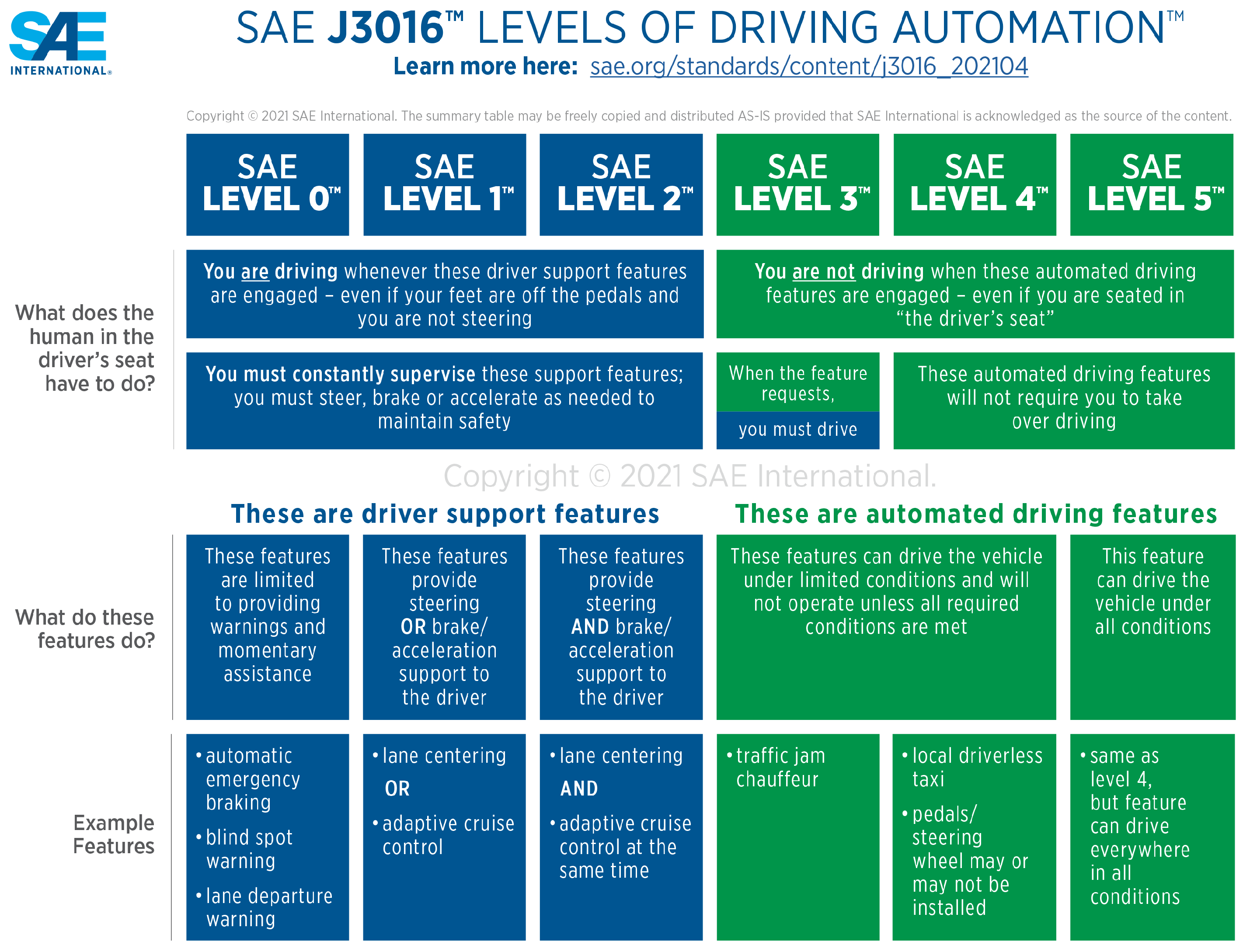
Self-driving vehicles are the next major advancement in the automotive industry. Some of the core systems that allow for autonomy in vehicles are lane-following algorithms. Lane-following algorithms are responsible for keeping the vehicle centered within the lane by using lane detection techniques to detect the pavement markings along the road. According to the SAE (Society of Automotive Engineers) International association, vehicle autonomy can be broken down into six levels, starting with SAE Level Zero all the way up to SAE Level Five (Figure 1).

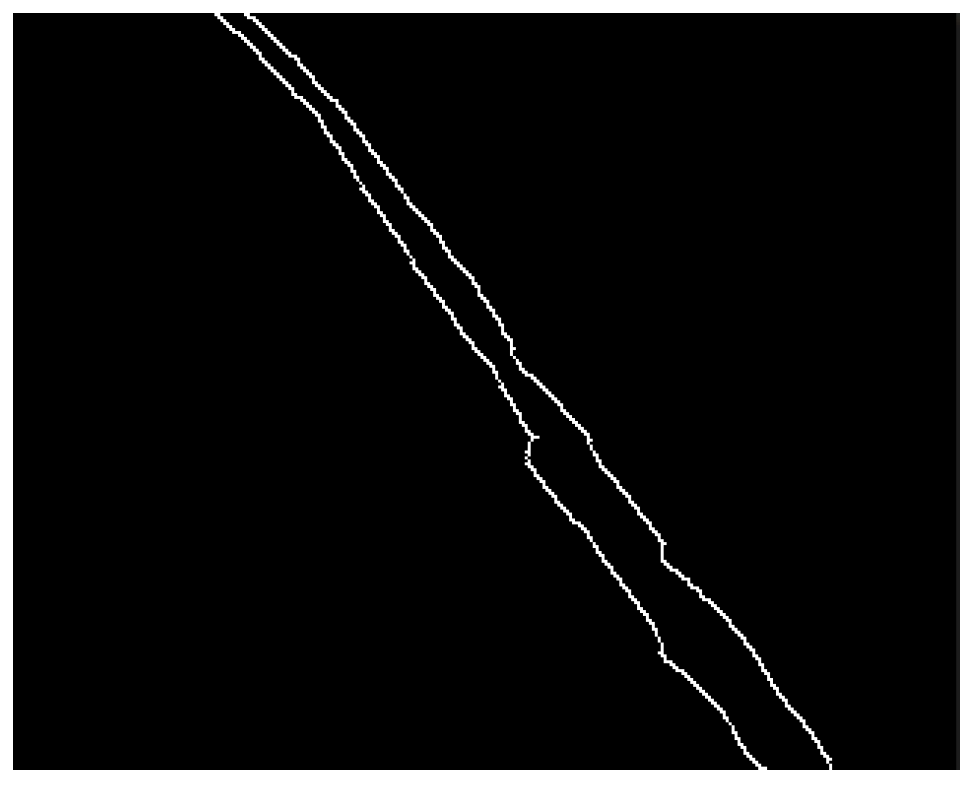
Although our algorithms are capable of steering, braking, accelerating, and lane centering, we do not target any of the SAE levels of driving automation as our algorithms forgo any kind of object detection, automatic emergency braking, and warning systems in favor of researching robust lane detection and lane centering only using computer vision. Lane detection uses computer vision to detect the lane by continuously estimating the contours of the lane markings as the vehicle is in motion, whereas lane centering uses the contours as input to monitor the position of the lane markings in relation to the position of the vehicle. As seen in Figure 1, steering assistance and lane-centering algorithms are two of the essential systems that allow for autonomy in vehicles, and since many of these systems rely on computer vision, the lane detection and lane centering problem devolves partially into a computer vision problem. Thus, this is the focus of our research.

There has been a growing recognition that theoretical results cannot capture the nuances of real-world algorithmic performance and many have started to view experimentation as providing a pathway from theory to practice [2]. In this work, we aim to experimentally analyze the strengths and weaknesses of Contour Line Detection [3], Hough Line Transform [4], and Spring Center Approximation [5] algorithms implemented in Python.

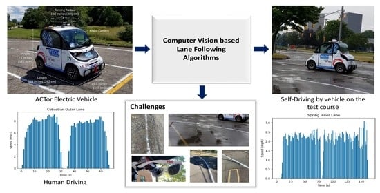
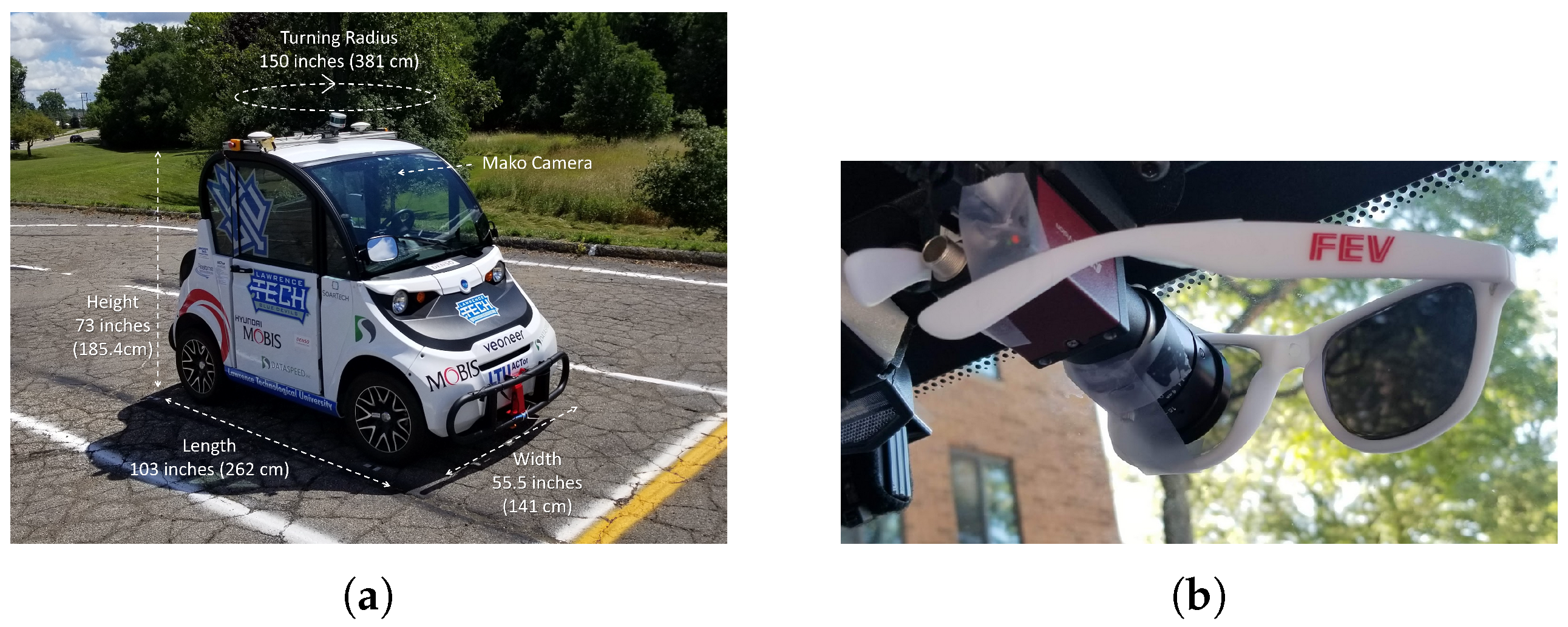
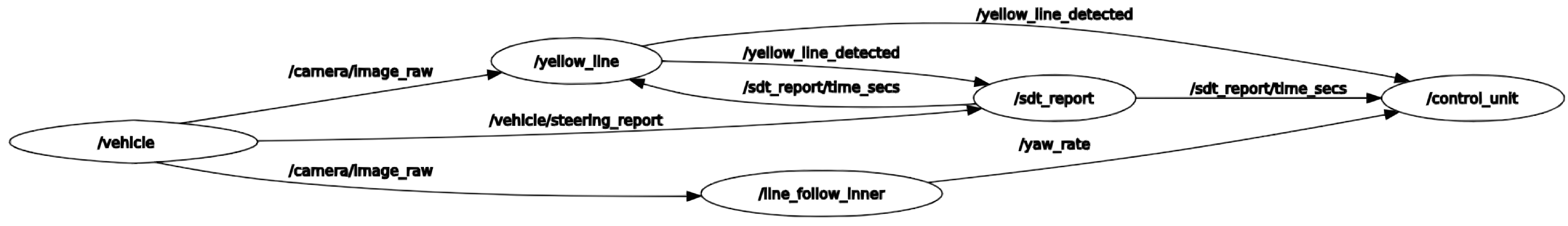
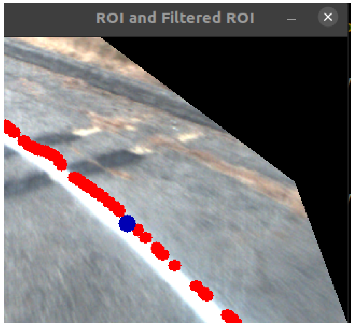
In our empirical analysis, we found that a robust lane-following algorithm must be able to deal with fading, broken-up, and missing road lane markings under varied weather conditions and be resilient to environmental obstructions, which may prevent the lane from being detected, such as shadows and reflections on the road. In this work, we tackle these challenges in the lane-following and lane-centering algorithms we developed, analyzed, and evaluated using a real street-legal electric vehicle. The key to our algorithms lies in the region of interest, filters, and yaw rate conversion function we designed. The yaw rate conversion function takes the coordinate of the centroid used by the lane-centering algorithm and converts it into yaw rates for the vehicle to use as input for steering. This allows our algorithms to work under varied weather conditions and environmental challenges. Our solutions were designed and implemented using the Robot Operating System (ROS) and OpenCV libraries in Python.

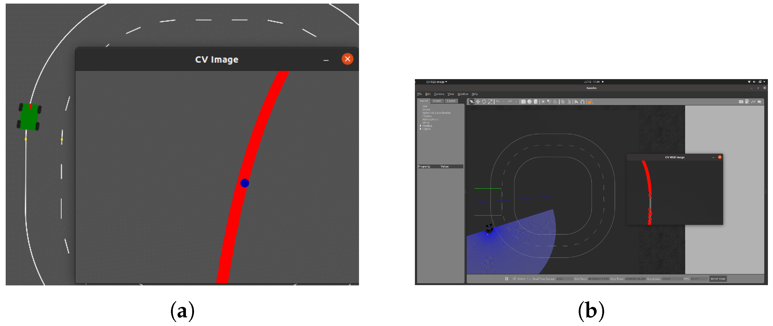
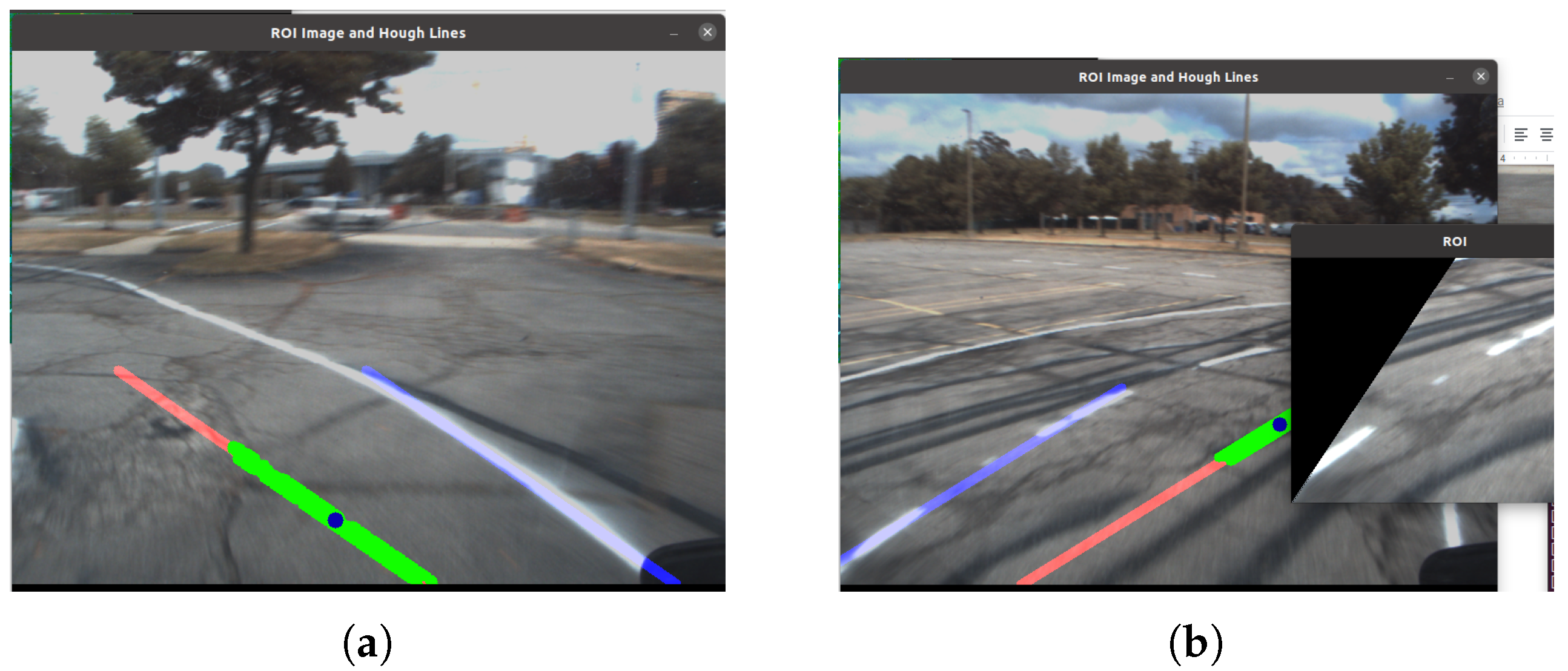
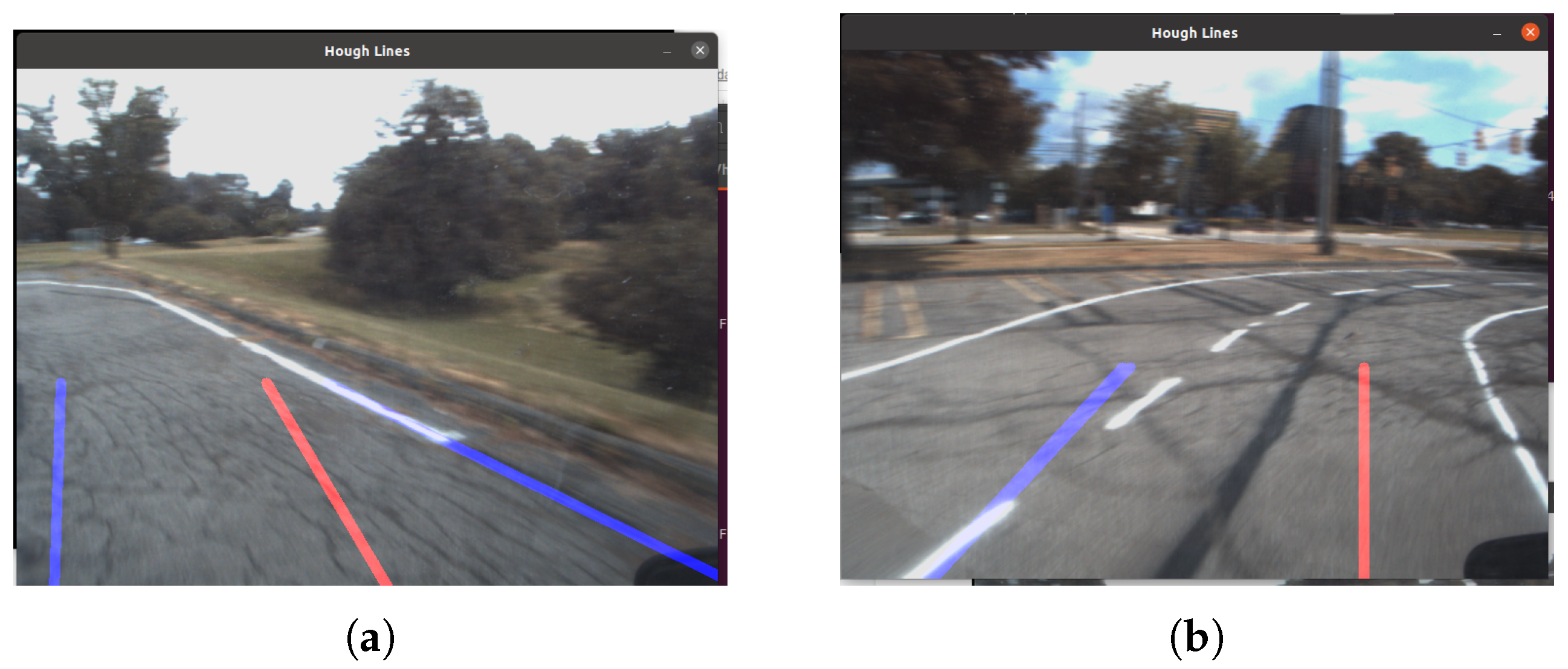
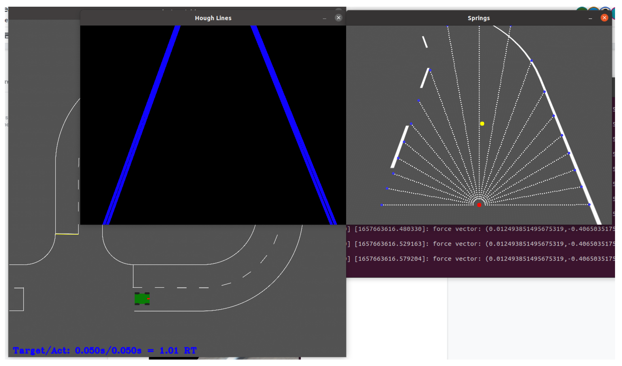
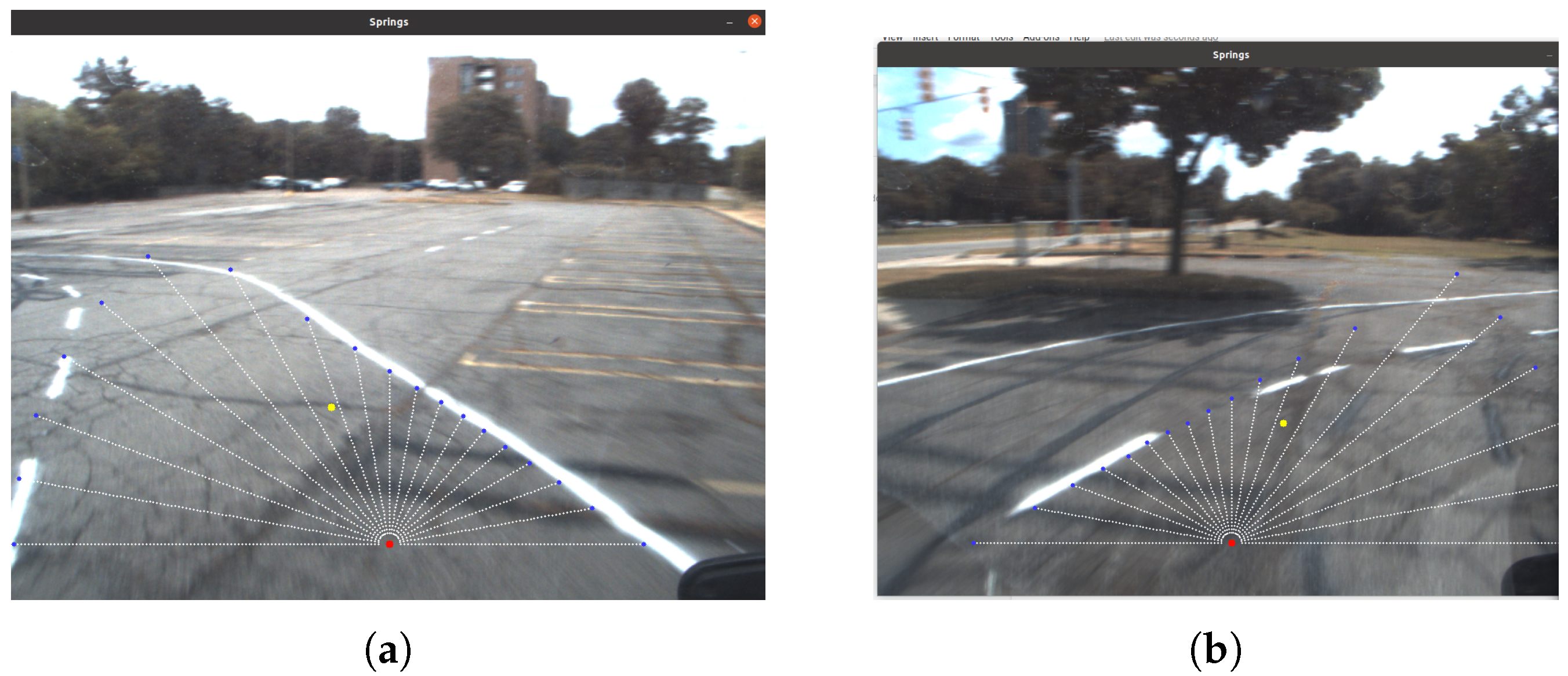
All of our algorithms work in a similar way: they lane follow by chasing a hypothetical blob that is always centered with respect to the lane. The coordinates of the blob are then converted into yaw rates, which the drive-by-wire system uses to control the steering of the vehicle. Thus, our goal is to implement this hypothetical blob that the algorithms can always rely on being in the middle of the lane. The first algorithm does this by computing the centroid of the largest contour of the edge line. This centroid is the middle point of the edge line, so we shift its position until it is in the middle of the lane relative to the edge line. The coordinates of the centroid are then converted into a yaw rate for steering. On the other hand, the second algorithm accomplishes this task by using Hough Line Transform to detect the solid white lines on both sides of the lane and then draws a hypothetical or “fictitious” line in between the white lines and computes its centroid to determine the position of the blob. The third algorithm uses Hough Line Transform to detect the road lane markings, then draws a series of rays that dynamically change in size to fit to the lane. This algorithm starts with the blob centered in the middle of the lane and uses the size of the rays to compute the forces acting on the blob to ensure it always stays in the middle of the lane using spring physics.

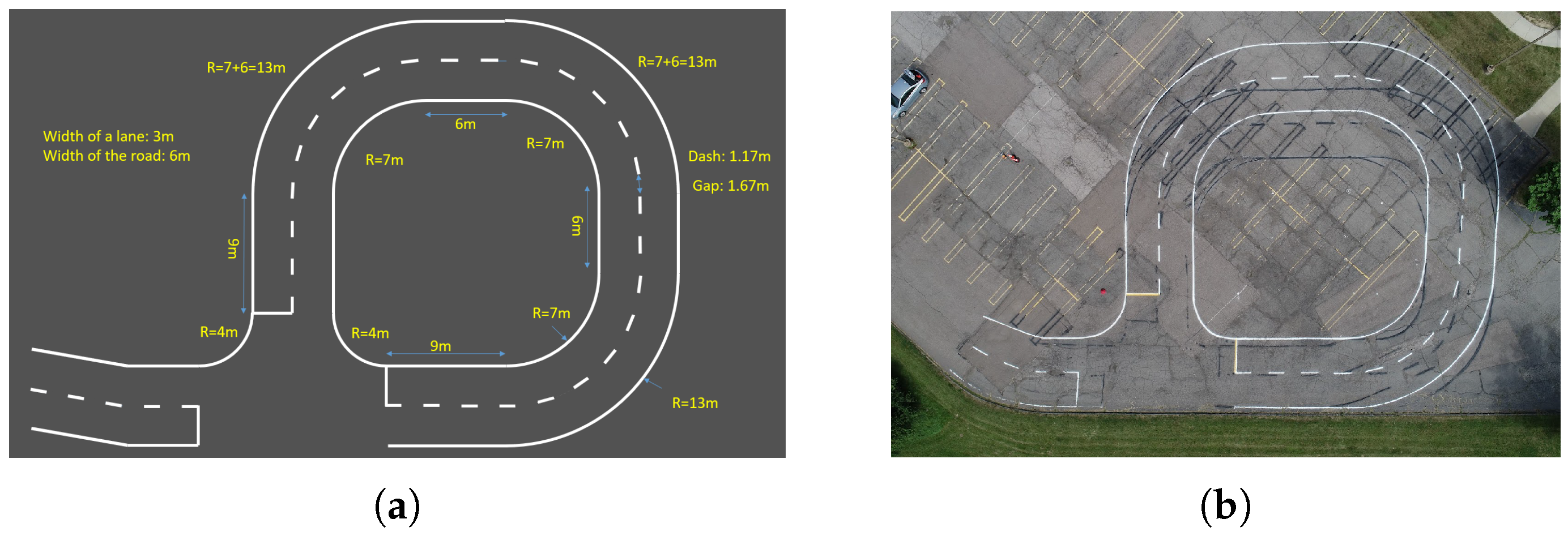
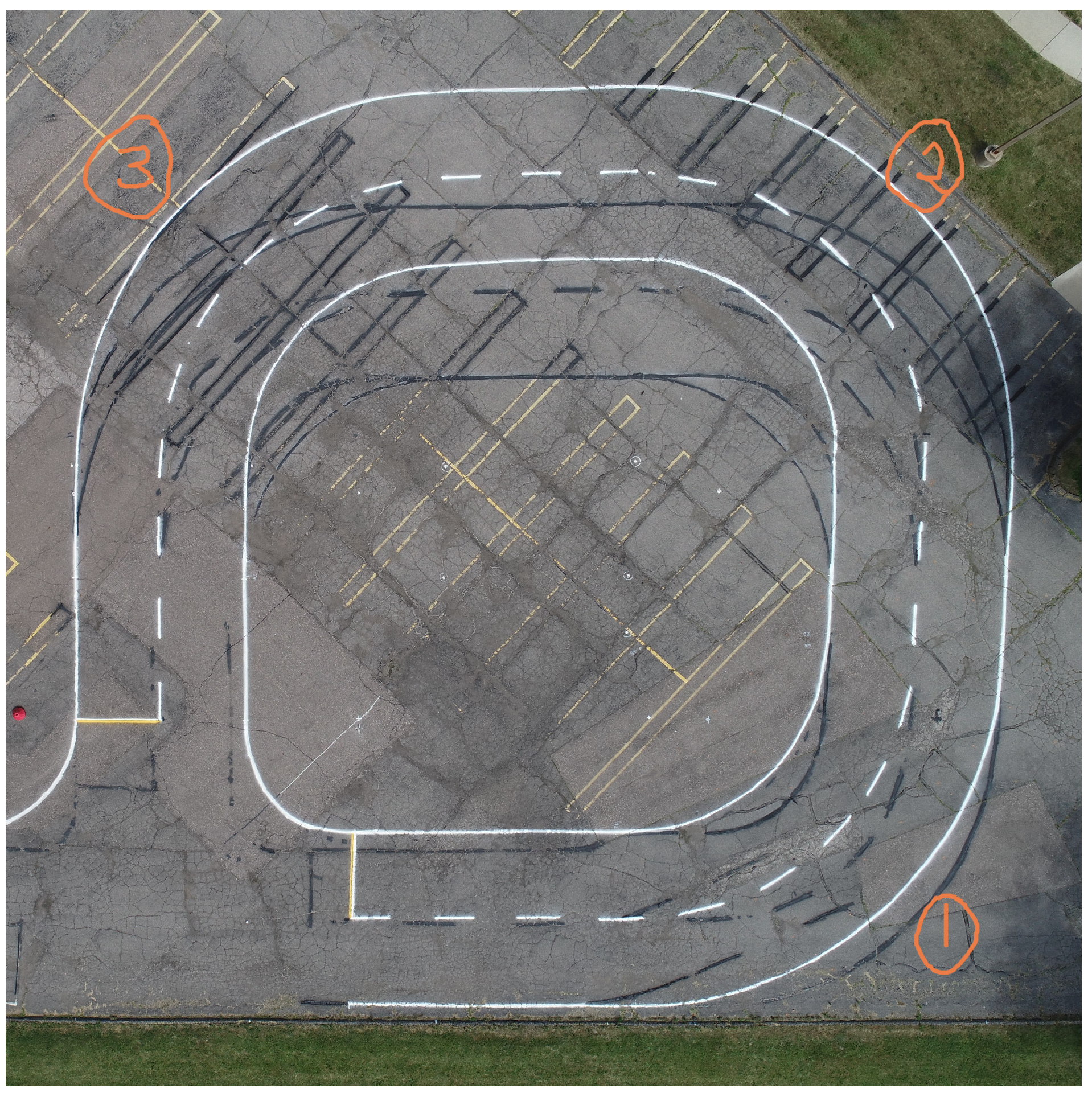
To make a fair comparison between the driving performance of the algorithms and a licensed human driver, we set a speed limit. The speed limit ensures that the algorithm can be tested safely, since the test course is circular and compact, this means that the turns are naturally sharp (see Figure 2). After testing it, we concluded that seven miles per hour is the fastest speed the algorithms can safely handle while running circles around the test course. We arrived at this value on the basis that, on average, the fastest a licensed human driver could safely complete a lap around the course was eleven miles per hour without touching the lane markings. This number is within the expectations we had considering that, in simulation, the algorithms worked consistently up to ten miles per hour given the same test course. However, even in simulation, achieving speeds higher than ten miles per hour proved difficult because of the tight turns. The driving performance of human versus algorithm are put to the test and then evaluated under the same conditions by noting advantages and disadvantages the algorithms have over the human driver and vice versa. As an example, the algorithms were better at lane-following while keeping a consistent speed than the human driver. This benchmark allows us to gauge where our algorithms stand in comparison to a human driver and to pinpoint the areas that need the most improvement to bridge the gap in performance.

Thus, the goal of this research is to develop, analyze, and evaluate self-driving lane-following and lane-centering algorithms in simulation and in reality using street-legal electric vehicles in a test course with various challenges. In our design, we intend to account for sharp curves, narrow parking lot lines, unmaintained roads, and varied weather conditions. Furthermore, we aim to compare the performance of the algorithms to each other and to a licensed human driver under a speed limit. The main contributions and novelty of this research work are summarized as follows:

• We propose multiple computer vision-based lane-following algorithms which are tested on a full scale electric vehicle in a controlled testing environment.
• The real-world testing environment has sharp curves, faded or narrow lane markings, and unmaintained roads with exposure to the weather. The algorithms have been optimized to work under these conditions. Since computer vision-based lane-following algorithms that rely on just a camera have not been evaluated under these circumstances before, our algorithms serve as a baseline for navigating unmaintained roads under varied weather conditions. Our most reliable algorithms had a success rate of at least 70% with some lane positioning infractions.
• We evaluate the driving data of the algorithms and a licensed human driver using a custom performance evaluation system, and then analyze and compare the two under a specified speed limit using reports from the vehicle’s drive-by-wire system. The algorithms are found to have a better speed control over the human driver, whereas the human driver outperformed the algorithms when driving at faster speeds while keeping to the lane.
• We test the performance of algorithms written in Python as opposed to a compiled programming language such as C++.

The remainder of this paper is organized as follows: Section 2 reviews the state-of-the-art research about lane-following algorithms for self-driving vehicles that only use a camera and computer vision. This section goes over main gaps identified in this kind of research and explains the role of our research in expanding knowledge in the discussed areas. Section 3 elaborates on the simulation, physical testing environment, and the development of the lane-following algorithms. Then, the specifics about the challenges posed by the weather and unmaintained roads are illustrated in Section 4. Section 5 discusses the results of the evaluation of the algorithms in a real-time environment on the course using a street-legal electric vehicle. The performance of the algorithms to a human driver is also compared in this section. We reiterate the main results of this work and conclude the manuscript by identifying the limitations and future avenues of work in Section 6.

2. Review of Literature

In most other research work on lane-following algorithms for self-driving vehicles using only a camera and computer vision, the algorithms are only tested in simulation. Even in simulation-based work, the lane detection is overlaid on an image or video of the road. A simulated vehicle is not used to understand the performance of lane detection algorithms at different speeds nor does it take into account the kinematics of the vehicle. Please refer to Table 1 for the summary of the literature review detailing the highlights of the papers and the research gaps identified. 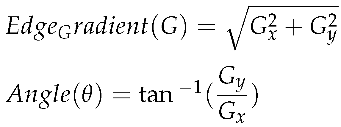In [6], the approaches in previous literature were categorized into three classes: area-based methods, edge-based methods, area-edge-combined and algorithm-combined methods. In area-based methods, the road detection problem is considered as a classification problem and regions in the image are classified into road and non-road. In edge-based methods, an edge map of the road scene is obtained, and then using a predefined geometric model matching the procedure is carried out to detect the lane. In algorithm-combined methods, several methods are carried out together in parallel to increase detection performance. According to these classifications, we use edge-based methods, and thus our prior art search covers papers in this field.

In [7], the authors test their self-driving algorithm, which involved Hough Transform with hyperbola fitting, on real-life vehicles. However, the authors mentioned that the algorithm works only on slightly curved and straight roads, and there were some problems with lane detection under certain lighting conditions. Our work aims to target these limitations by enabling the vehicle to take sharp turns within a set speed limit under different lighting conditions just using a camera and computer vision techniques.

The authors of [8,9] used several computer vision techniques for lane detection. In [8], the authors compared thresholding, warping, and pixel summation to Gaussian Blur, Canny Edge Detection, and Sliding Window Algorithm and found that the second approach was more accurate. In [9], the authors used the HLS (Hue, Light, Saturation) colorspace, perspective transform, and sliding window algorithm. We did not attempt the sliding window algorithm in this research work as the basic sliding window algorithm cannot detect dashed lines and sharp curves. We attempted different combinations of the image processing pipeline used in [8,9]; however, we observed that we gained minimal performance improvement relative to the increase in computational complexity when working on the real vehicle. We optimized the image processing pipeline for speed and efficiency by using only necessary techniques (refer Section 3 for further details) to avoid processing delays.

Table 1. Literature Review.

	Papers	Purpose	Brief Description	Research Gaps Identified
Deep Learning Approaches	[10]	Lane Detection	A spatial CNN approach was compared to sliding window algorithm. Tested in simulation.	Authors found that classical computer vision had considerably lower execution time than deep learning and no extra specialized hardware required.
	[11]	Lane Detection	LaneNet [12] was tested on a real vehicle.	Only lane centering without steering angle calculation was performed with deep learning. Moreover, due to our test course being predefined, any deep learning-based lane-centering solution would have resulted in overfitting.
	[13]	Lane Centering, and Steering Control	Transfer learning with inception network was used for lane centering and steering angle calculation. Tested on a real vehicle.	On average, the model achieved a 15.2 degree of error. This would not have worked for our course consisting of sharp turns.
Classical Computer Vision Approaches	[8,9,14,15,16]	Lane Detection	Standard Hough Line Transform, Sliding Window algorithm, Kalman Tracking, RANSAC algorithm.	These algorithms do not work well on sharp curves, varied weather conditions, nor poorly maintained roads. They also have not been tested in a real test environment.
	[17]	Lane Detection	Kalman Tracking used and RANSAC algorithm for post-processing. Tested under varied, challenging weather conditions.	The future work of the paper included explicitly fitting the curve to the lane boundary  data.
	[18]	Lane Centering and Steering Control	A nonlinear path tracking system for steering control was presented and tested in simulation.
	[7]	Lane Detection, Centering, and Steering Control	Hough Transform with hyperbola fitting. Tested on real vehicles.	Only works on slight curves, straight roads, and certain lighting conditions.
	This work	Lane Detection, Centering, and Steering Control	Blob Contour Detection, Hough Line Transform, Spring Center Approximation method. Tested on a real vehicle in a test course with tight turns, varied weather and poorly maintained road conditions.	Only tested up to 7 miles per hour. The algorithms do not meet SAE J3016 standards because they lack object detection, automatic emergency braking, and warning systems.

Table 1. Literature Review.

	Papers	Purpose	Brief Description	Research Gaps Identified
Deep Learning Approaches	[10]	Lane Detection	A spatial CNN approach was compared to sliding window algorithm. Tested in simulation.	Authors found that classical computer vision had considerably lower execution time than deep learning and no extra specialized hardware required.
	[11]	Lane Detection	LaneNet [12] was tested on a real vehicle.	Only lane centering without steering angle calculation was performed with deep learning. Moreover, due to our test course being predefined, any deep learning-based lane-centering solution would have resulted in overfitting.
	[13]	Lane Centering, and Steering Control	Transfer learning with inception network was used for lane centering and steering angle calculation. Tested on a real vehicle.	On average, the model achieved a 15.2 degree of error. This would not have worked for our course consisting of sharp turns.
Classical Computer Vision Approaches	[8,9,14,15,16]	Lane Detection	Standard Hough Line Transform, Sliding Window algorithm, Kalman Tracking, RANSAC algorithm.	These algorithms do not work well on sharp curves, varied weather conditions, nor poorly maintained roads. They also have not been tested in a real test environment.
	[17]	Lane Detection	Kalman Tracking used and RANSAC algorithm for post-processing. Tested under varied, challenging weather conditions.	The future work of the paper included explicitly fitting the curve to the lane boundary  data.
	[18]	Lane Centering and Steering Control	A nonlinear path tracking system for steering control was presented and tested in simulation.
	[7]	Lane Detection, Centering, and Steering Control	Hough Transform with hyperbola fitting. Tested on real vehicles.	Only works on slight curves, straight roads, and certain lighting conditions.
	This work	Lane Detection, Centering, and Steering Control	Blob Contour Detection, Hough Line Transform, Spring Center Approximation method. Tested on a real vehicle in a test course with tight turns, varied weather and poorly maintained road conditions.	Only tested up to 7 miles per hour. The algorithms do not meet SAE J3016 standards because they lack object detection, automatic emergency braking, and warning systems.

In [15], the authors propose steerable filters for combating problems due to lighting changes, road marking variation, and shadows. These filters seem very useful for combating the shadow problem and especially for tuning to a specific lane angle. For lane tracking, in this paper, the authors opt for using a discrete time Kalman Filter. We did not go for this approach in our work as the Kalman filter provides a recursive solution of the least square method, and it is incapable of detecting and rejecting outliers which sometimes leads to poor lane tracking as stated in [6]. In [14], two different approaches were taken based on whether the road was curved or straight. For a straight road, the lane was detected with Standard Hough Transform. For curved roads, complete perspective transform followed by lane detection by scanning the rows in the top-view image was implemented. As an improvement to this, the authors in [19] adopt a generalized curve model that can fit both straight and curved lines using an improved RANSAC (Random Sample Consensus) algorithm that uses the least squares technique to estimate lane model parameters based on feature extraction.

In [10], the authors propose a computer vision algorithm called HistWind for lane detection. This algorithm involves filtering and ROI (region of interest) cropping, followed by histogram peak identification, then sliding window algorithm. HistWind is then compared with a Spatial CNN (Convolutional Neural Network) and the results are comparable for both, although HistWind has a considerably lower execution time. In [13], the ACTor (Autonomous Campus TranspORt) vehicle was used for testing a deep learning-based approach for lane centering using a pretrained inception network and transfer learning. However, since this approach is computationally intensive and requires specialized hardware, we did not attempt deep learning-based solutions in our work. Additionally, due to the test course being predefined, any deep learning-based solution would have resulted in an overfitted model. The computer vision-based approach was chosen for this work because it is usually simpler and faster than any other technique that requires specialized hardware.

From the above papers, we have identified that the improved RANSAC algorithm [19], Kalman Tracking [19], sliding window algorithm [19], and spline models such as [20] detect and trace the exact curvature of the boundary of road. Out of these, as elaborated above, the RANSAC algorithm seems promising as seen in [17]. Taking the characteristics of the various lane models and the needs of lane detection in a harsh, real-time environment into consideration, we propose fast and efficient lane keeping algorithms which use Contour Detection (which traces the exact curvature of the road) and Hough Line Transform (which linearly approximates the curvature of the road).

3. Materials and Methods

3.1. Simulation

We use the Robot Operating System (ROS) and Python for the development of our algorithms. We test the code on two simulators: simple-sim [21], which is a 2D simulator, and Gazebo, which is a 3D simulator. We use the OpenCV library for implementing the computer vision algorithms.

3.2. Real World

3.2.1. Environment

The test course is in Parking Lot H located at Lawrence Technological University in Southfield, Michigan, USA. It is a two-lane course, with an intersection at the bottom left where the vehicle is programmed to stop at the yellow line before crossing it using a dead reckoning turn. The challenge for each of the algorithms is to make two laps around the course in succession for both the inner and outer lanes. The vehicle is meant to start with the front wheels behind the yellow line, then proceed to make the dead reckoning turn, and continue to drive until it has to make a stop for three seconds at the starting point and repeat. The test course is out in the open affected by the weather; it has potholes, sharp curves, fading and narrow road lane markings, and yellow parking lot markings as seen in Figure 2.

3.2.2. Vehicle Specifications

ACTor (Autonomous Campus TranspORt) is built on top of a modified Polaris Gem e2 (Figure 3) provided by a joint sponsorship from two companies: Mobis and Dataspeed. Mobis provided the base vehicle, and Dataspeed installed the drive-by-wire system. Lawrence Technological University, DENSO, Dataspeed, Veoneer, SoarTech, and Realtime Technologies provided Dataspeed’s drive-by-wire system, vision sensors, 2D and 3D LIDARs (Light Detection and Ranging), GPS (Global Positioning System), on-board computers, and all other hardware. The Polaris Gem e2 (Polaris, Medina, MN, USA) has a top speed of twenty miles per hour, and a range of approximately twenty miles. For this research project, we limit the speed to seven miles per hour for safety reasons since the algorithms are tested under the supervision of humans on board.

We use a Mako G-319 Camera (Allied Vision, Exton, PA, USA) for lane-following. The Mako camera has a resolution of 2064 × 1544 pixels with a max frame rate of 37 frames per second at max resolution, and it has native ROS support.

3.3. Code Architecture

All of the lane-following algorithms follow the same architecture for the sake of simplicity and modularity. We have four nodes: the SDT (Speed, Distance, Time) report, yellow line, line follow and the control unit as seen in Figure 4. The SDT report publishes the data required for evaluating the algorithms. The yellow line node is responsible for detecting the yellow line by counting the number of yellow pixels for a specified number of frames in a custom region of interest. The line follow node is responsible for converting the coordinates of the center blob into yaw rates used for steering by the drive-by-wire system. The control unit is responsible for connecting the algorithm to the drive-by-wire system to pass the computed yaw rates and the speed values input by the user. Further details of the mathematics behind each of these nodes is provided below.

The filters applied are also consistent across the algorithms and a region of interest is customized for each algorithm.

3.3.1. SDT Report Node

The Speed, Distance and Time (SDT) report is a node that keeps track of the instantaneous speed, the distance traveled, and the time while the vehicle is in motion and makes this information available to other nodes. The instantaneous speed comes from the steering report published by Dataspeed’s drive-by-wire system installed on the vehicle. This node keeps track of the time elapsed by using the time module from the ROS client library for Python while the vehicle is in motion. Finally, given the instantaneous speed and the time, we computed the distance traveled by approximating it using the Riemann sum using the equation below.

$$distance=\sum _{i=n-1}^n(speed\ast \Delta time)$$

3.3.2. Yellow Line Node

The yellow line node detects the yellow line on the course by using a 351 × 160 region of interest and converting it to the HLS colorspace. Using the converted image, this node uses OpenCV’s inRange and findContours functions to obtain a binary image with only the yellow pixels within an HSL range and computes the area of the largest contour as seen in Figure 5. The algorithm determines whether or not what it sees is a yellow line by checking for an area greater than six-hundred pixels for seven consecutive frames while the vehicle is in motion.

Once the yellow line is detected, it publishes a Boolean message which the control unit then listens for to slow down the vehicle for a few seconds until it comes to a full stop at the yellow line for three seconds, and then performs the dead reckoning turn depending on whether it is in the inner or outer lane. The dead reckoning proved to be more reliable at the intersection, as there are no road lane markings to follow during the duration of the turn. This algorithm can be improved further by combining this method with Hough Lines Transform to look for lines of a specific slope instead of solely relying on color detection.

3.3.3. Line Follow Node

The line follow node is the only node which varies by algorithm. It is solely responsible for computing the yaw rate in radians per seconds and publishing it to the control unit.

3.3.4. Control Unit Node

The control unit subscribes to the three nodes described above and links them to the drive-by-wire system. The yaw rates computed in the line follow node and the speed values input by the user are published as a command to the vehicle through this node. This node also publishes control messages to the drive-by-wire system during the dead reckoning turn (the turn at the intersection). In order to know when to switch from lane-following to dead reckoning, and vice-versa, the control unit subscribes to messages sent by the yellow line node. The dead reckoning parameters are sensitive to weather conditions. This is because the sunlight present at the time affects how fast the seven consecutive frames of yellow were detected, thus resulting in stopping early before the yellow line or stopping late past the yellow line.

3.3.5. Filters

We apply a white balance filter as in ([22]) that converts the RGB (Red, Green, Blue) image to the CIELAB (L* for perceptual lightness, and a* and b* for the four unique colors of human vision: red, green, blue, and yellow) (or L*A*B) colorspace as it approximates human vision. This provides a lightness component and two color components. The white balance filter adjusts the image such that the colors in the image are naturally seen without being affected by the color of the light source. The filter compensates for the color hue of the light source. In the case of direct sunlight, we apply this white balance filter twice to enhance the algorithm’s ability to detect the lane under sunlight.

Additionally, since algorithms are sensitive to the weather conditions, we implement the ability to dynamically adjust the parameters of the filters at the time of testing. This method uses the HLS (Hue, Light, Saturation) colorspace to create a mask for detecting the white lane markings. The HLS colorspace simplifies the process because only the L value needs adjusting depending on the weather. The mask is created by converting the images from the camera to grayscale and then smoothing them using a 2D convolution kernel ([23]). HSL masking was also useful as it allows only white and yellow regions to pass through into a grayscale image. Lastly, we pass the smoothed grayscale images to the Canny Edge Detection function to obtain the best results for detecting the white lane markings. The math behind these functions is shown in Figure 6.

The Canny Edge Detection function [24] is able detect the edges of objects in the images by comparing the gradient magnitude of a pixel to the pixels on its sides. If the magnitude is larger than the adjacent pixels in the direction of maximum intensity, the Canny Edge Detector classifies that pixel as an edge as shown in Figure 7. This function also uses non-maximum suppression and thresholding. This technique is used to extract the morphological information from the images and to reduce the amount of data that is processed. Figure 8 depicts the image after the application of all of the filters.

3.3.6. Region of Interest

Seeing as the raw camera footage contains substantial noise and extraneous information, we decided to implement a region of interest to target only the region needed to detect the road lane markings. This is accomplished by using a numpy array of size five, which corresponds to the number of sides in the polygon-shaped region we mapped out using the fillPoly function in the OpenCV library. The end result is a region of interest tailored to the needs of each algorithm for detecting the lane markings. We also had the idea of implementing a dynamic region of interest using a numpy of size eight that would automatically change its shape based on the coordinates of the centroid. This further cropped the image, however, it would sometimes leave in extraneous information that interfered with the algorithms. Future experimentation with the array size and parameters could lead to better results.

As can be seen in Figure 9, the image after applying a region of interest is cleaner and eliminates noisy data such as extraneous lines on the road and on the horizon. This allows our algorithm to focus on the actual lane markings rather than attempting to draw a contour or Hough lines on something such as grass, yellow parking lot markings, or any additional irregularities on the course that our filters are not able to detect.

3.4. Algorithm I (Blob)

Contour Line Detection, Offset Lane Centering, and Proportional Control Yaw Rate Calculation using Contour

The goal of all lane-following algorithms is to identify the center of the lane and to steer the vehicle towards it [3]. The first algorithm is the simplest of the three implemented. The algorithm was implemented using the filtered image as input.

In this algorithm, the key to getting the vehicle to follow the white line smoothly consisted of two steps:

• Compute the centroid of the largest contour using the OpenCV library;
• Devise a formula to convert the coordinates of the centroid into yaw rates (in radians per seconds).

We drew a circle at the centroid of the largest contour, which presents the center of the white line in the camera’s view. The vehicle was commanded to try to keep that circle in the same area in the image while in motion.

We refined this algorithm in simulation by computing the difference between the x value of the contour’s centroid and subtracting it from the y value of the vehicle’s camera centroid. Then, dividing that by a correction value, which we obtained by multiplying a constant by the x value of the vehicle’s camera centroid. This yields a yaw rate that is proportional to the difference between the x position of the contour’s centroid and the centroid of the vehicle’s camera view.

For lane centering, only one of the lane lines was detected and the vehicle was centered to maintain a certain distance from the detected line. The simulated vehicle was able to follow the lane at a high speed of 16 mph with no discernable jitter.

Figure 10 and Figure 11 show the working of the blob detection algorithm in the simulator and the real-time environment respectively.

3.5. Algorithm II (Hough)

Probabilistic Hough Transform Line Detection, Fictitious Center Lane Line Using Offset for Lane Centering, and Proportional Control Yaw Rate Calculation using Contour

Hough lines have been used in previous lane keeping algorithms, including those used by real vehicles [7]. We implemented the Probabilistic Hough Line Transform function [4] to the filtered image for line detection. The standard Hough Transform is used to determine the parameters of features such as lines and curves within an image. In the case of line detection, a single edge pixel is mapped to a sinusoid in 2D parameter space representing all possible lines that could pass through that image point. This point-to-curve transformation is the Hough transformation for straight lines. When viewed in Hough parameter space, points which are collinear in the cartesian image space become readily apparent as they yield curves which intersect at a common point. Probabilistic Hough Transform is an optimization of the Hough Transform. It does not take all the points of the line into consideration. Instead, it takes only a random subset of points which is sufficient for line detection. The Probabilistic Hough Lines are found using the parametric form for a standard line equation:

$$\rho =xcos\theta +ysin\theta$$

The methods we utilize after the implementation of the Probabilistic Hough Line Transform deviates from prior research. The slope of each line is calculated and all lines with a positive slope are averaged to come up with the left line and all lines with a negative slope are averaged to come up with the right line.

For lane centering, we used two different methods:

• We offset the right line in case of outer lane-following and the middle line in case of inner lane-following according to the range of view of the camera.
• We averaged the left and right slopes to obtain a middle line.

For the yaw rate calculation, we used two different methods:

• We used the contour detection line-following method on the center line. (Refer Section 3.4)
• We used an equation that we came up with which directly uses the middle line to convert the point furthest away from the screen to a yaw rate.

For yaw rate calculation directly with the x coordinate from the center line, we used the center error (refer Figure 12) and divided it by a large gain value to obtain a small yaw rate.

We tested combinations of the above lane centering and yaw rate calculation methods to arrive at four variations of the same algorithm. The case wherein we used offset lane centering and contour detection on the center line worked the best in both simulation and real life tests. Thus, this was chosen as the implementation for algorithm II. This algorithm is novel as it is a combination of Algorithm 1 (refer Section 3.4) and the Hough Transform. Figure 13, Figure 14 and Figure 15 show the working of the Hough algorithm in the simulator and the real-time environment. Figure 16 and Figure 17 depict the different ROIs used for the different variations of the algorithm.

3.6. Algorithm III (Spring)

Hough Transform Line Detection with Spring Method Center Approximation for Lane Centering

Hough line detection is applied to find all the lines in the filtered image. All the 45° lane lines are extended to form an X to account for cases where there are broken or dashed lines in order to enable the automobile to follow a continuous path. The spring method center approximation method [5,25] is then used on these lines. This algorithm’s objective is to use spring physics as a dynamic control model to move the vehicle’s center (VC) to the lane’s center (LC). This works because the x component of the spring’s push force is in equilibrium when the car is in the middle of the lane.

To transfer the force into steering input, the rays that intersect with the line mask are detected once they have been generated from the VC point. The force may be represented as a push or pull force on the point LC using the ray lengths. The last step involves calculating the steering input using the horizontal component of the force to move the car right or left and center it in the lane. We adapted and optimized this algorithm to work in Python and fit in our code architecture.

Figure 18 and Figure 19 show the working of the Spring algorithm in the simulator and the real-time environment. Figure 20 depicts the ROI used in the real-time environment.

Table 2. Summary of the algorithms implemented.

	Line Detection	Lane Centering	Proportional Yaw Rate Control	In Simulation	In Real-Time Environment
Algorithm 1	Contour	Offset	Using the x coordinate from the centroid	Worked well. No jitter even at high speeds.	Works. This is the algorithm being used for demonstration. Jitter present in real life even at low speeds.
Algorithm 2	Probabilistic Hough Lines, then Contour	Average Center Lane Line	Using the x coordinate from the from centroid	Worked, but jitter present even at low speeds.	Could not do the sharp turns, lane departures present.
	Probabilistic Hough Lines	Average Center Lane Line	Using the x coordinate from the average center lane line	Worked better than above in simulation. Slight jitter even at low speeds.	Could not do the sharp turns, lane departures present.
	Probabilistic Hough Lines	Offset	Using the x coordinate from the offset center lane line	Worked well. Jitter present at high speeds.	Works, but requires future adjustment to find a perfect equation to calculate the proportional yaw rate.
	Probabilistic Hough Lines, then Contour	Offset	Using the x coordinate from the centroid	Worked well. Jitter present at high speeds.	Works. Algorithm being used for demonstration. Fastest and smoothest algorithm. Jitter present in real life only at higher speeds.
Algorithm 3	Hough Lines	Spring Force	Using the mean force value	Worked well. Jitter and lane departures present at medium to high speeds.	Works. This is the algorithm being used for demonstration.

summarizes the design and performance considerations of the three main algorithms implemented and includes the four variations of the Hough algorithm tested.

4. Challenges

This research study is novel because we tested our algorithms under challenging situations including dynamic lighting, varied road conditions, and distractions that would confuse our camera and interfere with our algorithms. We had to plan for and overcome all of these obstacles since people travel at various hours of the day and on unreliable roads.

4.1. Environment Challenges

Lawrence Technological University’s Lot H Course has many inconsistencies in its lane lines as the course is meant to represent the imperfections of real-world road conditions. Large portions of the lanes have potholes, cracks, and bumps, which interferes with the vehicle’s speed control, as well as the algorithms’ ability to detect the lane. Moreover, since the test course replicates an unmaintained road, the lane lines are narrower and the markings are more faded than many real-world roads, and hence harder to detect with our algorithms. As a result of this and the weather, our lane detection function would sometimes lose track of the lane causing the vehicle to drive off the road. For this reason, we decided to implement a shadow creep functionality to prevent this behavior. Our shadow creep implementation creates an artificial middle lane line for when the Hough lines are lost until the lane detection algorithm recovers. However, this method was was unsuccessful so instead we secured a strip of white reflective tape along the segments of the lane that were faded or missing as seen in Figure 21.

In Figure 22a, we see that there are instances where there are yellow parking lines that are close to the white lane lines. This creates the issue of premature yellow detection, resulting in the ACTor stopping and turning before reaching the stopping area. The solution that we came up with was to design and implement a region of interest tailored specifically for detecting the yellow line as seen Section 3.3.6.

As shown in Figure 22b, shadows from nearby trees and objects obscure the lane and breaks the lane detection algorithm due to the drastic change in brightness. This paired with our restriction of only being able to use the single Mako G-319 Camera for lane-following created a problem. To fix this problem, we implemented a dynamic reconfiguration menu and added an option to adjust the L (or light) value in the HLS colorspace we use in our filters for detecting the lane. When the shadow obscures the lane, the brightness drastically drops, which means all we needed to do was find a way to increase the brightness of the live camera footage when it happens. By adding an option to dynamically change the L value, we were able to solve the problem.

Since the camera was installed behind the windshield, our algorithms struggled in sunny conditions due to overexposure. Our stopgap solution was to tape a tinted sunglasses lens to the camera to polarize some of the light, but many times this did not suffice and our algorithms could not work properly as we relied on the camera to guide us through the course. Additionally, when it rained, the oil mixed in soil created reflective puddles on the ground, and the raindrops on the windshield increased the level of noise in the camera footage as shown in Figure 23. This made it more difficult for our algorithms to recognize the lane lines as the puddles were reflecting the white clouds overhead. The camera was also installed in a location out of the wipers reach, so it could not wipe off the raindrops off the windshield. However, the region of interest and filtering techniques implemented were robust and the algorithms were unaffected by rainy conditions (please refer to Appendix A). However, the filtering can still be improved and is an area for future quantitative study [26].

4.2. Code and Simulation Challenges

Though simulators have in the past been used to successfully transfer learning from one domain to another without retraining, including in self driving [27], in this case, the code that worked well in simulation but struggled in reality, as the simulation failed to account for the nuance and complexity of the real-world environment. The algorithms’ movement in the simulated environment was not smooth or uniform at higher speeds. In real life, most of the algorithms had poor steering control leading to unsteady movements of the vehicle when testing due to the conditions of the unmaintained road.

We tested perspective transform and Bird’s Eye View transform but found that these transformation techniques were ineffective for our uses. We also tried median blur, histogram equalization, dilation, Laplacian, Gaussian, and Sobel filters. However, we found these operations added little performance improvements relative to their computational complexity. In consideration of speed, we applied only the most necessary filters so that our algorithms could work well.

All nodes in ROS run in parallel so ROS was chosen for development purposes to be able to make use of the available computational resources on the vehicle. However, we still observed that there were delays in the processing speed as sometimes the masked image would not change despite the vehicle being in motion. This is an area that would benefit from increased computational power and could possibly increase the speed and performance of the vehicle and algorithms. It is also worth mentioning that this could be one of the limitations of implementing our algorithms in Python.

5. Results

An evaluation program was used to collect the total time, average speed, and speed infractions of a successful run for each method. An external evaluator recorded the number of times the vehicle would either touch a lane line or drift outside the lane. One of the Teaching Assistants was arbitrarily chosen as the evaluator and assigned to follow the vehicle across the test course. Markings were made on a paper version of the track where the vehicle touched a line, departed from the lane, or for the dead reckoning turn error. In addition, the weather conditions at the time and any additional comments were also noted. Since the same person evaluated all of the algorithms, the key was uniform and left up to the evaluator’s discretion. In addition, rosbags were recorded using the vehicle’s drive-by-wire system to corroborate and verify the evaluator’s sheets.

A run is defined as a failure if the human driver has to manually use the brake to stop the vehicle from hitting the curb or going off the predetermined course. In case of a lane departure wherein the algorithm is unable to follow the lane anymore, this case would also be considered a failure. In the dead reckoning turn, if the vehicle turns too much to the right in the case of the inner or outer lane turn, it is a failure case. If it turns too much to the right in the case of the outer lane-following, it hits the curb. If it turns too much to the right in the case of inner lane-following, the algorithm loses the middle dashed line or the outer line too according to the region of interest used. In both of these cases, it results in a failure case as the algorithm is unable to proceed following the lane.

Table 3. Summary of Results Data.

	Inner/Outer	Success Rate (%)	Time Taken to Complete 2 Laps (s)	Best Average Speed for Both Laps (mph)	Distance Covered above or below Speed Limit (m)	No. of Line Touches
Algorithm 1—Blob	Outer	66.67	193.02	1.999	3.352	0
	Inner	50	153.22	2.108	4.962	3 in lap 1, 4 in lap 2
Algorithm 2—Hough	Outer	77.78	86.88	4.476	8.142	0
	Inner	66.67	163.41	2.088	4.768	0
Algorithm 3—Spring	Outer	33.33	163.68	2.147	2.77	infinite 1
	Inner	75	154.02	2.13	3.364	0
Best Human Driver	Outer	100	75.00	5.854	71.03	0
	Inner	100	71.14	5.185	2.292	0

¹ The vehicle’s wheels were on the line throughout most of the lap (but it did not depart the lane).

below shows the recorded data for the official runs of the algorithm. Each run, whether it was successful or not, was recorded as a rosbag file for future analysis. An external evaluator was responsible for noting the results. Refer to Appendix A for the details of each of the official runs. The total number of recorded runs for each algorithm was used to determine the average success rate.

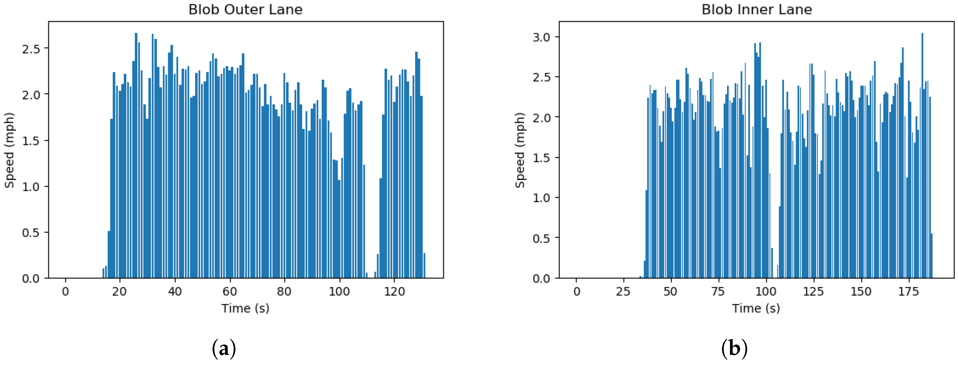
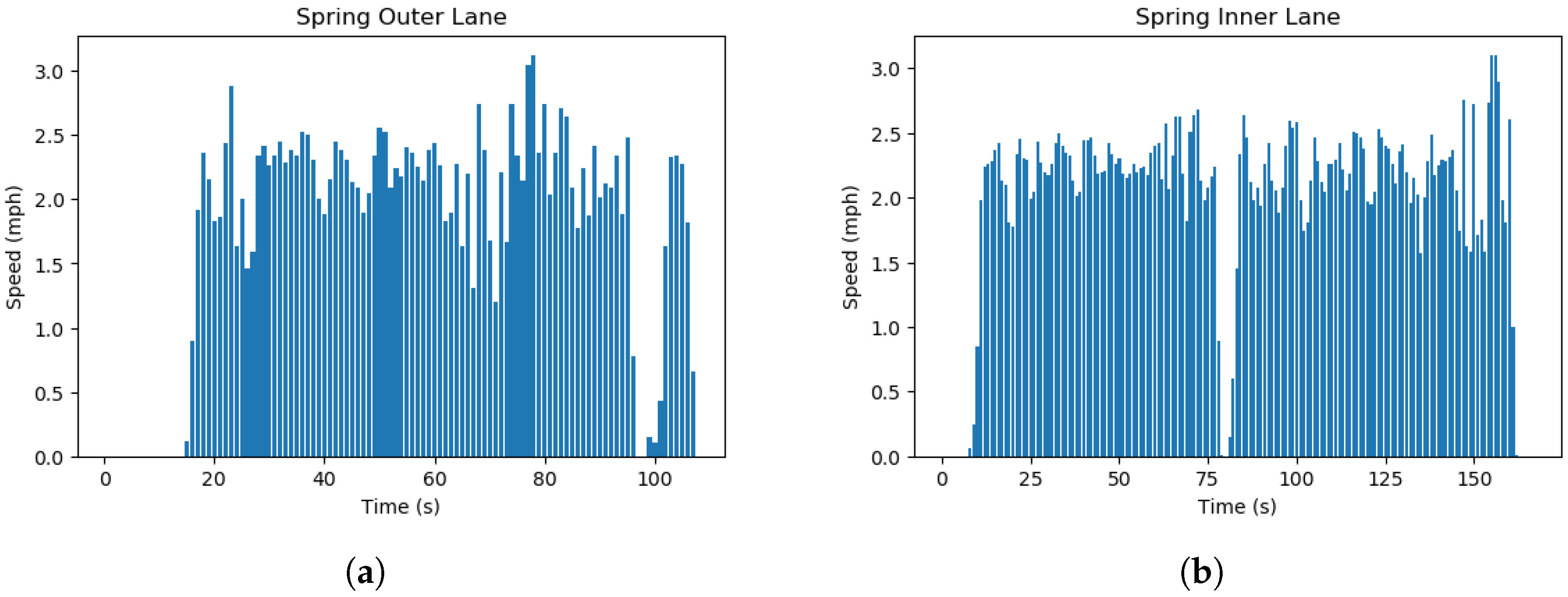
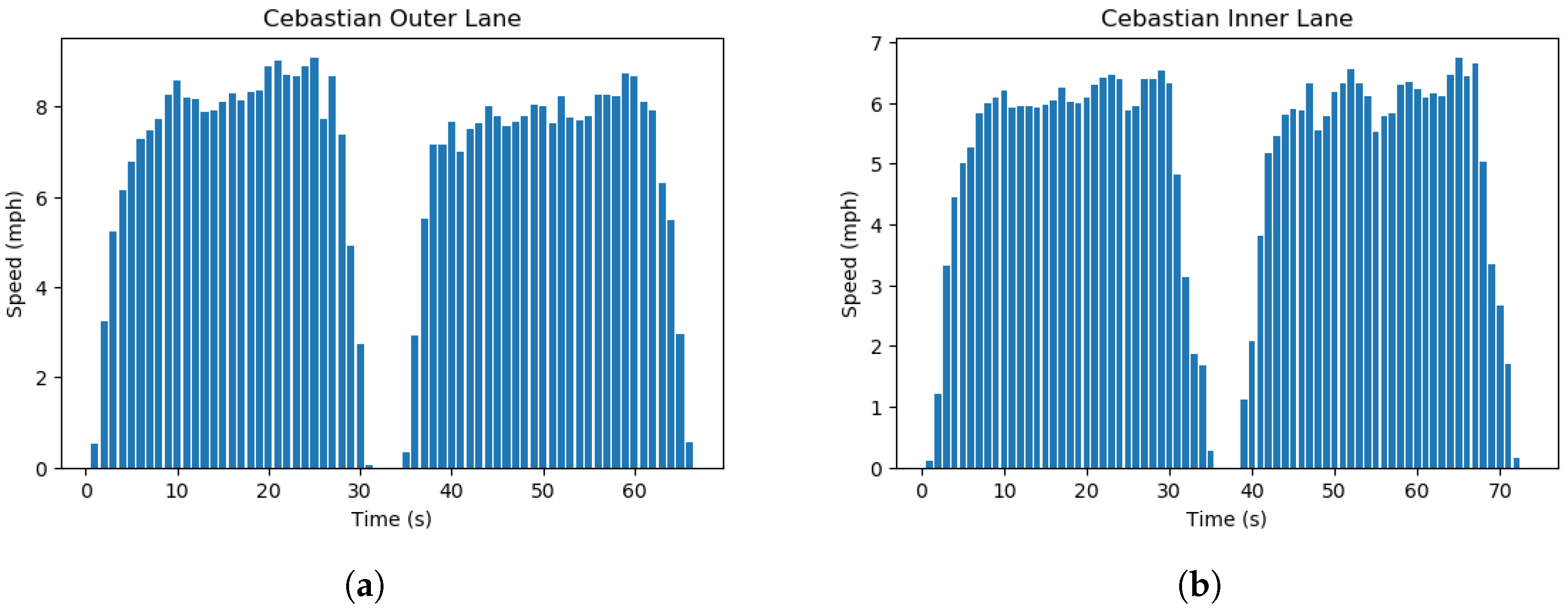
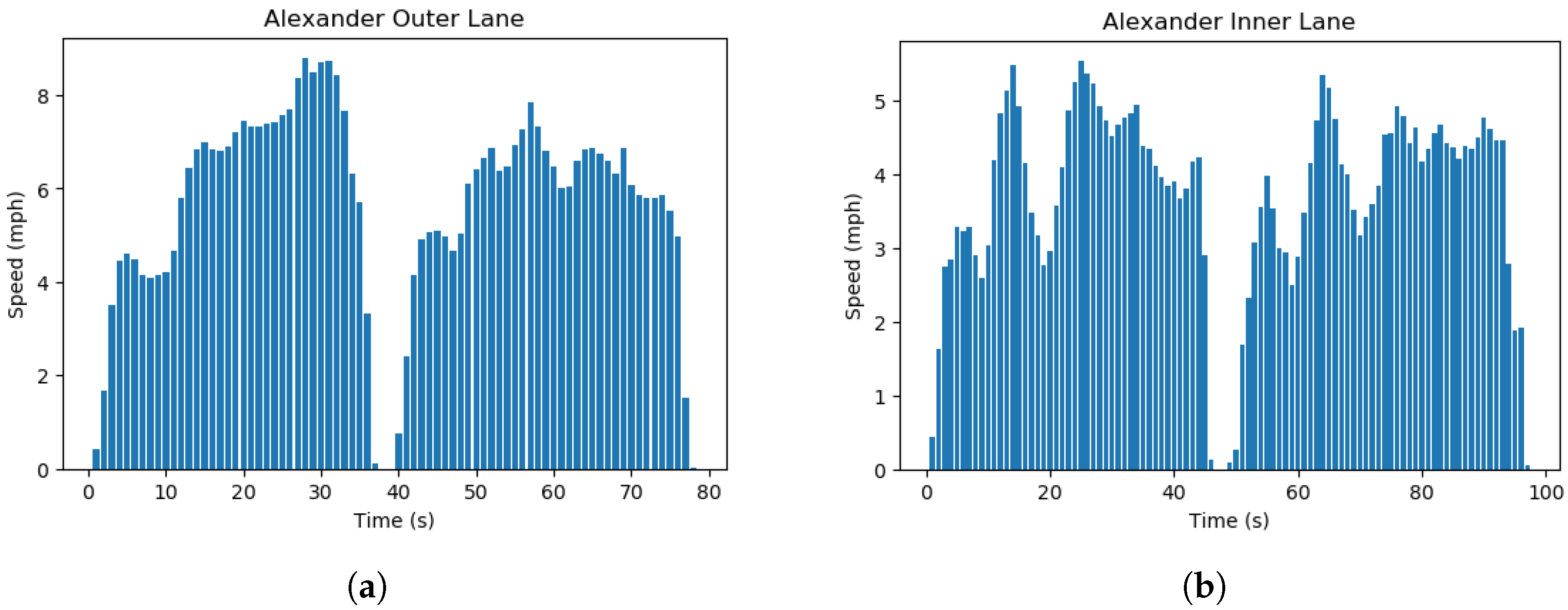
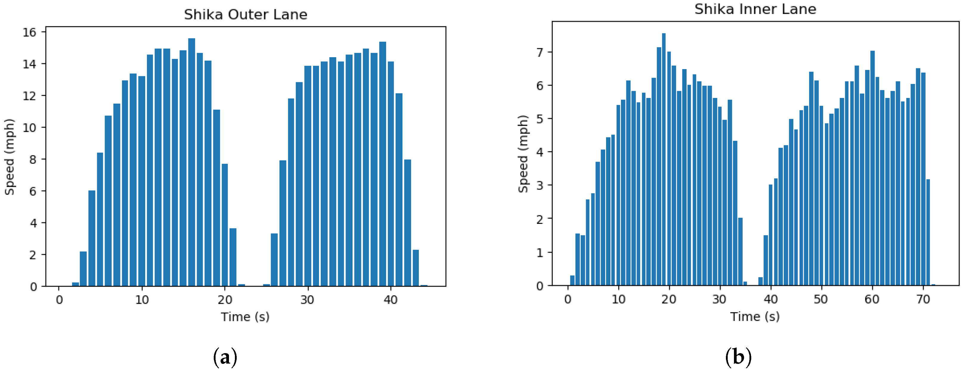
The official runs of each algorithm on the inner and outer lane are recorded above and processed into a speed-time graph. These are then compared with the data from the human driver that drove the best. Speed time graphs for the best human drivers are shown in Figure 24. Refer to Appendix A for more graphs.

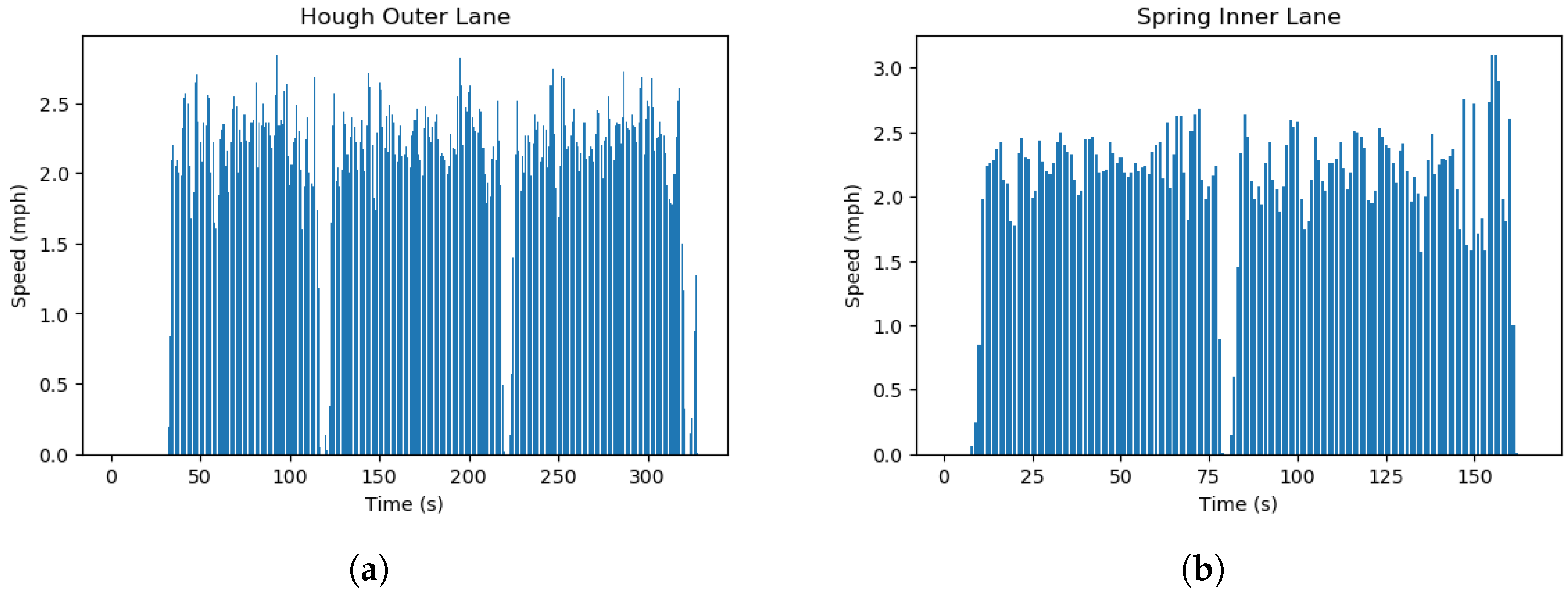
The speed control for the algorithms are noticeably more consistent than that of the human drivers as seen in Figure 25. The bumps in the graph are the result of the vehicle trying to make corrections for bumps and inconsistencies in the road. The sharp peaks and troughs of the graph are the result of losing a Hough line in the mask, then picking the line up again. The human drivers also demonstrated a tendency to go over the speed limit in many cases, suggesting it is difficult for humans to maintain a consistent speed at all times. On average, the human drivers were able to drive faster than the algorithms, close the set speed limit of seven miles per hour. However, the algorithms were not far off; the Hough algorithm was able to complete the outer lane laps at a maximum speed of 6.7 miles per hour and at an average speed of 4.476 miles per hour consistently for over four tests, which is comparable to the average speed of the human drivers. The human drivers would often exceed the speed limit and once they noticed the speed limit infraction on the speedometer of the vehicle, they would try to correct it by slowing down and the pattern would repeat throughout the laps for large distances traveled. On the other hand, the Hough algorithm for outer lane covered a much smaller distance of inconsistent change in speeds. Overall, the human driver was better at keeping to the lane at higher speeds, but struggled keeping a consistent speed when compared to the self-driving algorithms.

The algorithms are quite far from human performance in terms of control of the vehicle at high speeds though the Spring and Hough algorithm proved promising. In the recorded runs of the authors, the average speed ranged from 3.8 to 6.9 miles per hour (for each author attempting the course) when following the speed limit. In contrast, the Hough algorithm achieved an average speed of 4.476 miles per hour (and 4.358 miles per hour in another of the recorded runs) for outer lane which falls exactly within the range of the human runs.

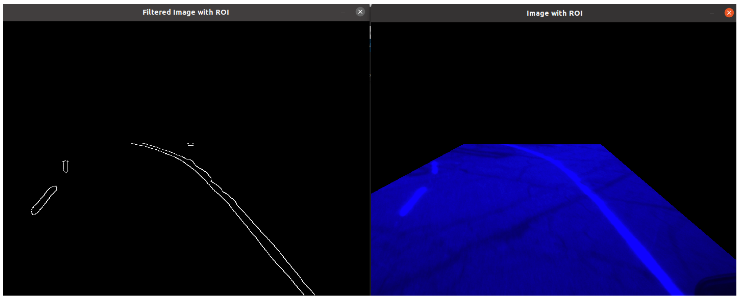
All of the algorithms faced some difficulty when under direct sunlight. Hough lines especially are dependent on the accuracy of the HSV (Hue, Saturation, Value) mask, which varies depending on weather and light conditions. The Hough algorithm performed best in overcast weather conditions. We observed that the spring algorithm had a superior performance for the inner lane when compared to the outer lane. We attribute this to the fact that the algorithm is able to better detect the lane when it is at a closer proximity to the vehicle due to the sharper curves.

Table 4. Table indicating the most difficult turn for each algorithm.

Parameter	Algorithm	Outer/ Inner	Location
Hardest Turn	Blob	Outer	Turn 2
		Inner	Turn 2 especially, but all turns are difficult
	Hough	Outer	Turn 3
		Inner	None, all face equal difficulty or ease
	Spring	Outer	None, all face equal difficulty or ease
		Inner	None, all face equal difficulty or ease

indicates the most difficult turn for each algorithm and Figure 26 provides the nomenclature to understand the table.

6. Conclusions

This research presented three different algorithms that autonomous vehicles may use to navigate both inner and outer roadway lanes. Real-world driving data and graphs showed that the human driver was better at staying within the lane while the algorithms excelled at driving at a certain speed consistently. We tested the algorithms on the ACTor self-driving platform as fast as they could go under the speed limit of seven miles per hour while still achieving the highest level of accuracy. In the end, during testing and demonstration, all three algorithms were able to complete the course for two laps. Some algorithms performed better than others, but ultimately, they were all able to complete the laps. Based on the results from all of the tables, we came to the conclusion illustrated in

Table 5. Summary of the findings.

Parameter Measured	Lane	Algorithm
Fastest Algorithm	Outer	Hough (max speed: 6.7 mph)
	Inner	Hough (max speed: 4.9 mph)
Smoothest algorithm/Algorithm with the least jerk	Outer	Hough
	Inner	Hough, Spring
Most reliable algorithm (based on the average success rate)	Outer	Hough
	Inner	Hough
Best overall algorithm/Most promising algorithm	Outer	Hough, Spring
	Inner	Hough, Spring

.

A high average speed, along with the minimal number of line touches, suggests good speed and centering control since it means the car did not have to slow down as much for turns. Existing lane-following algorithms are built for smooth, well marked roadways [7,9]. In this research work, despite the numerous obstacles, such as the tight curves and unmaintained roads, our algorithms were able to navigate the test course. These algorithms serve as a baseline for navigating the challenging sections of road.

Our work aims to enable a vehicle to drive under varied weather and road conditions without any human intervention within the bounds of a predefined course when the self-driving feature is enabled. As per SAE definition of autonomy (refer Figure 1), our work advances the computer vision aspect of self-driving research required to achieve full autonomy. However, we do not target a specific SAE level as our algorithms lack the capability for object detection, automatic emergency breaking, and warning systems. Hence, they do not comply with the standards defined in SAE J3016. Instead, our work focuses on making the lane detection algorithms work under less-than-ideal road conditions.

There are opportunities for future improvement of this study. For example, more data collection in the form of rosbags could be useful in getting more accurate values of the performance of the algorithms. We could also test the effectiveness of our filtration process under snowy conditions as long as the lanes are visible. The future directions of this research includes a fully-automated function to evaluate the performance of self-driving algorithms. We use an automated evaluation function to compute the time taken for the laps, the average speed, and the distance traveled over and below the speed limit. However, a fully automated evaluation system that also notes the weather conditions and number of line touches and departures could be built instead of any human evaluation. In addition, research into HDR (High Dynamic Range Imaging) algorithms can be used to improve the filtration pipeline used in this research as excessive sunlight and luminosity was a challenge that lead to a few failure cases (refer to Appendix A). Lane detection using deep learning algorithms such as LaneNet [12] followed by lane-centering algorithms could also be further explored.

The evaluation data files (or rosbags) of the algorithms driving are saved for further research in the future. The implementations of the algorithms are also open source and available on GitHub.

In the future, we intend to develop algorithms that will enable vehicles to travel faster and more accurately—ideally, at a pace that is equal to that of humans—and to deliver reliable data regardless of the weather, road conditions, or the amount of lighting present in the environment. We believe our work brings self-driving research one step closer to full automation.

References

1. SAE Levels of Autonomy. Available online: https://www.sae.org/blog/sae-j3016-update (accessed on 6 September 2022).
2. A Theoretician’s Guide to the Experimental Analysis of Algorithms. Available online: http://plato.asu.edu/ftp/experguide.pdf (accessed on 13 August 2022.).
3. Chung, C.-J. A Simple Lane-following Algorithm Using a Centroid of The Largest Blob, NSF Self-Drive REU 2022 Workshop at LTU. Available online: http://qbx6.ltu.edu/mcs/REU/workshop/lanefollowing_algo22chung.pdf (accessed on 30 July 2022.).
4. Matas, J.; Galambos, C.; Kittler, J. Robust Detection of Lines Using the Progressive Probabilistic Hough Transform. Comput. Vis. Image Underst. 2000, 78, 119–137. [Google Scholar] [CrossRef]
5. Paul, N.; Pleune, M.; Chung, C.; Warrick, B.; Bleicher, S.; Faulkner, C. ACTor: A Practical, Modular, and Adaptable Autonomous Vehicle Research Platform. In Proceedings of the 2018 IEEE International Conference on Electro/Information Technology (EIT), Rochester, MI, USA, 3–5 May 2018; pp. 0411–0414. [Google Scholar] [CrossRef]
6. Yenikaya, S.; Yenikaya, G.; Düven, E. Keeping the vehicle on the road: A survey on on-road lane detection systems. ACM Comput. Surv. 2013, 46, 1–43. [Google Scholar] [CrossRef]
7. Assidiq, A.A.; Khalifa, O.O.; Islam, M.R.; Khan, S. Real time lane detection for autonomous vehicles. In Proceedings of the 2008 International Conference on Computer and Communication Engineering, Kuala Lumpur, Malaysia, 13–15 May 2008; pp. 82–88. Available online: https://ieeexplore.ieee.org/abstract/document/4580573 (accessed on 13 July 2022). [CrossRef]
8. Devane, V.; Sahane, G.; Khairmode, H.; Datkhile, G. Lane Detection Techniques using Image Processing. In Proceedings of the ITM Web Conference, Navi Mumbai, India, 14–15 July 2021; Volume 40, p. 03011. [Google Scholar] [CrossRef]
9. Haque, M.R.; Islam, M.M.; Alam, K.S.; Iqbal, H.; Shaik, M.E. A Computer Vision based Lane Detection Approach. Int. J. Image Graph. Signal Process. 2019, 11, 27–34. [Google Scholar] [CrossRef] [Green Version]
10. Vajak, D.; Vranješ, M.; Grbić, R.; Teslić, N. A Rethinking of Real-Time Computer Vision-Based Lane Detection. In Proceedings of the 2021 IEEE 11th International Conference on Consumer Electronics (ICCE-Berlin), Berlin, Germany, 15–18 November 2021; pp. 1–6. [Google Scholar] [CrossRef]
11. Yang, J.; Wang, C.; Wang, H.; Li, Q. A RGB-D Based Real-Time Multiple Object Detection and Ranging System for Autonomous Driving. IEEE Sens. J. 2020, 20, 11959–11966. [Google Scholar] [CrossRef]
12. Wang, Z.; Ren, W.; Qiu, Q. LaneNet: Real-Time Lane Detection Networks for Autonomous Driving. arXiv 2018, arXiv:1807.01726. [Google Scholar]
13. Timmis, I.; Paul, N.; Chung, C.-J. Teaching Vehicles to Steer Themselves with Deep Learning. In Proceedings of the 2021 IEEE International Conference on Electro Information Technology (EIT), Mt. Pleasant, MI, USA, 14–15 May 2021; pp. 419–421. [Google Scholar] [CrossRef]
14. Jiang, Y.; Gao, F.; Xu, G. Computer vision-based multiple-lane detection on straight road and in a curve. In Proceedings of the 2010 International Conference on Image Analysis and Signal Processing, Zhejiang, China, 9–11 April 2010; pp. 114–117. [Google Scholar] [CrossRef]
15. McCall, J.C.; Trivedi, M.M. An integrated, robust approach to lane marking detection and lane tracking. In Proceedings of the 2004 IEEE Intelligent Vehicles Symposium, Parma, Italy, 14–17 June 2004; pp. 533–537. [Google Scholar] [CrossRef] [Green Version]
16. Andrei, M.-A.; Boiangiu, C.-A.; Tarbă, N.; Voncilă, M.-L. Robust Lane Detection and Tracking Algorithm for Steering Assist Systems. Machines 2021, 10, 10. [Google Scholar] [CrossRef]
17. Li, Y.; Iqbal, A.; Gans, N. Multiple lane boundary detection using a combination of low-level image features. In Proceedings of the 2014 17th IEEE International Conference on Intelligent Transportation Systems—TSC 2014, Qingdao, China, 8–11 October 2014. [Google Scholar] [CrossRef]
18. Cumali, K.; Armagan, E. Steering Control of a Vehicle Equipped with Automated Lane Centering System. In Proceedings of the 2019 11th International Conference on Electrical and Electronics Engineering (ELECO), Bursa, Turkey, 28–30 November 2019; pp. 820–824. [Google Scholar] [CrossRef]
19. Guo, J.; Wei, Z.; Miao, D. Lane Detection Method Based on Improved RANSAC Algorithm. In Proceedings of the 2015 IEEE Twelfth International Symposium on Autonomous Decentralized Systems, Taichung, Taiwan, 25–27 March 2015; pp. 285–288. [Google Scholar] [CrossRef]
20. Wang, Y.; Shen, D.; Teoh, E.K. Lane detection using spline model. Pattern Recognit. Lett. 2000, 21, 677–689. [Google Scholar] [CrossRef]
21. Ltu-Ros. LTU-Ros/Simple-Sim-Roads. GitHub. Available online: https://github.com/ltu-ros/simple_sim_roads (accessed on 24 June 2022).
22. Automatic White Balancing with Grayworld Assumption. Stack Overflow. Available online: https://stackoverflow.com/questions/46390779/automatic-white-balancing-with-grayworld-assumption (accessed on 24 June 2022).
23. Color Conversions. OpenCV. Available online: https://docs.opencv.org/3.4/de/d25/imgproc_color_conversions.html (accessed on 24 June 2022).
24. Canny, J. A Computational Approach to Edge Detection. IEEE Trans. Pattern Anal. Mach. Intell. 1986, PAMI-8, 679–698. [Google Scholar] [CrossRef]
25. Paul, N. Minimal Python Implementation of Blob Lane-Following Algorithm. Available online: https://github.com/nick-paul/lane_follow_blob (accessed on 12 August 2022.).
26. Duthon, P.; Bernardin, F.; Chausse, F.; Colomb, M. Methodology Used to Evaluate Computer Vision Algorithms in Adverse Weather Conditions. Transp. Res. Procedia 2016, 14, 2178–2187. [Google Scholar] [CrossRef] [Green Version]
27. Pappas, G.; Siegel, J.E.; Politopoulos, K.; Sun, Y. A Gamified Simulator and Physical Platform for Self-Driving Algorithm Training and Validation. Electronics 2021, 10, 1112. [Google Scholar] [CrossRef]
Figure 1. Levels of Driving Automation as defined by SAE J3016, revised in 2021. Source [1].
Vehicles 04 00055 g001
Figure 2. Environment: (a) One-to-one map of the test course in Parking Lot H used in simulation. The width of the lane, width of the road, radius for the turns, etc. are labelled in the above figure; (b) Bird’s-eye view of the test course in Parking Lot H at Lawrence Technological University.
Vehicles 04 00055 g002
Figure 3. The above images contain details about the vehicle: (a) ACTor Specifications. The width of the vehicle is 55.5 inches (141 cm) and length is 103 inches (262 cm) as labelled above; (b) The camera of the vehicle is fitted with sunglasses to reduce bright reflection and unwanted glare.
Vehicles 04 00055 g003
Figure 4. Flow chart of ROS node architecture generated using the rqt_graph plugin in ROS.
Vehicles 04 00055 g004
Figure 5. Filtration to detect yellow lines.
Vehicles 04 00055 g005
Figure 6. Mathematics behind the color conversion from RGB to CIELAB and RGB to HLS. Images sourced from [23].
Vehicles 04 00055 g006
Figure 7. The mathematics behind the operation of Canny Edge Detection is shown in the equations above.
Vehicles 04 00055 g007
Figure 8. Image after applying all the filters.
Vehicles 04 00055 g008
Figure 9. Image after applying Region of Interest function.
Vehicles 04 00055 g009
Figure 10. The above image shows the algorithm in action in 2 different simulators, namely SimpleSim and Gazebo. The circle is drawn at the centroid of the largest contour (the detected white line): (a) In SimpleSim simulator; (b) In Gazebo simulator.
Vehicles 04 00055 g010
Figure 11. This is a still from the camera of the vehicle when using the blob detection algorithm in the real time environment. As seen in the above figure, the largest white contour is found (marked in red) and the blue dot indicates the centroid of it. The ROI cropping is also seen above. (a) Outer lane; (b) Inner lane.
Vehicles 04 00055 g011
Figure 12. Pseudocode for the Yaw Rate calculation algorithm.
Vehicles 04 00055 g012
Figure 13. The Hough Lines and the Center Lane Line are visually represented in 2D simulation: (a) Average middle line lane; (b) Offset right line.
Vehicles 04 00055 g013
Figure 14. Hough Lines and Contour Detection. This is an image from the implementation of the algorithm in the real-time environment. The above figure shows the Hough Lines for the white lines drawn in blue and the center lane line drawn in red. Red was chosen as the color for the center line as red is not typically found on roads. The green on the red line indicates the Contour Detection of the center line. (a) Outer lane; (b) Inner lane.
Vehicles 04 00055 g014
Figure 15. Hough Lines and Average Center Lane Line. The ROI in Figure 17 is used for this method so that the white lines on both sides are detected. Both of these lines are used to create a fictitious center line which is shown in red. (a) Outer lane; (b) Inner lane.
Vehicles 04 00055 g015
Figure 16. The ROI used for Algorithm II when using the offset method of lane centering. Different ROIs are used for inner and outer lane: (a) Outer lane; (b) Inner lane.
Vehicles 04 00055 g016
Figure 17. The above image shows the ROI used for Average Center Lane Line method for lane centering. The same ROI is used for inner and outer lane.
Vehicles 04 00055 g017
Figure 18. The above image shows the working of the algorithm in simulation. The blue lines indicate the Hough lines and the yellow point indicates the center of the lane. The rays are extended until they touch the Hough lines on either side.
Vehicles 04 00055 g018
Figure 19. Visual Representation of the Hough Lines and the center point. The rays are drawn out to meet the Hough lines. The inner lane image shows how the algorithm works even on a sharp turn. (a) Outer lane; (b) Inner lane.
Vehicles 04 00055 g019
Figure 20. The above figure indicates the ROI cropping performed. Since both white lines are ideally required for this algorithm, the ROI is symmetrical on both sides.
Vehicles 04 00055 g020
Figure 21. The Lot H Course contains many broken lines where there should be solid lane lines. This mimics real-life, worn road conditions: (a) Broken white lane line is shown in the above image. The deteriorated road conditions are also seen; (b) A strip of reflective white tape is secured creating a more stable line to detect and track.
Vehicles 04 00055 g021
Figure 22. The above images indicate some of the environmental challenges faced. The images are from the test course. (a) Yellow parking lines near the lane interfering with yellow line detection; (b) Shadows from nearby trees interfering with lane detection.
Vehicles 04 00055 g022
Figure 23. Rainfall leaves reflective puddles across the course making it difficult to detect and track lane lines. Consistent rainfall on the windshield also caused multiple disturbances with camera consistency.
Vehicles 04 00055 g023
Figure 24. The above images show the speed-time graph for the best human drivers for inner lane and outer lane. The time taken, distance traveled above the speed limit, and average speed were taken into account for determining the best human driver.
Vehicles 04 00055 g024
Figure 25. The speed time graphs for Spring algorithm run on the inner lane and Hough algorithm on the outer lane are shown in the above images. For more graphs of the algorithms, please refer to Appendix A.
Vehicles 04 00055 g025
Figure 26. The nomenclature for the Turn Number is indicated in the above image.
Vehicles 04 00055 g026