Driving Robot for Reproducible Testing: A Novel Combination of Pedal and Steering Robot on a Steerable Vehicle Test Bench

Abstract

Shorter development times, increased standards for vehicle emissions and a greater number of vehicle variants result in a higher level of complexity in the vehicle development process. Efficient development of powertrain and driver assistance functions under comparable and reproducible operating conditions is possible on vehicle test benches. Yet, the realistic simulation of real driving environments on test benches is a challenge. Current test procedures and new technologies, such as Real Driving Emission tests and Autonomous Driving, require a reproducible and even more detailed simulation of the driving environment. Due to this, the simulation of curve driving in particular is gaining in importance. This results from its significant influence on energy consumption and Autonomous Driving functions with lateral guidance, such as lane departure and evasion assistance. Reproducibility can be additionally increased by using a driving robot. At today’s vehicle test benches, pedal and shift robots are predominantly used for longitudinal dynamic tests in the performed test procedures. In order to meet these new test automation requirements for vehicle test benches, the cooperative operation of pedal and steering robots is needed on a test bench setup suitable for this purpose. In this publication, the authors present the setup of a vehicle test bench to be used in automated and reproducible vehicle-in-the-loop tests during steering events. The focus is on the test-bench-specific setup with steerable front wheels, the actuators for simulating the wheel steering torque around the steering axle and the robots used for pedals and steering wheel. Results from various test series are presented and the potential of the novel test environment is shown. The results are reproducible in various test series due to the closed-loop operation without human driving influences at the test bench.

1. Introduction

In the vehicle development process, high reproducibility of tests is essential for identifying optimization potential. Tests on vehicle test benches therefore require trained and, above all, experienced drivers. However, the ability of the drivers to be reproducible is limited and also depends on the daily driver condition [1,2]. Due to currently prevailing topics such as Real Driving Emission (RDE) tests or Autonomous Driving (AD), cornering is also gaining in importance [3]. A test bench suitable for such tests must permit steering movements of the vehicle and should be able to realistically simulate the associated forces in the longitudinal and lateral directions.

For the driver, this requires transverse control of the vehicle position in a simulated driving scenario using the steering wheel, while simultaneously using the pedals for longitudinal control. Reproducible testing is thus an even greater challenge for the driver. While the human driver, for driving cycles such as the Worldwide harmonized Light-duty vehicles Test Cycle (WLTC), is supported by a $v\left(t\right)$-diagram on a driver guidance system, the support for more complex scenarios including steering movements is challenging. The driver can be supported by visualizing additional objects within the simulated driving scenario. Additional objects can be traffic signs, road users driving ahead, or a ghost vehicle representing the desired target position of the vehicle (Figure 1).

However, none of these visualization options can display all target values simultaneously. At least one target value cannot be represented, as shown in

Table 1. Possible options for the visualization of target values for the human driver.

	$\mathit{v}\left(\mathit{t}\right)$-Diagram	Traffic Signs	Vehicle Ahead	Ghost Vehicle
Velocity	x	x	x	x
Acceleration	x		x	x
Trajectory			x	x
Predictive driving	x	x

. Only a combination of different types can be used for a total target value representation. Nevertheless, sufficient stimulation of all target values is not guaranteed.

These challenges for reproducible testing result in the need for a higher-quality test environment through a higher level of test bench automatization without human driver influence. Such a test environment can consist of a steerable vehicle test bench as well as of controlled pedal and steering robots.

In this paper, the setup of a suitable vehicle test bench is presented, which has a combined pedal and steering robot and allows steering movements of the vehicle. The focus is on the technical implementation of this setup and on the control approaches of the driving robot. With the help of suitable test runs, results of the driving robot are compared with test bench drivers in order to confirm the suitability of this setup. At the end, an outlook is given as to which optimizations are necessary and which investigations are possible with this test bench in the future. In the following section, the current state of the art and research of vehicle test benches as well as of pedal and steering robots is shown.

2. Related Work

2.1. Steerable Vehicle Test Benches

For vehicle test benches, a general distinction can be made between chassis dynamometer and power train test benches. The chassis dynamometer is the most common type. These test benches can be used, for example, for exhaust gas or acoustic measurements [4] and consist of up to four rollers, which simulate driving resistance torque (street load) depending on speed, acceleration, and slope. The Vehicle under Test (VuT) stands with its tires on the crest of the rollers and is fixed via a hook fixation or a wheel hub fixation. Due to this construction, standard rollers cannot effect a steering motion of the VuT. For testing Advanced Driving Assistance Systems (ADAS) or AD functions, the ability to steer on a vehicle test bench has gained in importance. Many of the ADAS functions include lateral control and thus a steerable front axle on the vehicle test benches. For this reason, a novel test bench was introduced first by [5,6,7,8]. At this test bench, each tire of the VuT is mounted on a rotating double roller on which the tires can roll and steer at the same time.

In contrast to this, powertrain test benches have significant advantages due to their basic design, which allows adaptation in terms of steerability. These test benches are designed by each wheel hub being connected to the respective load engine. This allows to set the driving resistance for each wheel individually and to realistically simulate the load shift of the outer and the inner wheel. However, the wheels have to be removed for the powertrain test bench so that the wheel hubs can be connected to the load engine shafts. This demands a very accurate tire simulation in order to obtain comparable results with the real road tests. To enable steerabilty for these kind of test bench, there are different options, as described in [9]: Setting the front axle on a movable structure or disengaging the vehicle’s steering system and replacing it with a steering force module. The disengagement enables the force module to simulate the aligning or bore torque of the tire-track interaction, when the transfer path between tire and steering rack is realistically considered. As a result, the steering capability of this test technology can also be implemented more easily than on roller chassis dynamometers.

2.2. Pedal Robots

Pedal robots are used to reach a higher quality of test reproducibility in order to minimize the driver’s influence on the exhaust gas values [1,2,10,11,12]. Another advantage is to save costs, since no human test drivers are necessary. Further advantages are the relief of the human during demanding tests, such as endurance or climatic tests [13,14,15], or the improved ability to analyze data due to more reproducible driving [16]. In 1998, the German and US automotive industries defined requirements for pedal robots. An analysis of the pedal robots’ reproducibility compared to human drivers showed that humans drive with a higher tolerance than driving robots. Accordingly, the American Industry/Government Emissions Research set a lower limit for the Root Mean Squared Speed Error (RMSSE) for driving robots than for humans [1].

Since the driving behavior proved to depend on the vehicle characteristics [1] as well as on the selected vehicle mode [2], different control methods for pedal robots have been developed. An overview of the used control methods, required input parameters, and types of parameterization is presented in

Table 2. Pedal robot control methods, required input parameters, and types of parameterization used by different authors.

		[1]	[2]	[10]	[11]	[13,17,18,19]	[14]	[15]	[16]	[20]
Input parameters	Velocity	x	x	x	x	x	x	x	x	x
	Engine speed	x		x		x	x		x	x
Parameterization	Pre-learning cycles	x			x					x
	Technical data parameterization					x				x
	Learning while main cycle	x		x	x	x		x	x
	Not specified		x				x
Controller type	H-infinity				x
	PI				x	x		x
	PID									x
	Fuzzy		x					x
	Vehicle model			x		x
	Not specified	x					x		x

.

All authors used the vehicle velocity as an input variable for the longitudinal control. Some authors additionally considered engine speed within the control algorithm. The type of parameterization varies between manual parameterization (teach-in phase), partial with additionally required test cycles and self-learning approaches during the main tests. Since teach-in phases are time-consuming [1], the authors in [16] implemented a self-learning system for learning the vehicle behavior. The authors in [13,17,18,19] alternatively designed a universal vehicle model for the longitudinal control. The required parameterization process with common vehicle parameters reduces the teach-in phase to referencing the actuators when the motor is switched off [12]. In this vehicle model [13,17,18,19], the braking system was not modeled, since the behavior of the composition of braking force support, ABS and ESP is different for each vehicle. However, the authors noted that brake pedals always have an idle distance and decelerations $<0.5 \mathrm{m}/{\mathrm{s}}^2$ mostly result from drag torque. For larger decelerations, a linear relationship between brake pedal displacement and deceleration can be assumed. Furthermore, the authors emphasized that the brake is a safety aspect of the driving robot to transfer the vehicle into a safe operating condition. The authors in [19] also mentioned that oscillations in the accelerator pedal should be avoided; otherwise, increased emission levels will result. Most authors used a PI or PID control method. The authors in [20] used one PID controller for both throttle and brake, positive values for the accelerator pedal and negative values for the brake pedal. A dynamic fuzzy neural network direct inverse control with self-learning of vehicle longitudinal performance in combination with a PI controller for compensation of the approximation error of the direct inverse controller was used in [15]. According to the authors, this gave better results compared to PID control or pure fuzzy control. Furthermore, the authors in [2] compared a PI controller with a fuzzy logic PI controller at different vehicle modes (Eco and Sport). By using a fuzzy logic PI controller, the RMSSE was reduced by more than $30\%$ compared to a PI controller. In addition, deviations from the target speed became smaller at speeds greater than $60 \mathrm{k}\mathrm{m}/\mathrm{h}$. A look-ahead time was used in [10] since tests with experienced drivers revealed that they also need a look-ahead time of at least $1 \mathrm{s}$. The authors in [1] added that driving robots without look-ahead time are not more reproducible than humans.

In many cases, the used hardware components of the driving robots consisted of the throttle, brake, clutch, and gearshift with individual actuators [10,11,12,19]. The authors in [20] used one motor for both throttle and brake, due to the non-simultaneous use of throttle and brake. Linear actuators in particular are used in [12,14]. The authors in [14] specifically focused on spindle-free, electromagnetic linear actuators and showed their advantages over other types of pedals. For hybrid electric vehicles, ref. [2] used a different approach by manipulating CAN signals instead of using actuators for control. This is only possible without further effort if the vehicle has an electric brake pedal.

2.3. Driving Robots: Pedal and Steering Robots

In the early 2000s, there was interest in autonomous vehicles for reproducible testing on extreme test tracks [21]. For this purpose, a combination of a pedal and steering robot was developed. A driving trajectory and velocity profile was generated using a multisensor perception platform. Similar to other approaches, the pedal robot is characterized by three actuating levers for gas, brake, and clutch. Steering was realized by a lever, which was rigidly connected to the steering wheel. Moreover, there were additional levers to change the gears and start the engine. The same mechanical design was also used in [16,22]. The latter used model predictive control for lateral guidance, based on a two-wheel two-degrees-of-freedom steering model. Target trajectory, steering speed, driving speed, and driving acceleration all served as input for the control of longitudinal and lateral directions. Path planning, which was based on a perception unit as well as the vehicle’s kinematics and dynamics, resulted in the target trajectory. The authors in [23] only used two motors for the steering wheel and the pedals, with the accelerator and brake pedals being controlled together by one motor. Furthermore, longitudinal and lateral dynamic controllers were also separated to simplify the system. However, both are based on cascaded PID controllers with velocity and yaw error as inputs. An inertial measurement unit was used to calculate the motion and position data.

Another field of application is presented in [24]. Here, the combination of a pedal and steering robot is used for testing emergency braking assistants for pedestrians to provide a realistic simulation of critical scenarios. As this application was part of the Chinese NCAP test, speed tolerances of $\pm 0.5 \mathrm{k}\mathrm{m}/\mathrm{h}$ had to be maintained. The robot consisted of a pedal robot for automatic vehicles controlled via pressure and position sensors in combination with a steering robot controlled via GNSS.

3. System Design

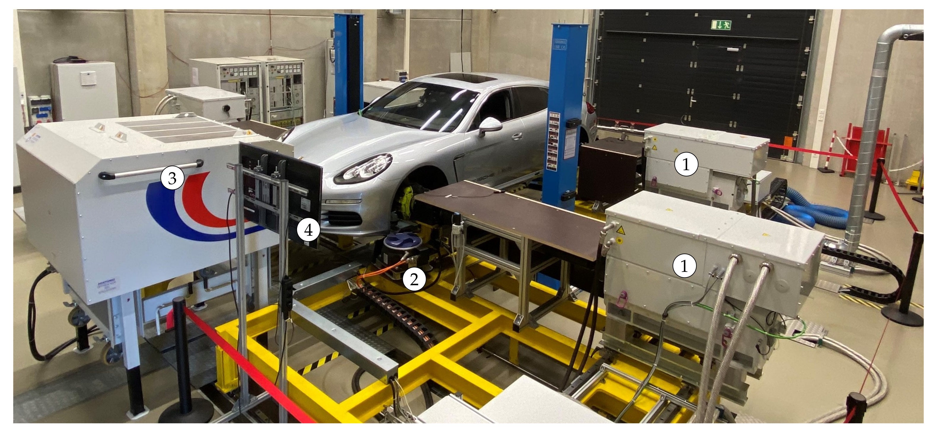
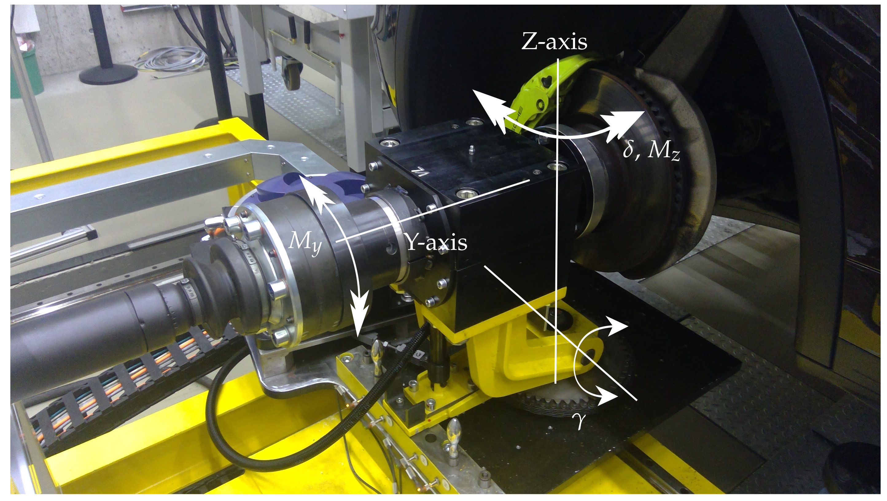
3.1. Vehicle-in-the-Loop Test Bench

The Vehicle-in-the-Loop Test Bench at the Institute of Vehicle System Technology (FAST) of the Karlsruhe Institute of Technology (KIT), shown in Figure 2, can be used for vehicle measurements in longitudinal and lateral dynamic driving situations. The hard- and software structures of the test bench are described in detail below.

3.1.1. Hardware Setup

The test bench consists of four three-phase synchronous machines (1) (Figure 2). These are mechanically connected to the four wheel flanges of the vehicle via four constant velocity drive shafts and four rotatably mounted wheel adapters (Figure 3), and can thus transmit forces and simulate the load-dependent driving resistances as well as the operating point relevant tire characteristics. The torque is measured directly at the connection between the wheel hub and wheel adapter, so that possible losses due to the shaft and load machine have no influence. The speed can be measured directly at the load machines due to the connection to the vehicle via constant velocity drive shafts. The load machines are fed by highly dynamic frequency converters. The rotatably mounted wheel adapters are mechanically connected to two additional synchronous machines at the front axle via a chain drive (2). These simulate the self-aligning torque that occurs at the wheels steered. The air fan (3), which ensures sufficient air flow for heat dissipation in the drive train, is located in front of the VuT. A screen next to the blower, the driver guidance system (4), allows the driver to follow driving instructions. The test stand is monitored on several screens in a separate control room using five cameras placed at the test bench. The main technical data of the test rig are given in

Table 3. Technical data of the test bench.

Description	Data
Nominal wheel load power	$209 \mathrm{k}\mathrm{W}$
Max. wheel load torque at nom. speed ($800/\min$)	$2500 \mathrm{N}\mathrm{m}$
Max. wheel speed	$2000/\min$ ($260 \mathrm{k}\mathrm{m}/\mathrm{h}$ with $r_{dyn}=0.34 \mathrm{m}$)
Max. self-aligning torque at the front wheels	$1000 \mathrm{N}\mathrm{m}$
Max. steering angle at the front wheels	$\pm 18{}^{\circ }$
Max. air fan wind speed	$135 \mathrm{k}\mathrm{m}/\mathrm{h}$
Max. vehicle weight	$\mathrm{12,000} \mathrm{k}\mathrm{g}$
Max. wheel load	$3000 \mathrm{k}\mathrm{g}$
Wheelbase	$1.8 \mathrm{m}$–$4.9 \mathrm{m}$
Track width	$1.2 \mathrm{m}$–$3.9 \mathrm{m}$

.

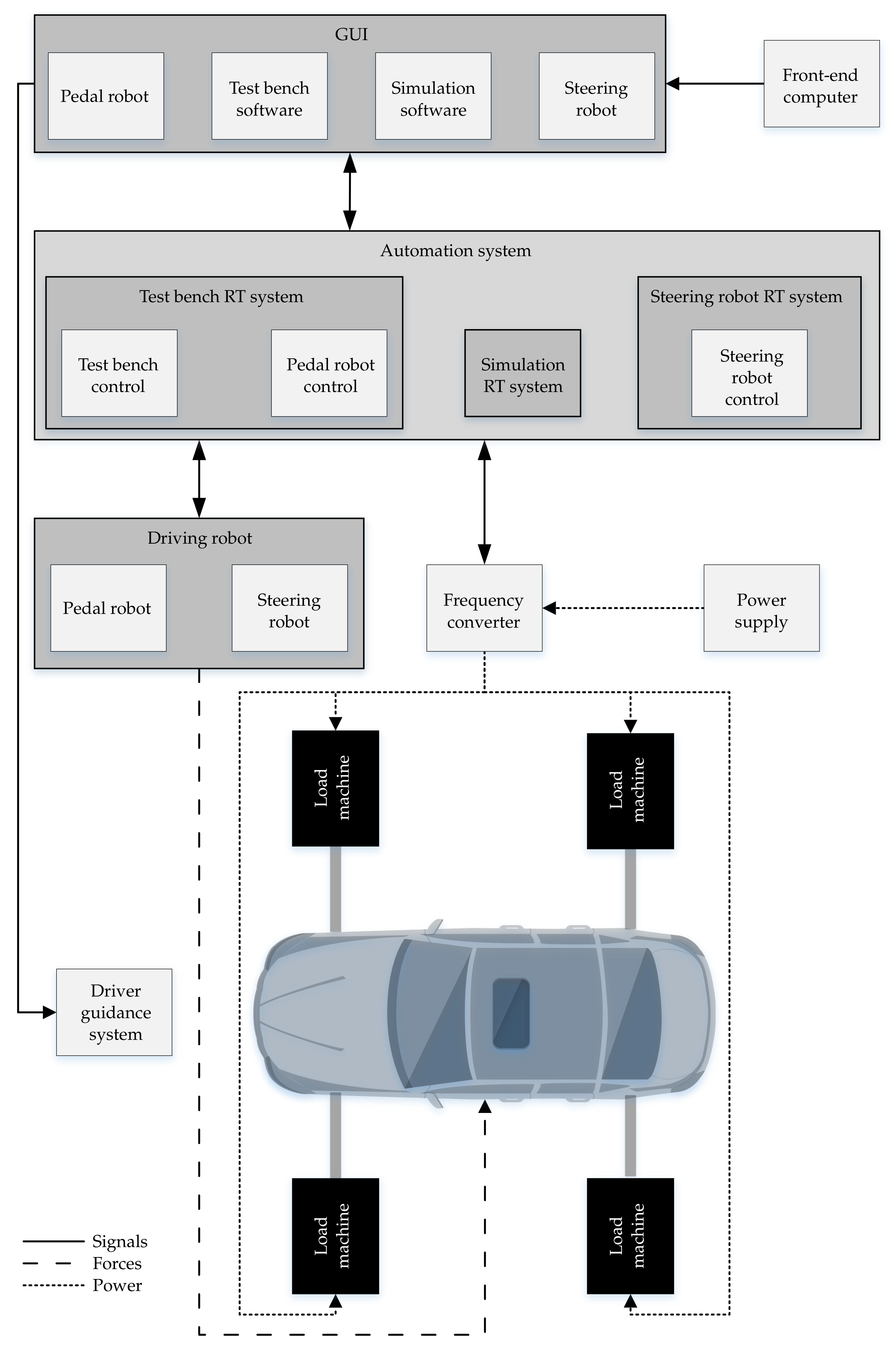
3.1.2. Software Setup

A real-time (RT) system is responsible for the software monitoring and control of the test bench. The communication between the RT system and controllers of individual components is mostly carried out via EtherCAT and partly via CAN. The control software is visualized to the end user via a Graphical User Interface (GUI) on a front-end computer. The following three test bench control modes are available for selection in the GUI:

• Velocity control (speed control)
• Driving resistance control (torque control)
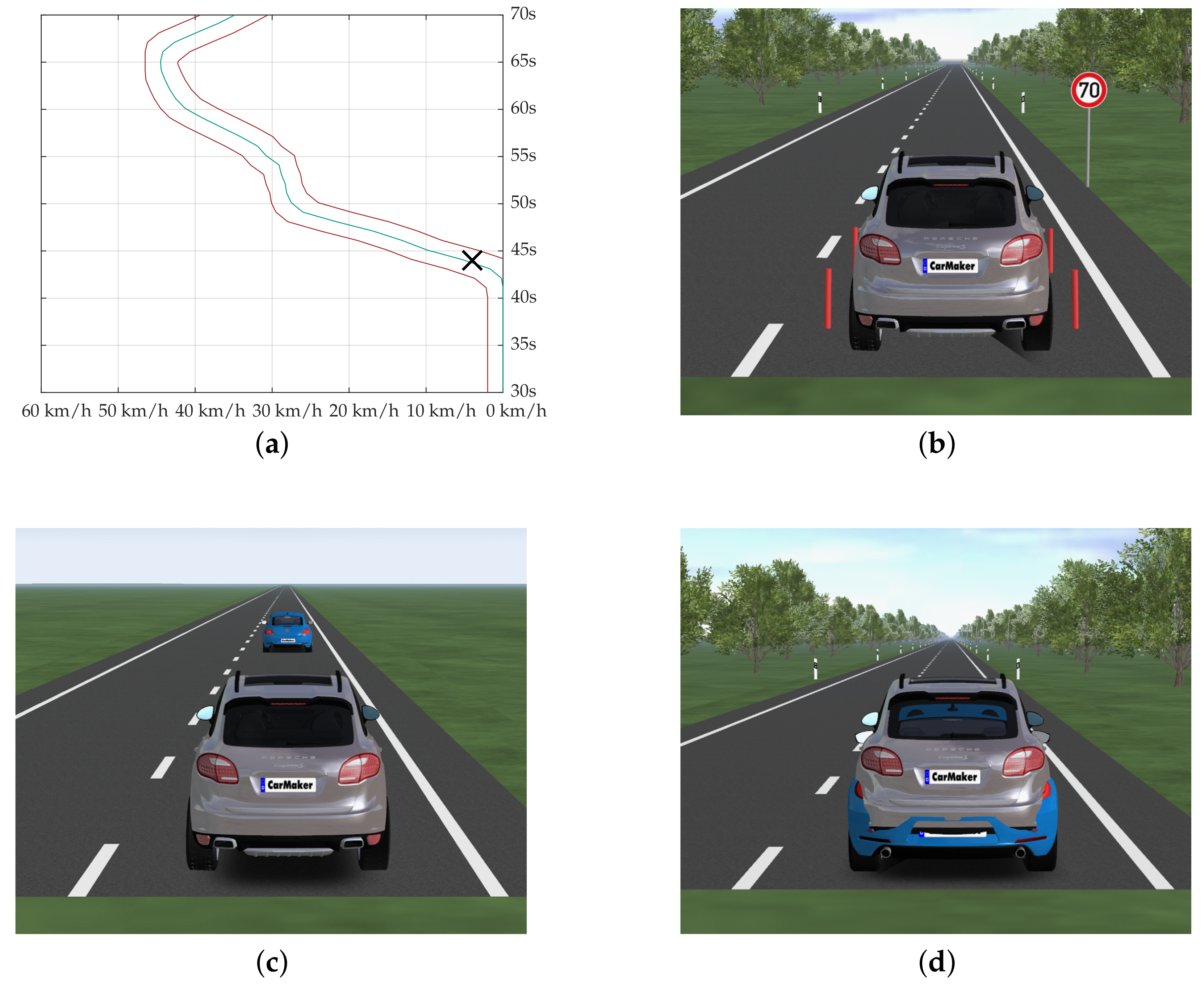
• Virtual real driving simulation with CarMaker (speed control)

In mode 1, a predefined speed is controlled by the test bench so that different loads on the drivetrain can be investigated at the same wheel speed. In mode 2, the wheel-dependent driving resistance is simulated under torque control depending on the vehicle speed, road slope, and individual vehicle parameters. The driving resistances simulated with the load engines can be calculated either by the corresponding Equations (1) to (5) based on the main parameters shown in

Table 4. Parameters and units of the shown driving resistance equations.

Description	Symbol	Unit
Drag coefficient	$c_w$	-
Projected frontal area	A	${\mathrm{m}}^2$
Air density	$\rho$	$\mathrm{k}\mathrm{g}/{\mathrm{m}}^3$
Vehicle mass	m	$\mathrm{k}\mathrm{g}$
Gravitational acceleration	g	$\mathrm{m}/{\mathrm{s}}^2$
Rolling resistance coefficient	$f_R$	-
Mass factor	$\lambda$	-

or by the coefficients of a coast down curve.

$$\begin{array}{cc}\hfill F_{Wheel}& =F_{air}+F_{roll}+F_{acc}+F_{slp}\hfill \end{array}$$

(1)

$$\begin{array}{cc}\hfill F_{air}& =\frac{1}{2}{c}_w·A·\rho ·v^2\hfill \end{array}$$

(2)

$$\begin{array}{cc}\hfill F_{roll}& =m·g·cos\alpha ·f_R\hfill \end{array}$$

(3)

$$\begin{array}{cc}\hfill F_{acc}& =m·a·\lambda \hfill \end{array}$$

(4)

$$\begin{array}{cc}\hfill F_{slp}& =m·g·sin\alpha \hfill \end{array}$$

(5)

The third mode involves the simulation software, CarMaker TestBed from IPG Automotive, and the related RT system. In this operation mode, consumption-relevant simulations of cornering are possible. In addition to the variables already mentioned, the steering angles of the two front wheels are also considered and the self-aligning torque as well as the increased driving resistances due to cornering [3] are simulated.

In all modes, the test bench RT system as part of the automation system communicates with the load machines via the frequency converters, as shown in Figure 4.

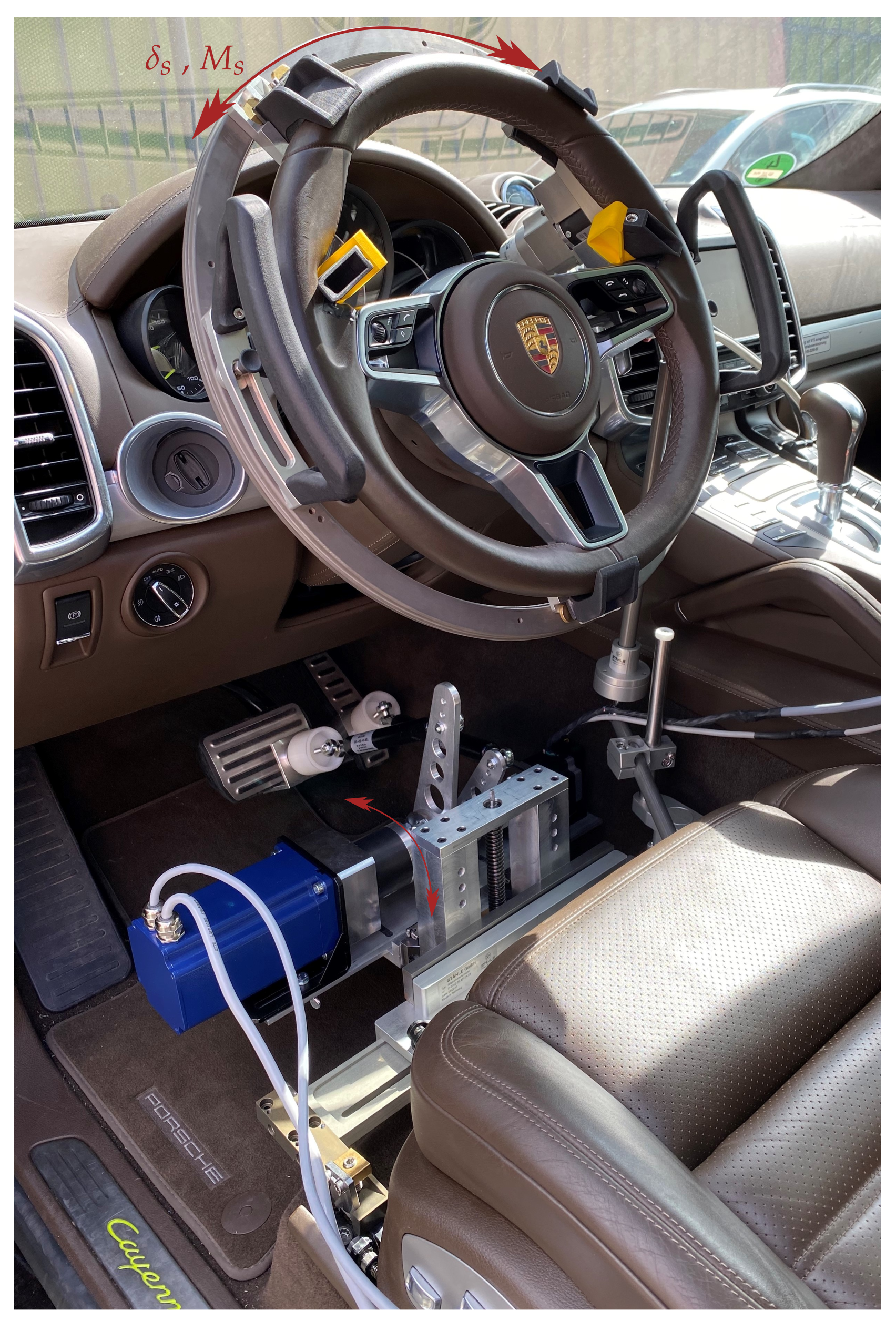
3.2. Driving Robot: Combination of a Pedal and Steering Robot

To carry out driving tests at the test bench, the combination of the steering and pedal robots shown in Figure 5 is used. These are integrated into the automation system of the test bench (Figure 4) and operate the vehicle in longitudinal and lateral dynamic directions. The hard- and software structures of the robots are described in detail in the following.

3.2.1. Hardware Setup

The steering robot is a product of Stähle GmbH. A steering ring including internal teeth is clamped to the steering wheel. Power is transmitted via an electric motor with a mounted gear wheel. The weight of the electric motor is held by a rod system on a mechanism fastened on the seat rails. The belonging control unit is integrated into the automation system of the test bench via CAN.

The pedal robot is an in-house development of KIT-FAST and can be used for vehicles with automatic transmission. Two motors actuate the accelerator and brake pedals. The rotational movement of the servomotors is converted into a compressive force via a lever arm and an attached rod. This force is clamped to the associated pedal via a screw connection. The servomotor for the brake pedal is larger in size, as increased forces are required for the brake pedal contrary to the accelerator pedal. The motors are positioned on a mechanism that can be moved in the longitudinal, transversal, and vertical direction to adapt the pedal robot to the respective vehicle. The mechanism of the pedal robot is connected to the mechanism of the steering robot on the seat rails and can thus be used in combination with the steering robot. The motor controllers are integrated into the automation system of the test bench via EtherCAT.

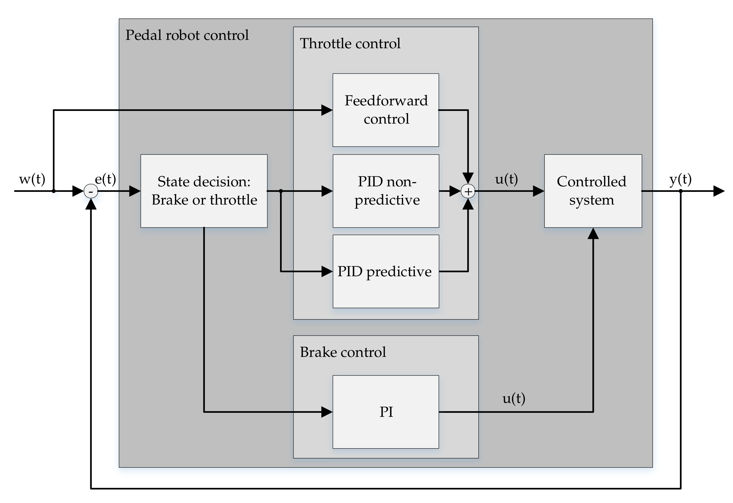
3.2.2. Software Setup

The operating mode of the steering robot can be selected via the front-end computer using a GUI. A decision can be made between two modes:

• Steering wheel angle control
• Virtual real driving simulation with CarMaker

In mode 1, a steering angle can be specified via the steering robot GUI, which is then adjusted by the control unit of the steering robot. In mode 2, the simulation calculates a steering wheel position for the virtual vehicle based on the selected steering system and on the current driving operation state in the virtual driving environment. For controlling the steering wheel angle, the lateral control of the IPGDriver is used. The steering wheel position is sent to the control unit as a target value and adjusted via the electric motor. By changing the steering wheel angle, the new angle of the wheels and thus the new position of the vehicle can then be determined and a new steering wheel position can be calculated.

The settings of the pedal robot can be entered via a further GUI. Specifically, the vehicle parameters and the selection of the operation mode are requested within this GUI. The following operation modes can be selected:

• Pedal control
• Velocity control
• Driving cycle control
• Virtual real driving simulation with CarMaker

In mode 1, the pedals will be actuated according to predefined pedal positions. For example, the vehicle’s response to pedal jumps or the behavior of the vehicle at certain pedal values in different driving scenarios (cornering, uphill slopes) can be investigated. In modes 2 and 3, the pedal position is controlled depending on the vehicle speed. The target values are taken either from a speed defined in the GUI (mode 2) or from the specification of an entire driving cycle (mode 3). Mode 4 can be used for both control and regulation. All functionalities of the first three operation modes can be covered in mode 4. In general, closed-loop operation is achieved by measuring the actual pedal position.

The control of the pedal robot is based on [19] and was adapted and further developed for the test bench at KIT-FAST. The overall structure of the pedal robot control model is shown in Figure 6. The three main components of the control are the throttle and brake pedal control, as well as the decision logic, which pedal is controlled. The latter, for example, is based on defined threshold values for the speed deviation, the target speed or the target acceleration. The pedal controls must also be differentiated. Brake pedal control is handled by a PI controller during driving. At standstill, the control is deactivated and a fixed pedal value is set to avoid oscillations. The throttle control has a more complex design due to the delayed response time of the controlled system (powertrain) compared to the brake system. A distinction is made between a feedforward, a non-predictive, and a predictive control component:

$$u\left(t\right)=u_{Feedforward}\left(t\right)+u_{PI{D}_{non-predictive}}\left(t\right)+u_{PI{D}_{predictive}}\left(t\right)$$

(6)

The feedforward control is based on the load point-dependent driving resistances, the vehicle inertias, and the full-load curve of the powertrain. For a detailed description of the control, refer to [19]. With precise knowledge of the vehicle, the feedforward control can regulate the pedals sufficiently well. However, this requires various information, such as the engine map, knowledge of the selected gear, etc. Since this information is not available in detail for every vehicle and can thus only be estimated, additional controllers are used. The non-predictive controller mainly corrects the feedforward control to avoid negative influences due to missing detailed information about the vehicle. The predictive controller is also used to overcome inertias in the powertrain, which can occur especially in vehicles with internal combustion engines. Both the predictive and the non-predictive control components are designed as PI or PID controllers:

$$u_{PID}\left(t\right)=K_P·e\left(t\right)+K_I·{\int }_0^{t}e\left(\tau \right)\mathrm{d}\tau +\underset{\mathbf{Throttle} \mathbf{control} \mathbf{only}}{\underbrace{K_D·\frac{\partial e\left(t\right)}{\partial t}}}$$

(7)

The two controllers have separate vehicle-dependent constants, $K_P$, $K_I$, and $K_D$, with separate look-ahead times of up to 2 s. The sum of the three controllers (Equation (6)) results in the required accelerator pedal position. The pedal that is not controlled receives a value of $0\%$ as the target value in each case.

The controls of the pedal and the steering robot, and thus the longitudinal and lateral control, are currently acting separately from each other. While the lateral control of the IPGDriver sets the steering wheel angle depending on the target trajectory and the speed, the longitudinal control follows a speed-time profile. The latter must therefore be designed for the respective route with the aid of physical relationships so that the vehicle decelerates sufficiently before curves.

4. Performed Test Cases

4.1. Test Case Definition

In order to evaluate the suitability of the pedal and steering robot on the steerable vehicle test bench, various test runs were used. The driving quality of the robot was compared with the quality of human drivers in these test runs. All tests were carried out on the Vehicle-in-the-Loop Test Bench of KIT-FAST. The following cycles were selected for the test runs:

• WLTC Class 3b (pedal robot)
• Steering circles (pedal and steering robot)
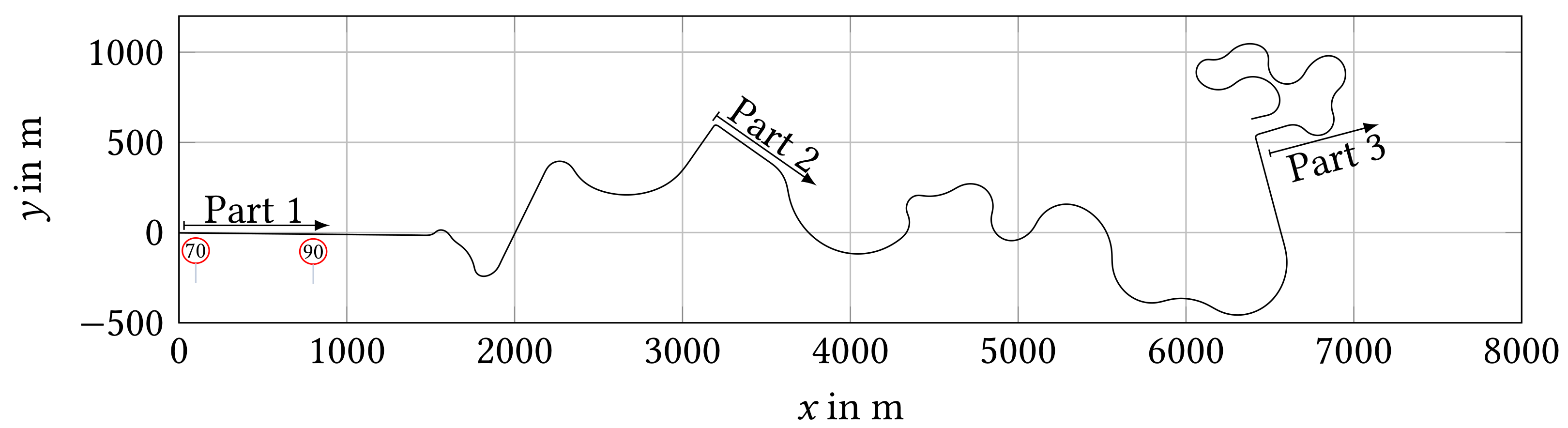
• Real driving cycles (pedal and steering robot)

The WLTC is mainly used in exhaust gas testing and therefore primarily on chassis dynamometers. Criteria with defined limit values, such as the RMSSE or the Inertial Work Rating (IWR), whose explanation follows in Section 4.2.1, make it suitable for evaluating longitudinal dynamic driving behavior. Thus, in the first step, the WLTC can be used to independently analyze the speed control of lateral dynamic influences.

In the next step, the trajectory follow-up control is analyzed in steering circles. Two constant radii with constant velocities, in order to be able to avoid any undesired effects, are used.

Finally, a section of a real driving route is used to investigate the interaction of longitudinal and lateral dynamics control with varying velocities and curve radii. The initial target velocity is set at $70 \mathrm{k}\mathrm{m}/\mathrm{h}$. After 600 m, the velocity increases to $90 \mathrm{k}\mathrm{m}/\mathrm{h}$ for the rest of the route. The curve angles reach up to $90{}^{\circ }$ on a route length of $12 \mathrm{k}\mathrm{m}$. The route can be split into different parts (see Figure 7): The route begins with a straight part containing a few corners to show the drivers’ (robot or human) different handling of a mostly straight route. The first part ends at the first $90{}^{\circ }$ corner. The second part also starts with a straight street and changes into a more curvy street. The third part of the real driving route begins with another $90{}^{\circ }$ angle corner and represents a curvy interurban part with small corners. Additional road users were not added to the route because the focus is placed on the road layout and not on the energy consumption in different traffic conditions or compositions. The main information about the different cycles can be taken from

Table 5. Performed cornering cases.

Test Case	Curve Radius	Vehicle Velocity
Steering circle	$r=50\mathrm{m}$	$v=50 \mathrm{k}\mathrm{m}/\mathrm{h}$
Steering circle	$r=80 \mathrm{m}$	$v=50 \mathrm{k}\mathrm{m}/\mathrm{h}$
Real driving	r $\ge 16 \mathrm{m}$	$v_{max}=90 \mathrm{k}\mathrm{m}/\mathrm{h}$

.

4.2. Test Results

Selected test runs of the robot and the human drivers were examined and are analyzed in this section in order to evaluate the driving quality of the robot.

4.2.1. WLTC

For the homologation tests, the RMSSE in a WLTC must be less than $1.3 \mathrm{k}\mathrm{m}/\mathrm{h}$ [25]. Comparing this limit with the values determined from the test runs in

Table 6. Determined WLTC limit values for selected test runs.

Driver	RMSSE in km/h	IWR in %
Human	1.86	4.38
Human	1.75	3.73
Human	1.25	6.25
Human	1.35	2.85
Human	1.14	2.70
Human	1.46	6.13
Robot	0.83	5.78
Robot	0.89	7.08

, four of the human test runs exceed this tolerance. Only three tests have a sufficient small RMSSE. In addition, the values for the RMSSE of the runs with the driving robot are significantly smaller than the RMSSE of runs with a human driver. These findings, and the smaller value range, already indicate the better driving behavior and reproducibility of the driving robot. The humans are drivers with medium to little driving experience on test benches. The driving behavior of experienced test bench drivers deviates from this.

The previously mentioned limit value IWR is not considered further in the following. The reason is the method of calculation. According to [26], only sections of positive acceleration are considered (except for vehicles with regenerative braking systems), which means that braking phases in particular are not taken into account. Furthermore, in contrast to the RMSSE, it is not the absolute values that are considered, but the pure checksum. This means that positive and negative energy differences (velocity deviations) can neutralize each other. An evaluation of the reproducibility over the entire cycle is therefore not completely possible. Nevertheless, the results with the positive values show that, on average, more energy is needed and thus the drivers tend to drive faster. The driving robot in particular is above the limit value of $4\%$ [25] in each of the tests carried out.

Considering the ratio of target and actual velocity in Figure 8, a larger dispersion can be derived for several human drivers (red triangles), especially at low velocities. Here, deviations of $>10 \mathrm{k}\mathrm{m}/\mathrm{h}$ occur in some cases. In particular, the starting phase or load changes represent a major challenge. In these areas, the driving robot (green circles) also shows optimization potential, but to a lesser extent than the human driver. In addition, the driving behavior of the driving robot is reproducible and the deviations from the target velocity at constant accelerations are negligible.

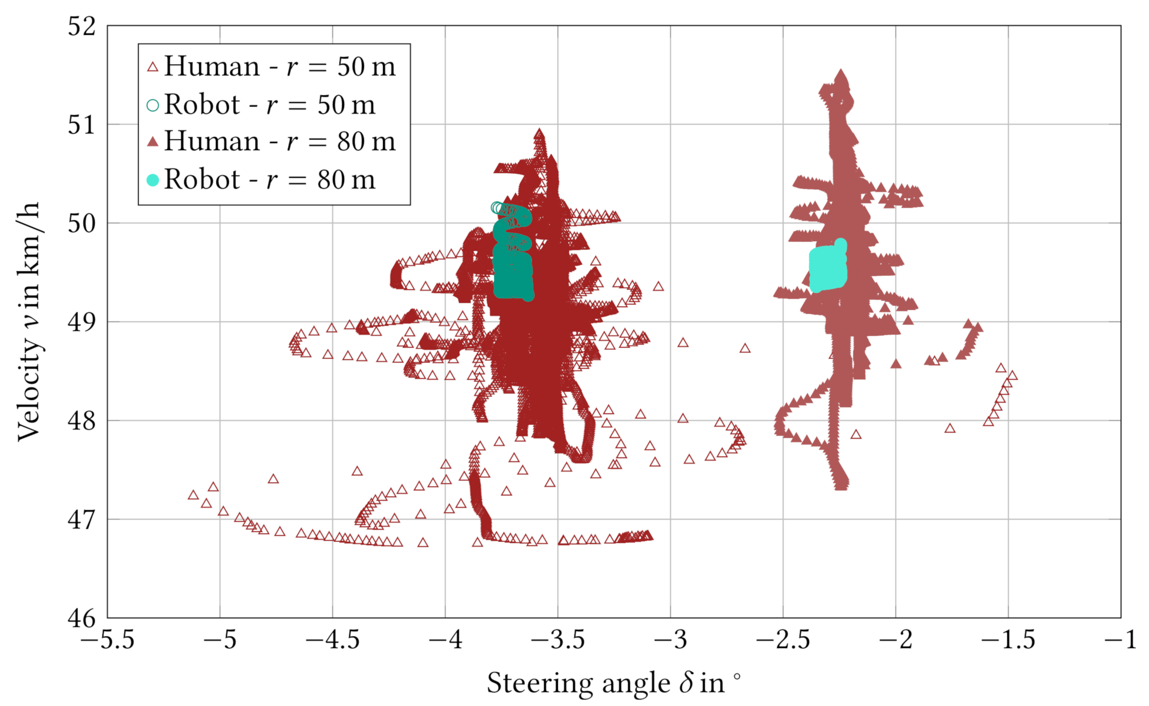
4.2.2. Steering Circle

Figure 9 summarizes the results of the circle runs. The speed deviations in the circles performed by the driving robot are comparable to the previously calculated values of the RMSSE. However, the human driver regulates with a tolerance of $\pm 2 \mathrm{k}\mathrm{m}/\mathrm{h}$ around the target speed and deviates up to $3.5 \mathrm{k}\mathrm{m}/\mathrm{h}$ from the target speed in some cases. In order to maintain the course, the robot adjusts the steering angle at the wheel and corrects this with a slight oscillation with an amplitude of approximately $0.05{}^{\circ }$ (radius $80 \mathrm{m}$, green-filled circle) or $0.1{}^{\circ }$ (radius $50 \mathrm{m}$, green circles). This oscillation can be attributed to play in the steering wheel, as well as measurement noise or measurement inaccuracies. In addition to the deviation in the longitudinal direction of the vehicle, the human driver also deviates more strongly in the transverse direction of the vehicle. Oscillations of $0.25{}^{\circ }$ (radius $80 \mathrm{m}$, red-filled triangles) and $0.35{}^{\circ }$ (radius $50 \mathrm{m}$, red triangles) are achieved. In addition, clear outliers of more than $2{}^{\circ }$ (radius $50 \mathrm{m}$) and approximately $0.6{}^{\circ }$ (radius $80 \mathrm{m}$) are recognizable. The larger the radius and thus the smaller the lateral forces or the steering angles, the better the human driver can control both target values. Nevertheless, the driving performance is not comparable to that of the driving robot, as the Root-Mean-Squared Error (RMSE) in

Table 7. RMSE from the nominal steering angle $\delta$ in the driven circles.

Driver	${\mathit{\delta }}_{\mathbf{RMSE}}$ ($\mathit{r}=80$ m)	${\mathit{\delta }}_{\mathbf{RMSE}}$ ($\mathit{r}=50$ m)
Human	$-0.0672{}^{\circ }$	$-0.1{}^{\circ }$
Robot	$0.0000084{}^{\circ }$	$0.0034{}^{\circ }$

also shows.

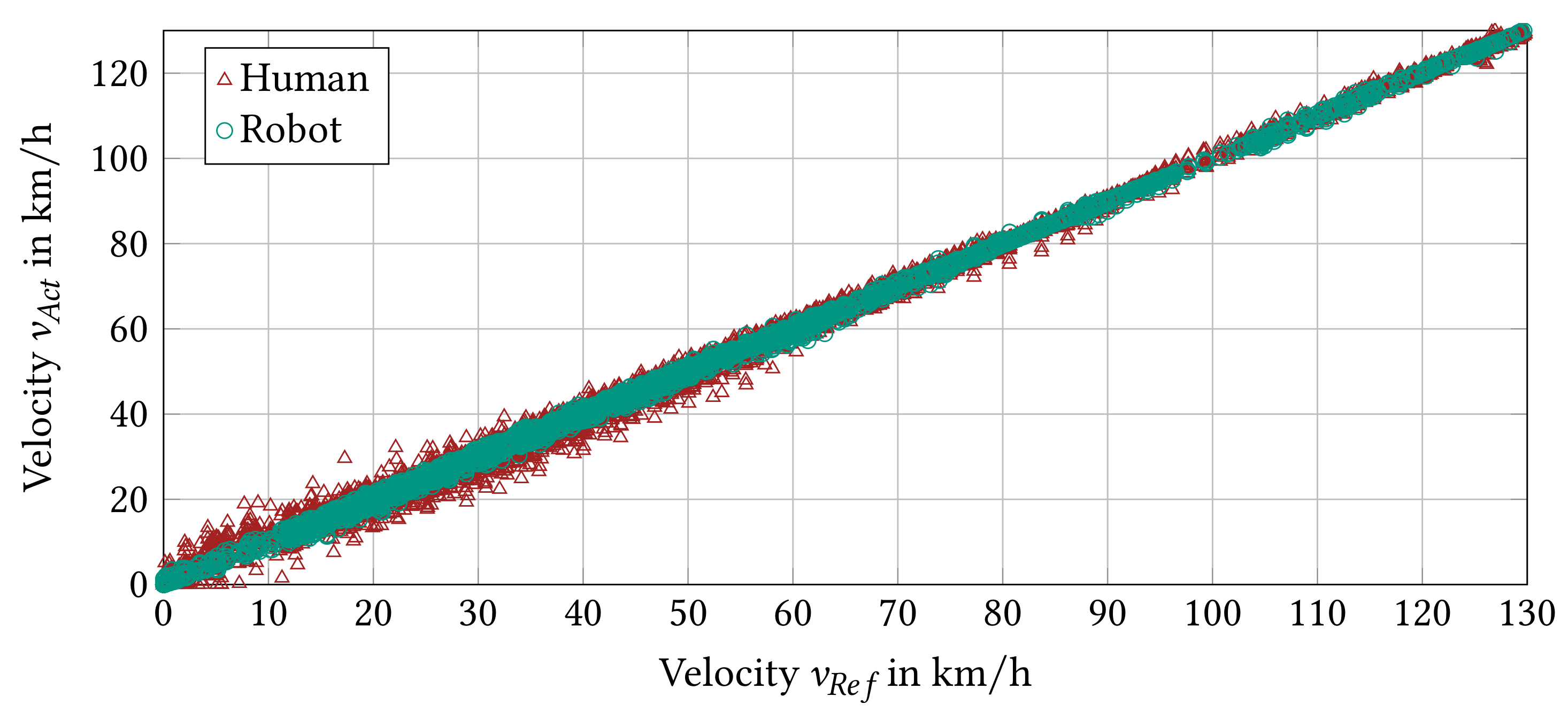
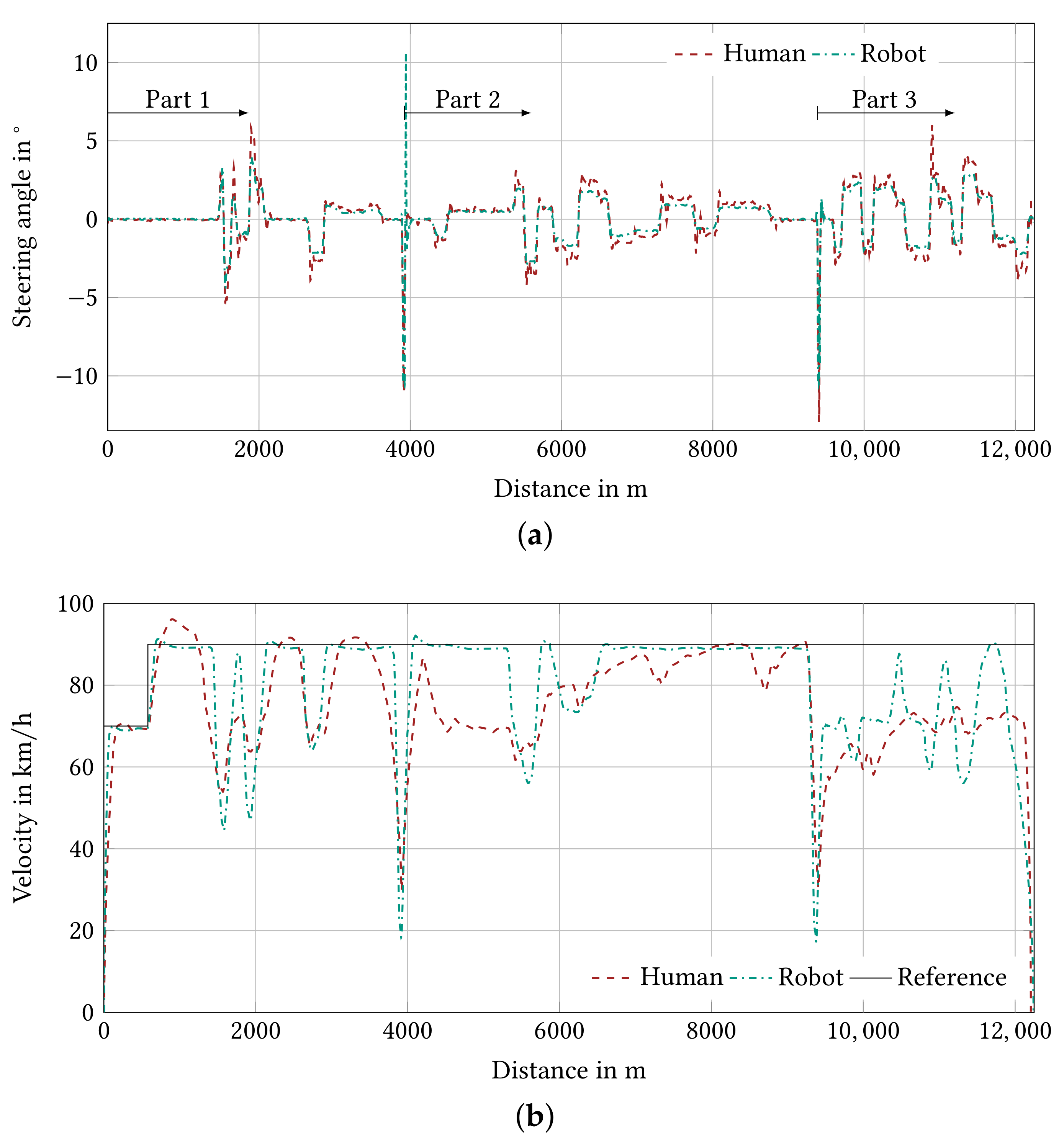
4.2.3. Real Driving Route

The measurement results of the virtual real driving route show that the human driver has significantly higher deviations from the target trajectory or target velocity in some cases during the driving maneuver (Figure 10). In the first section, the human driver accelerates slower and then beyond the target velocity. In the first deceleration phase at distance ∼$1400 \mathrm{m}$, the human driver operates the vehicle more predictively and thus brakes earlier with a lower deceleration. For the subsequent cornering at distance ∼$1700 \mathrm{m}$, the human driver makes larger steering movements compared to the driving robot and at the same time also deviates significantly from the target speed. In the $90{}^{\circ }$ curves at distances ∼$4000 \mathrm{m}$ and ∼$9500 \mathrm{m}$, the driving robot performs worse because it accelerates more dynamically out of the curves, resulting in extreme steering movements in some cases. In curves with constant curvatures, the human has increased difficulties in regulating the steering angle and speed in a balanced manner, as already shown in the results of the steering circles. In most cases, the speed decreases strongly. In summary, the human driver has problems managing speed and steering angle changes simultaneously. In these cases, the driving robot is more accurate and consistent.

4.3. Discussion

The deviations between the human driver and the driving robot in the shown test runs have various causes. Differences between the driving robot and the human driver have already become apparent when controlling the longitudinal dynamics without additional lateral dynamics control in the WLTC. The main reason for these differences is that the drivers available do not have sufficient experience in the field of test drives on test benches.

In addition, the challenge for the human drivers of having to control two parameters at the same time becomes apparent during the steering circle tests, since, in addition to the longitudinal dynamics, the lateral dynamics must also be controlled in these tests. Even if a fixed velocity of $50 \mathrm{k}\mathrm{m}/\mathrm{h}$ and a fixed circle radius of 50 or $80 \mathrm{m}$ are specified, the driver cannot regulate both target values with sufficient precision. The driving robot can regulate both parameters in a sufficiently precise manner.

On the real driving route, varying curve radii and a maximum velocity of $90 \mathrm{k}\mathrm{m}/\mathrm{h}$ are specified at last. This maximum velocity must be reduced in the curves in order to follow the trajectory of the street. In case of the driving robot, this is done due to the separate longitudinal and lateral dynamics control by specifying a speed-time profile, which must be optimized for each cycle on the basis of physical relationships. The human driver must determine possible curve velocities based on experience or iteratively. In addition, the human driver does not receive a concrete specification for acceleration or deceleration compared to the driving robot, resulting in differences once again. Figure 10 shows that the human driver has difficulties reaching or maintaining the target velocity when steering maneuvers (steering wheel angle $\ne 0{}^{\circ }$) are performed at the same time.

In order to be able to compare the human driver and the driving robot on a steerable vehicle test bench in even greater detail, a large number of different drivers with different levels of experience and driving characteristics (aggressive, defensive, etc.) have to complete test drives in further test runs. These results could then be compared with the overall control system for the driving robot, which currently is under development at KIT-FAST, consisting of coupled longitudinal and lateral dynamics control. This generic control approach should furthermore be suitable for robust application to other cycles and applicable to a wide variety of vehicle and powertrain types. The applicability must finally be tested with different vehicles and different routes. The test bench setup presented, including pedal and steering robots, will then at last offer the possibility of performing reproducible analyses of driving situations with steering maneuvers. This test environment can be used in further studies for a wide variety of objectives. In addition to the analysis of different driver types mentioned before, phenomena in the powertrain, energy consumption, or time-variant effects can also be investigated. Compared to chassis dynamometers, the presented test bench can also be used to analyze different tire models including varying characteristics during a test run with steering maneuvers. The measurement of a tire at the KIT-FAST tire test benches and the transfer of a corresponding tire model to the presented vehicle test bench are feasible. Finally, AD functions or real driving cycles with a wide range of traffic conditions can be tested. Approaches for testing AD functions on the presented test bench have already been demonstrated in [27,28].

5. Conclusions

The authors presented a combination of pedal and steering robots for reproducible tests on a steerable vehicle test bench. The advantage of pedal robots compared to human drivers in terms of longitudinal reproducible driving is underlined in this publication. Furthermore, a next step in the potential of reproducible testing through the additional use of a steering robot to control longitudinal and lateral dynamics simultaneously has been demonstrated. In particular, the simultaneous handling of two parameters is challenging for the human driver. The velocity and steering angle dispersion in the steering circles and on the real driving route illustrates this. In summary, this combination of a steerable vehicle test bench with pedal and steering robots is suitable for reproducible tests during steering events for several purposes. Further optimization is achieved if the controls are interlinked and thus the longitudinal dynamics control depends on the trajectory-dependent lateral dynamics. Thus, basic research for reproducible testing is possible on steerable vehicle test benches and will be investigated in further research projects.

References

1. Thiel, W.; Gröf, S.; Hohenberg, G.; Lenzen, B. Investigations on Robot Drivers for Vehicle Exhaust Emission Measurements in Comparison to the Driving Strategies of Human Drivers. In Proceedings of the International Fall Fuels and Lubricants Meeting and Exposition, San Francisco, CA, USA, 19 October 1998; SAE International: Warrendale, PA, USA, 1998. [Google Scholar] [CrossRef]
2. Hwang, K.; Park, J.; Kim, H.; Kuc, T.Y.; Lim, S. Development of a Simple Robotic Driver System (SimRoDS) to Test Fuel Economy of Hybrid Electric and Plug-In Hybrid Electric Vehicles Using Fuzzy-PI Control. Electronics 2021, 10, 1444. [Google Scholar] [CrossRef]
3. Gießler, M.; Rautenberg, P.; Gauterin, F. Consumption-relevant load simulation during cornering at the vehicle test bench VEL. In Proceedings of the 20th Internationales Stuttgarter Symposium; Bargende, M., Reuss, H.C., Wagner, A., Eds.; Springer Fachmedien Wiesbaden: Wiesbaden, Germany, 2020; pp. 159–172. [Google Scholar] [CrossRef]
4. Paulweber, M.; Lebert, K. Mess- und Prüfstandstechnik; Springer: Wiesbaden, Germany, 2014. [Google Scholar] [CrossRef]
5. Gietelink, O.; Ploeg, J.; De Schutter, B.; Verhaegen, M. Development of advanced driver assistance systems with vehicle hardware-in-the-loop simulations. Veh. Syst. Dyn. 2006, 44, 569–590. [Google Scholar] [CrossRef]
6. Bock, T.; Maurer, M.; Farber, G. Validation of the Vehicle in the Loop (VIL); A milestone for the simulation of driver assistance systems. In Proceedings of the IEEE Intelligent Vehicles Symposium, Istanbul, Turkey, 13–15 June 2007; pp. 612–617. [Google Scholar] [CrossRef]
7. Solmaz, S.; Holzinger, F. A Novel Testbench for Development, Calibration and Functional Testing of ADAS/AD Functions. In Proceedings of the 2019 IEEE International Conference on Connected Vehicles and Expo (ICCVE), Graz, Austria, 4–8 November 2019; pp. 1–8. [Google Scholar] [CrossRef]
8. Wang, W.; Zhao, X.; Zhen, W.; Shi, X.; Xu, Z. Research on Steering-Following System of Intelligent Vehicle-in-the-Loop Testbed. IEEE Access 2020, 8, 31684–31692. [Google Scholar] [CrossRef]
9. Schyr, C.; Brissard, A. Driving Cube—A novel concept for validation of powertrain and steering systems with automated driving. In Proceedings of the 13th International Symposium on Advanced Vehicle Control (AVEC’ 16), Munich, Germany, 13–16 September 2016; CRC Press: Boca Raton, FL, USA, 2016; pp. 79–84. [Google Scholar] [CrossRef]
10. Moriyama, A.; Murase, I.; Shimozono, A.; Takeuchi, T. A Robotic Driver on Roller Dynamometer with Vehicle Performance Self Learning Algorithm. SAE Trans. 1991, 100, 42–54. [Google Scholar]
11. Muller, K.; Leonhard, W. Computer control of a robotic driver for emission tests. In Proceedings of the 1992 International Conference on Industrial Electronics, Control, Instrumentation, and Automation, San Diego, CA, USA, 9–13 November 1992; Volume 3, pp. 1506–1511. [Google Scholar] [CrossRef]
12. Kraft, C.; Staffen, M. Fahrroboter Ohne Anlernphase für den Rollenprüfstand. In ATZextra; Springer: Wiesbaden, Germany, 2011; Volume 16, pp. 42–46. [Google Scholar] [CrossRef]
13. Sailer, S.; Buchholz, M.; Dietmayer, K. Adaptive model-based velocity control by a robotic driver for vehicles on roller dynamometers. In Proceedings of the 2013 American Control Conference, Washington, DC, USA, 17–19 June 2013; pp. 1356–1361. [Google Scholar] [CrossRef]
14. Chen, G.; Zhang, W. Digital prototyping design of electromagnetic unmanned robot applied to automotive test. Robot. Comput.-Integr. Manuf. 2015, 32, 54–64. [Google Scholar] [CrossRef]
15. Wang, H.; Chen, G.; Zhang, W. A method for vehicle speed tracking by controlling driving robot. Trans. Inst. Meas. Control 2020, 42, 1521–1536. [Google Scholar] [CrossRef]
16. Chen, G.; Zhang, W. Control System Design for Electromagnetic Driving Robot Used for Vehicle Test. In Proceedings of the 2019 IEEE International Conference on Mechatronics and Automation (ICMA), Tianjin, China, 4–7 August 2019; pp. 811–815. [Google Scholar] [CrossRef]
17. Sailer, S.; Buchholz, M.; Dietmayer, K. Flatness based velocity tracking control of a vehicle on a roller dynamometer using a robotic driver. In Proceedings of the 2011 50th IEEE Conference on Decision and Control and European Control Conference, Orlando, FL, USA, 12–15 December 2011; pp. 7962–7967. [Google Scholar] [CrossRef] [Green Version]
18. Sailer, S.; Buchholz, M.; Dietmayer, K. Driveaway and braking control of vehicles with manual transmission using a robotic driver. In Proceedings of the 2013 IEEE International Conference on Control Applications (CCA), Hyderabad, India, 28–30 August 2013; pp. 235–240. [Google Scholar] [CrossRef]
19. Sailer, S. Regelung eines Fahrroboters für Rollenprüfstandsversuche. Ph.D. Thesis, Universität Ulm, Baden-Württemberg, Germany, 2017. [Google Scholar] [CrossRef]
20. Namik, H.; Inamura, T.; Stol, K. Development of a robotic driver for vehicle dynamometer testing. In Proceedings of the 2006 Australasian Conference on Robotics and Automation, ACRA 2006, Auckland, New Zealand, 6–8 December 2006. [Google Scholar]
21. Stiller, C.; Simon, A.; Weisser, H. A Driving Robot For Autonomous Vehicles On Extreme Courses. IFAC Proc. 2001, 34, 267–273. [Google Scholar] [CrossRef]
22. Wang, Z.; Zhang, Q.; Jia, T.; Zhang, S. Research on control algorithm of a automatic driving robot based on improved model predictive control. J. Phys. Conf. Ser. 2021, 1920, 012116. [Google Scholar] [CrossRef]
23. Wong, N.; Chambers, C.; Stol, K.; Halkyard, R. Autonomous Vehicle Following Using a Robotic Driver. In Proceedings of the 2008 15th International Conference on Mechatronics and Machine Vision in Practice, Auckland, New Zealand, 2–4 December 2008; pp. 115–120. [Google Scholar] [CrossRef]
24. Song, Z.; Cao, L.; Chou, C.C. Development of Test Equipment for Pedestrian-Automatic Emergency Braking Based on C-NCAP (2018). Sensors 2020, 20, 6206. [Google Scholar] [CrossRef] [PubMed]
25. Regulation (EU) 2018/1832. Commission Regulation (EU) 2018/1832 of 5 November 2018 amending Directive 2007/46/EC of the European Parliament and of the Council, Commission Regulation (EC) No 692/2008 and Commission Regulation (EU) 2017/1151 for the purpose of improving the emission type approval tests and procedures for light passenger and commercial vehicles, including those for in-service conformity and real-driving emissions and introducing devices for monitoring the consumption of fuel and electric energy (Text with EEA relevance). Off. J. Eur. Union 2018, 61, L 301. [Google Scholar]
26. Performance, L.D.V.; Economy Measure Committee. Drive Quality Evaluation for Chassis Dynamometer Testing. 2014. Available online: https://www.sae.org/standards/content/j2951_201401 (accessed on 10 May 2022). [CrossRef]
27. Han, C.; Seiffer, A.; Orf, S.; Hantschel, F.; Li, S. Validating Reliability of Automated Driving Functions on a Steerable VEhicle-in-the-Loop (VEL) Test Bench. In Proceedings of the 21st Internationales Stuttgarter Symposium; Bargende, M., Reuss, H.C., Wagner, A., Eds.; Springer Fachmedien Wiesbaden: Wiesbaden, Germany, 2021; pp. 546–559. [Google Scholar] [CrossRef]
28. Diewald, A.; Kurz, C.; Kannan, P.V.; Gießler, M.; Pauli, M.; Göttel, B.; Kayser, T.; Gauterin, F.; Zwick, T. Radar Target Simulation for Vehicle-in-the-Loop Testing. Vehicles 2021, 3, 257–271. [Google Scholar] [CrossRef]
Figure 1. Visual display options for human driver guidance. (a) v ( t ) -diagram, (b) Traffic signs, (c) Vehicle ahead, (d) Ghost vehicle.
Vehicles 04 00041 g001
Figure 2. The Vehicle-in-the-Loop Test Bench of the KIT-FAST.
Vehicles 04 00041 g002
Figure 3. Rotatable wheel adapter units for transmitting wheel speeds, wheel torque M y and self-aligning torque M z with variable steering angles δ and chassis geometries (camber angle γ ).
Vehicles 04 00041 g003
Figure 4. Schematic representation of the interconnection logic at the test bench.
Vehicles 04 00041 g004
Figure 5. Driving robot consisting of a steering and pedal robot used at the test bench in a VuT.
Vehicles 04 00041 g005
Figure 6. Schematic representation of the pedal robot control model.
Vehicles 04 00041 g006
Figure 7. Virtual real driving route.
Vehicles 04 00041 g007
Figure 8. Velocity distributions of the human driver and the driving robot in a WLTC.
Vehicles 04 00041 g008
Figure 9. Velocity as a function of the steering angle from measurements of the human driver and the driving robot in different steering circles.
Vehicles 04 00041 g009
Figure 10. Steering angle and velocity comparison of the human driver and the driving robot. (a) Steering angle comparison, (b) Velocity comparison.
Vehicles 04 00041 g010