1. Introduction
Increasingly stringent emission limits and the overall rise in environmental awareness have led to the development of a wide range of alternative drive systems. This includes purely electric vehicles as well as hybrid electric vehicles. Electrified drives are characterised by component dimensioning, topology, and driving strategy [
1]. The latter must ensure the optimal use of the system functions in various driving scenarios, whereby [
2,
3,
4,
5,
6] offer a wide overview of the current state of research in this field. It is shown, that predictive driving strategies are widely investigated in current research. Therefore, information about the future torque and power requirements is taken into account in the control of the propulsion through corresponding algorithms. In general, multiple sources exist, which can be considered to predict future torque demand. This includes telemetry data from Global Positioning System (GPS), Car-to-Car (C2C), and Car-to-X (C2X). Furthermore, information from Radar, Lidar and cameras can also be considered for prediction purposes. However, these communication units and sensors are not mandatory, as well as the continuous availability of such data cannot be ensured for robust on road predictions.
Therefore, in this paper, two models are presented which guarantee a robust prediction of future torque demand without needing any telemetry data. For both models, historical driving profiles for training are sufficient. They also only need the past and present states of the current drive for their predictions. Within the scope of this paper, the two approaches are compared through both quantitative and qualitative analyses. The aim hereby is to evaluate the accuracy of predictions. This includes detailed investigations regarding all power- and torque-relevant variables for various real driving profiles by different drivers. Finally, the best suitable prediction approach is determined.
2. Related Work
An overview of five different approaches to predict power demand is presented in [
7]. This includes frozen-time Model Predictive Control (MPC), where demand is kept constant over prediction horizon, prescient MPC (future demand is a priori known perfectly), and exponentially varying prediction (demand is exponentially decreasing over the prediction horizon). As they show insufficient accuracy or assume unrealistic boundary conditions, these approaches are not investigated in this work. Apart from that, there further exist both stochastic MPC, which is based on Markov Chains (MC) and MPC based on artificial intelligence (AI). A similar classifications can also be found in [
8,
9].
MC have a long popularity in generating synthetic driving cycles [
10,
11,
12,
13,
14,
15,
16], but in recent years have been also successfully applied in predictive control applications [
17,
18,
19,
20,
21,
22,
23,
24,
25,
26,
27]. Some works also compare MC with artificial neural networks (ANNs) [
28,
29,
30,
31,
32]. Other publications in which neural networks have been used in this context are [
33,
34,
35,
36]. Detailed analysis has shown that many publications neglect road slope in their predictions. However, especially the slope profile has a significant impact on the optimal control of electrified powertrains, as it offers recuperation possibilities leading to significant reduction potentials, especially in extra-urban areas [
37]. In addition, there exist interactions between slope and the driver-controlled quantities velocity and acceleration [
13]. This leads to the conclusion that road slope should be considered appropriately. Apart from that, the individual control strategy applied in the investigated publications also limits the comparability of the different approaches.
An analysis of the state-of-the-art showed that a detailed analysis of the performance of both MC and ANN in terms of all power- and torque-relevant variables depending on different drivers has not been investigated so far. With the basic idea of a generic applicability to any degree of automation and suitability for any kind of energy management concept, this publication is intended to close this gap through a detailed investigation. This further includes a recommendation which algorithm is the most suitable for the application described. Although the extensibility of the basic strategy to vehicles with a higher degree of automation is considered, the impact on prediction by use of information provided by additional sensors (e.g., radar, lidar) is not further discussed in this publication.
3. Method
3.1. Vehicle Dynamics and Optimization
The optimal driving strategy determines the torque distribution between the different drives. In the case of a hybrid electric vehicle this includes the optimal interaction between the Electric Motor (EM) and the Internal Combustion Engine (ICE). In addition, there are other control variables, such as the On/Off state of the ICE [
38]. Besides the distribution of torque to the various traction motors, the driving strategy can also determine the gear selection and—depending on the degree of automation of the vehicle—the velocity to be driven [
39]. However, the focus of this paper will be on predicting driving profiles, which have been specified by real drivers.
Generally, these optimization problems must be solved with regard to the torque required for the traction of the vehicle as well as the electrical auxiliary consumers, whereby the latter is neglected in the context of this work. The torque results from the longitudinal dynamics of the vehicle, taking into account the wheel radius as well as the transmission ratios of the vehicle. The correlations from vehicle dynamics are shown below. The different parameters and their corresponding units are listed in
Table 1.
It can be seen that the torque is influenced by the vehicle-specific parameters as well as by the driving cycle-specific quantities velocity, acceleration, and road slope. Predicting the latter offers the possibility to improve a non-predictive Equivalent Consumption Minimization Strategy (ECMS) [
38,
40,
41] or to implement other approaches like MPC [
39,
42,
43].
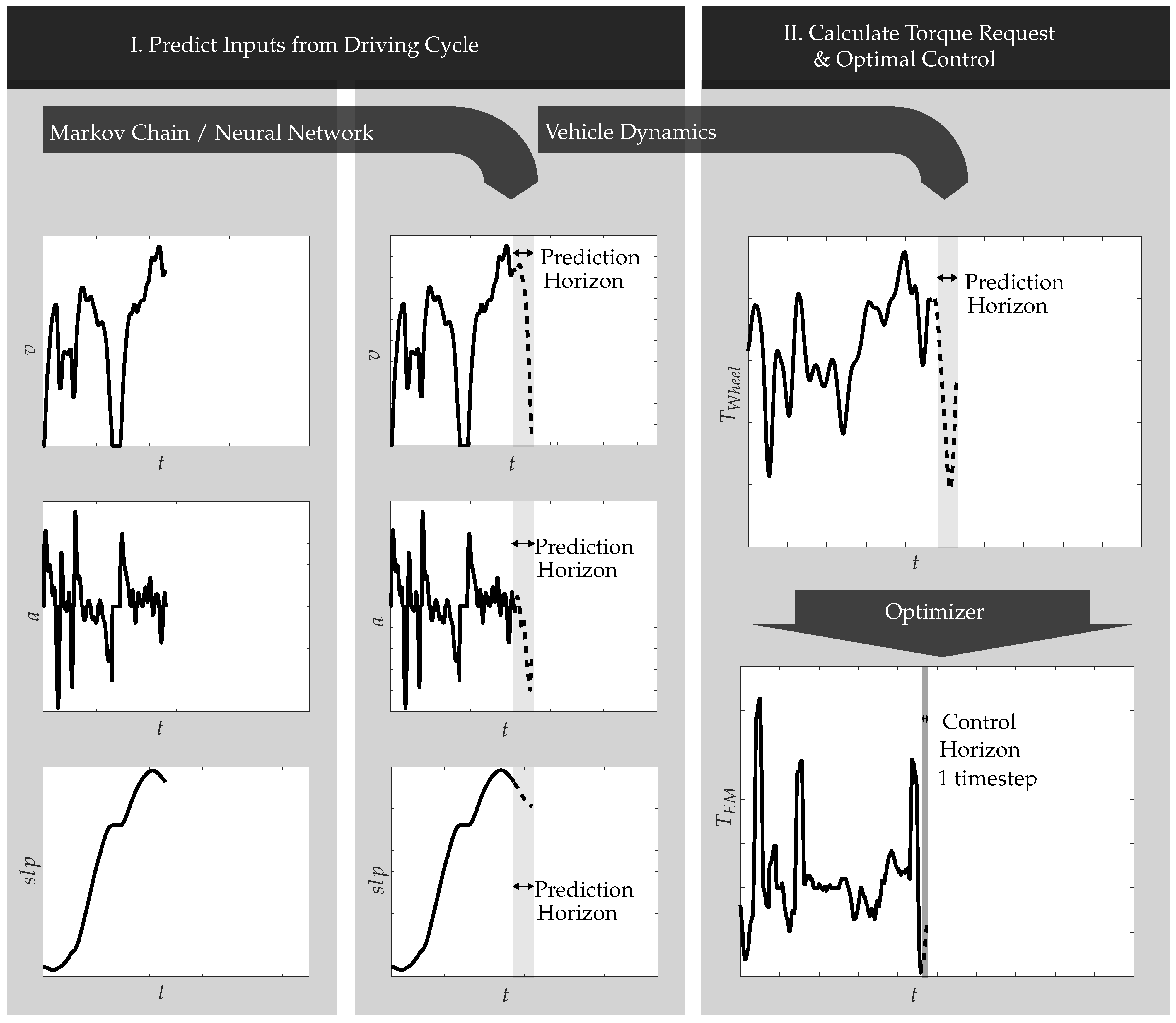
The basic Generic Model Predictive Control Scheme considered in this work is visualized in
Figure 1, whereby the driver behaviour is predicted for the route ahead based on the statistical model. Therefore, at first, all torque-relevant values like velocity, acceleration, and slope are predicted for a given horizon. In the next step, the expected torque request is calculated using a model of vehicle dynamics. Based on this information, finally, an optimal control value can be determined by the chosen optimizer.
As already stated, two different approaches from the field of stochastics as well as artificial intelligence for generating such predictions are considered in this work. Their basic characteristics are briefly described below.
3.2. Discrete Markov Processes
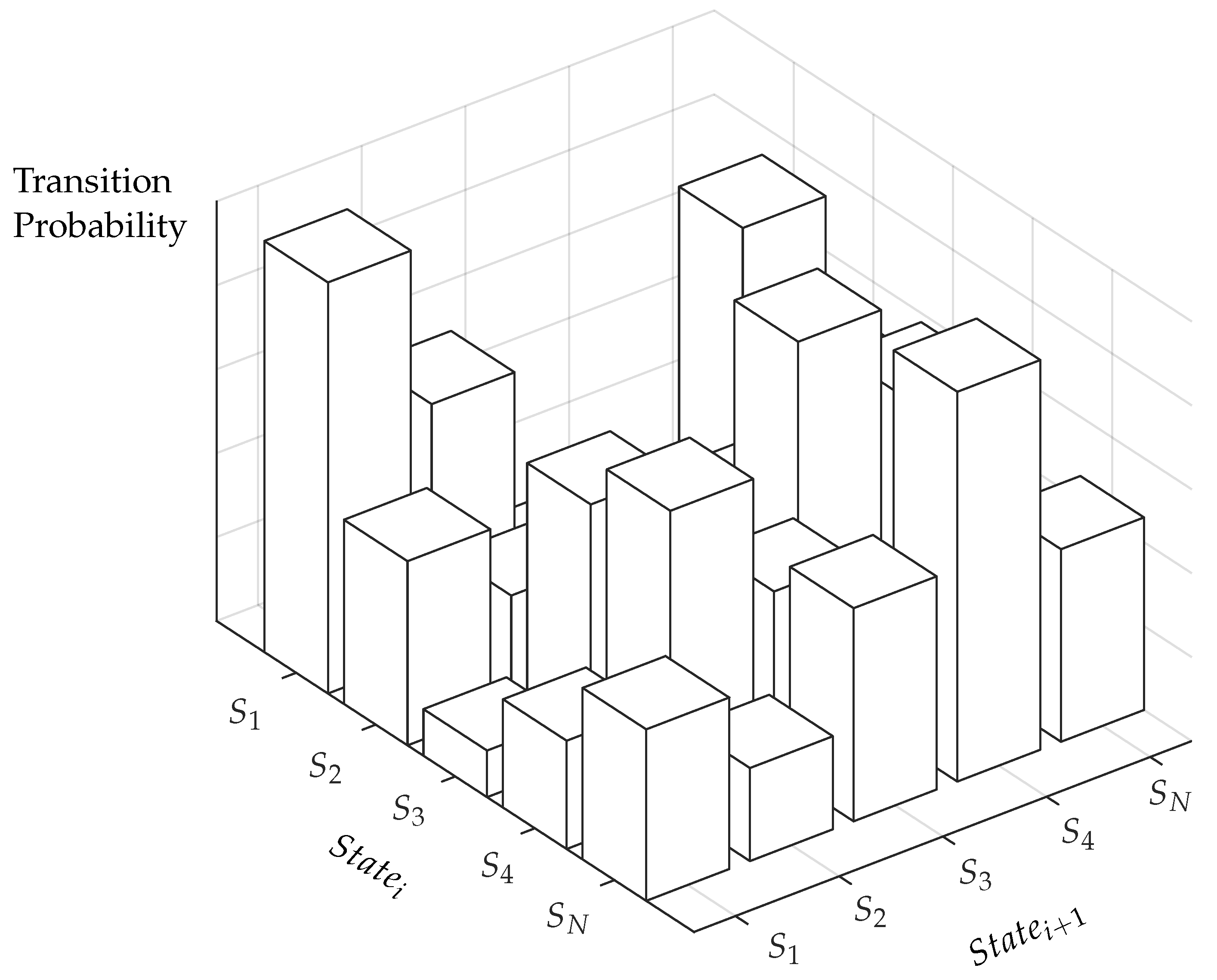
In discrete Markov processes, the states of a system are discretized, whereby the system state can be described at any time by one of these states. This allows the calculation of a transition probability which subsequent state occurs at a certain actual state. These transition probabilities in turn are stored in a Transition Probability Matrix (TPM), see
Figure 2.
If this probability distribution is limited to the current state without taking into account past values, this can be stated as a first-order MC. If we further denote the states as
S, the state at time
t as
, and the transition probability from state
i to state
j as
, the following applies [
44]:
Since only time-invariant processes are considered, the following results:
Furthermore, the following properties for the transition probability
apply:
3.3. Feedforward Neural Networks
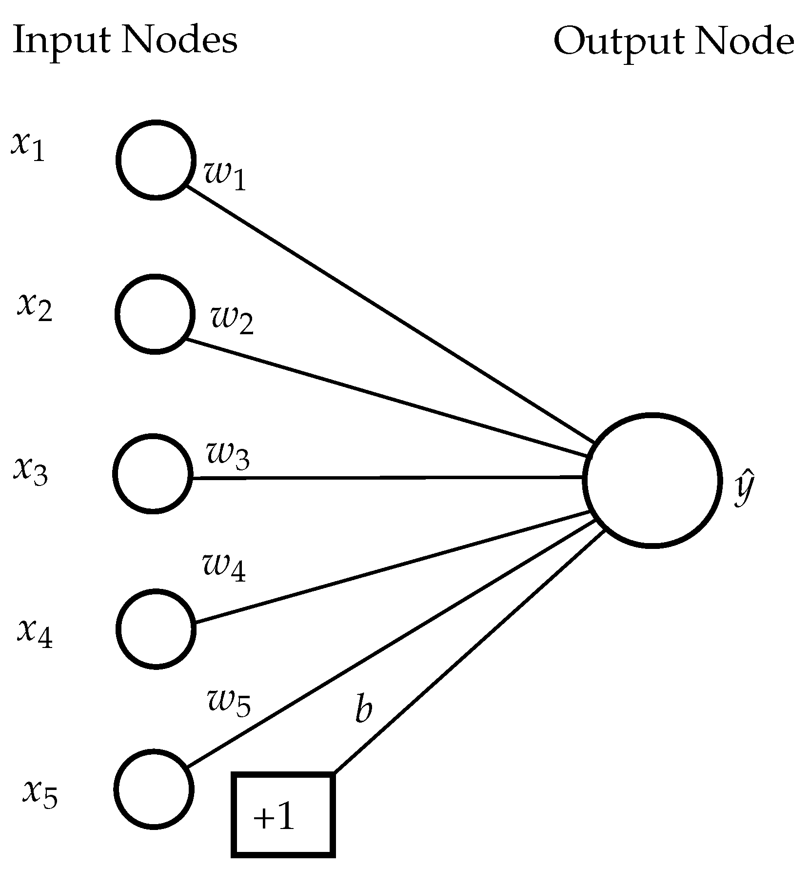
A Feedforward Neural Network (FNN) typically consists of an input layer, an output layer, and several hidden layers. The basic calculations will be shown in the example of a neural network with a single output neuron, the perceptron in
Figure 3.
The output value
is a result of taking into account the input variables
corresponding to the
d features, the bias
b, the weights of the connections between the input layer and the output neuron
, as well as the activation function
, according to the following relationship [
45]:
In this context, the activation function is applied to the weighted sum of the input values and thus finally determines the output value of the neuron. A typical activation function is, for example, the Rectified Linear Unit (ReLu), but other functions can also be used depending on the application [
45]. This basic principle can also be transferred to more complex neural networks. Here, the output values of one layer result in the input values for the neurons in the next layer. For a comprehensive overview of FNN including the various calibration possibilities, the reader is referred to [
45].
3.4. Procedure Overview
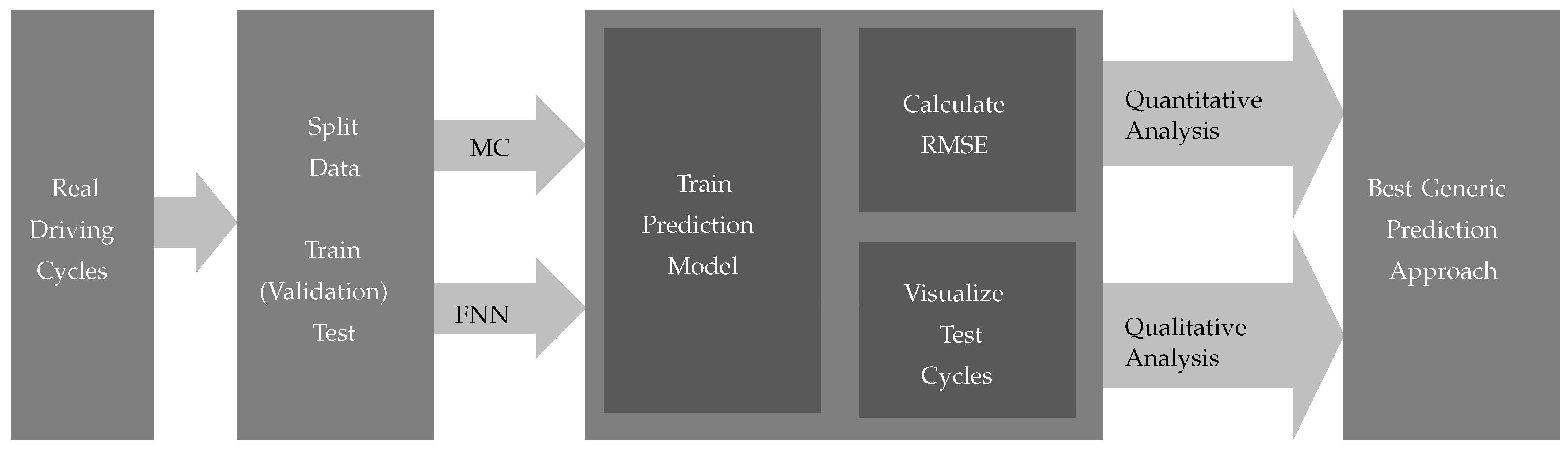
The basic procedure is shown in
Figure 4. Here, the real driving cycles further described in
Section 4.1 are first divided into training, validation, and test data in the ratio 60:20:20. Subsequently, models for MC and FNN are trained. Through a subsequent analysis of the calculated RMSE values of velocity, acceleration, and road slope as well as by analysing the predictions with corresponding plots of the whole driving cycle, the optimal generic prediction approach for the purpose described will be finally selected.
4. Implementation
4.1. Available Data
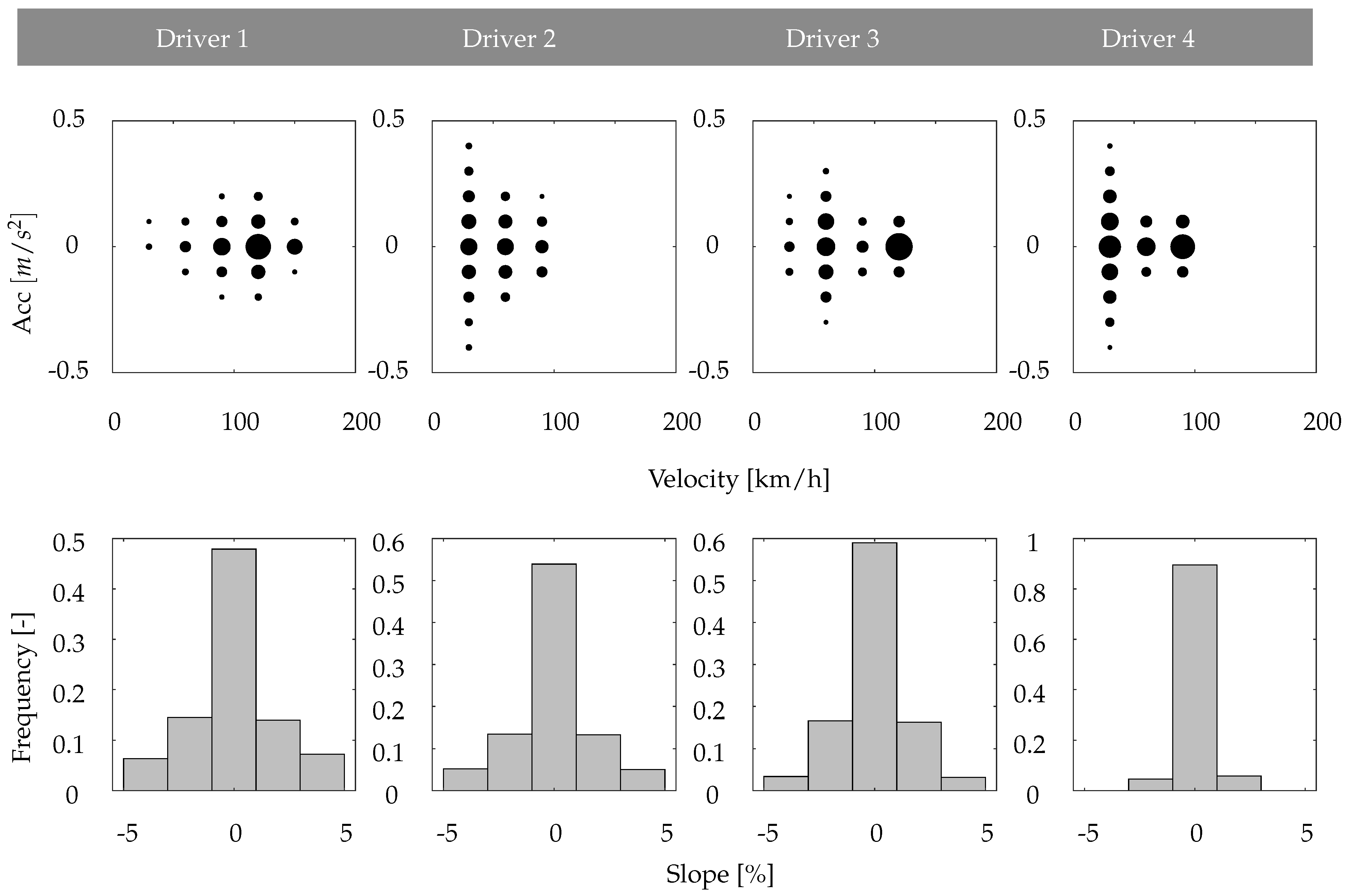
For the application of the presented methodology, driving data from a total of four test drivers are available. As shown in
Table 2, the four test drivers differ in major characteristic values. Basically, driver 1 has driven by far the most test kilometres and also has the longest total test time. Maximum velocities as well as maximum accelerations and decelerations achieved the highest values here. On average, however, relatively low accelerations occur as the lowest
(Root Mean Squared) value shows. This is also underlined by the v-a plot in
Figure 5.
It can be concluded that driver 1 drives mostly on the highway. Driver 2 is characterised by the highest proportion of standstill times and the highest average accelerations. As the v-a plot further shows, driver 2 primarily drives in urban areas and occasionally on country roads. As also shown in
Figure 5 the focus of driver 3 is on city driving or driving on the highway at a constant speed of 120 km/h. The rides of driver 4 also have a high proportion of low acceleration, especially on country roads in the 80–100 km/h velocity range. Regarding the driven road slopes, driver 4 has hardly any road slopes in the range of ±5%, while drivers 1–3 have a similar distribution.
4.2. Model Architectures
As introduced in
Section 3.2 discrete Markov processes states have to be defined. In accordance with [
13,
15] each state is represented by a 3 × 1 tuple consisting of vehicle velocity
, acceleration
, and road slope
:
If the slope is not taken into account, the state is reduced to a 2 × 1 tuple. The discretisation of the relevant quantities is worked out by extensive parameter studies, further described in
Section 4.3. In order to predict torque-relevant quantities using MC, first the TPM must be calculated from training data. Afterwards, a MC object is created using the
dtmc-function of the MATLAB Econometrics Toolbox. Now, the predictions can be computed by a random walk through the MC according to the prediction horizon.
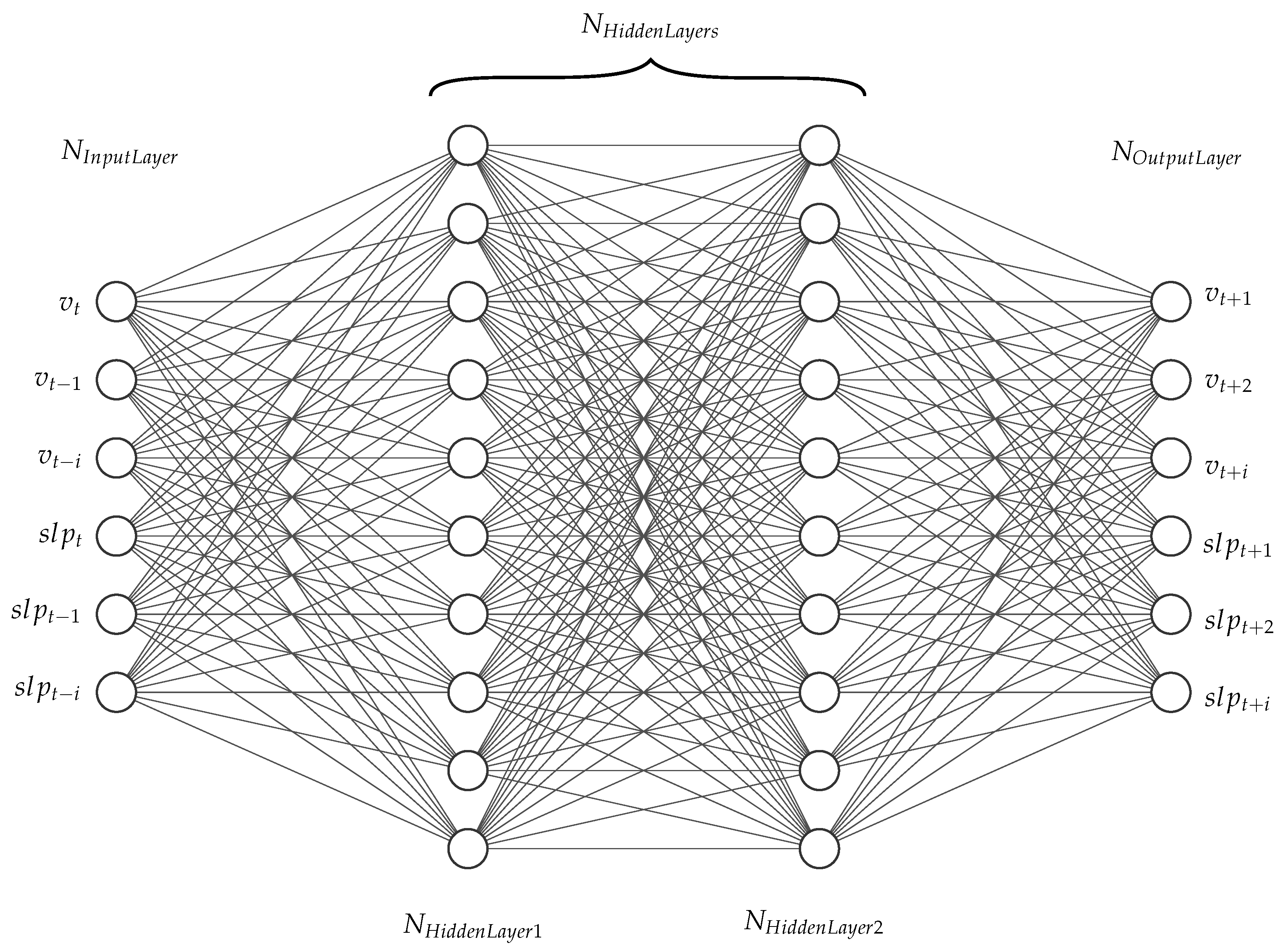
When modelling the FNN described in
Section 3.3 and shown in
Figure 6, the inputs and outputs are selected analogously to [
31]. In this source, the inputs represent the considered time horizon in the past, whereas the outputs represent the predicted time horizon in the future. The numbers of inputs and outputs are always chosen equally in this work, so a prediction horizon into the future of 20 s also requires a consideration of the last 20 s. If the road slope is taken into account, the number of inputs and outputs doubles accordingly. In contrast to the MC, explicit modelling of the accelerations is not performed. This is due to the fact that accelerations are already taken into account by the sequence of velocities indirectly.
The FNN is implemented in Python using Keras. Keras is a neural network library built on the TensorFlow platform. The number of hidden layers and their number of neurons, the loss function, the activation function, and other parameters are checked by extensive studies which are described in excerpts in the following section.
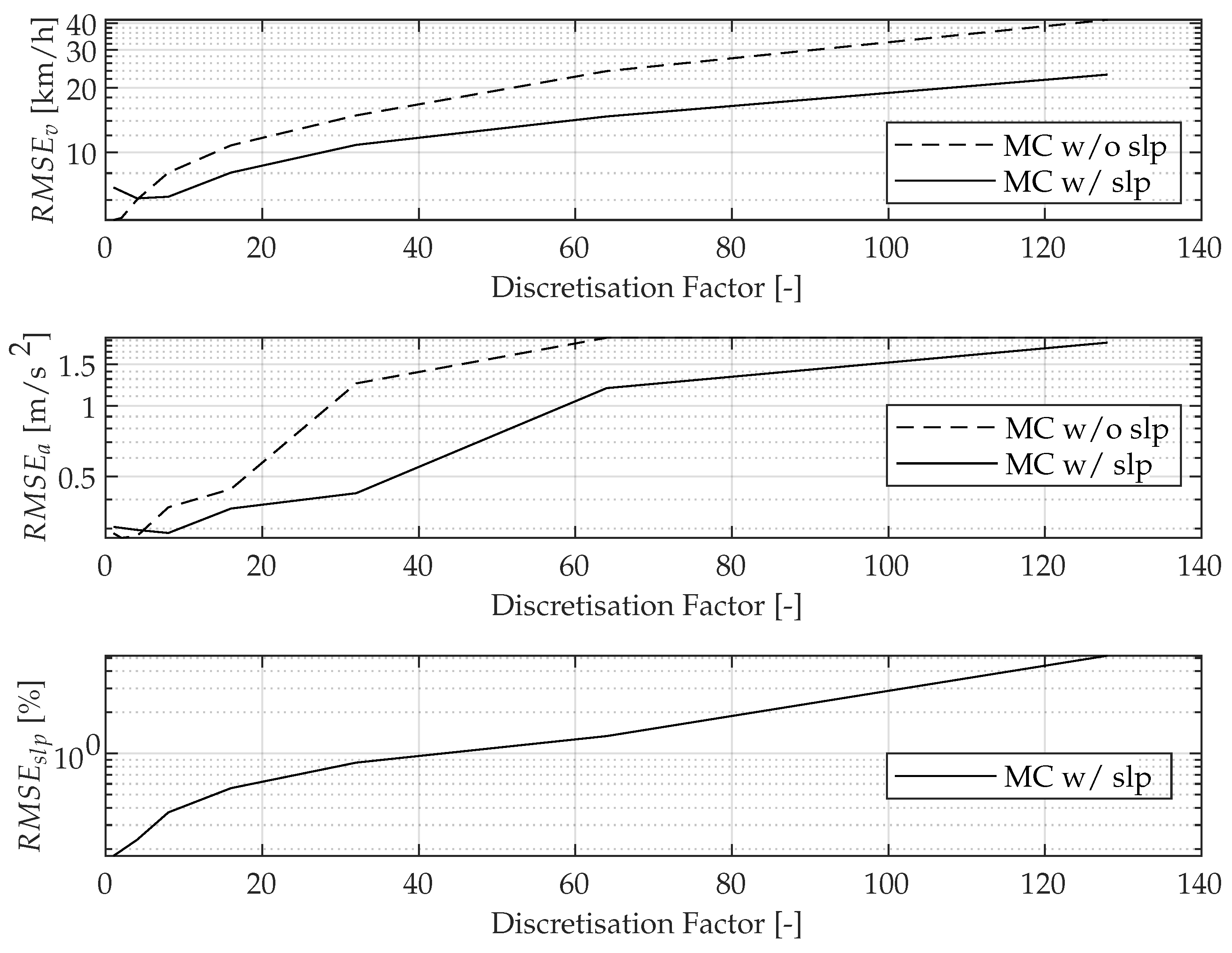
4.3. Parameter Studies
For the choice of a suitable discretisation, the discretisation is increased by a discretisation factor on the basis of the values in the literature [
13,
15]. The studies are shown in
Figure 7. Due to the convergence of velocity and acceleration, the proposed parametrisation of
Table 3 (discretisation factor of 1) can be confirmed as suitable. As can be seen, the
converges to ≈5 km/h, and the
converges to ≈0.3 m/s
for a prediction horizon of 10 s for the chosen test dataset.
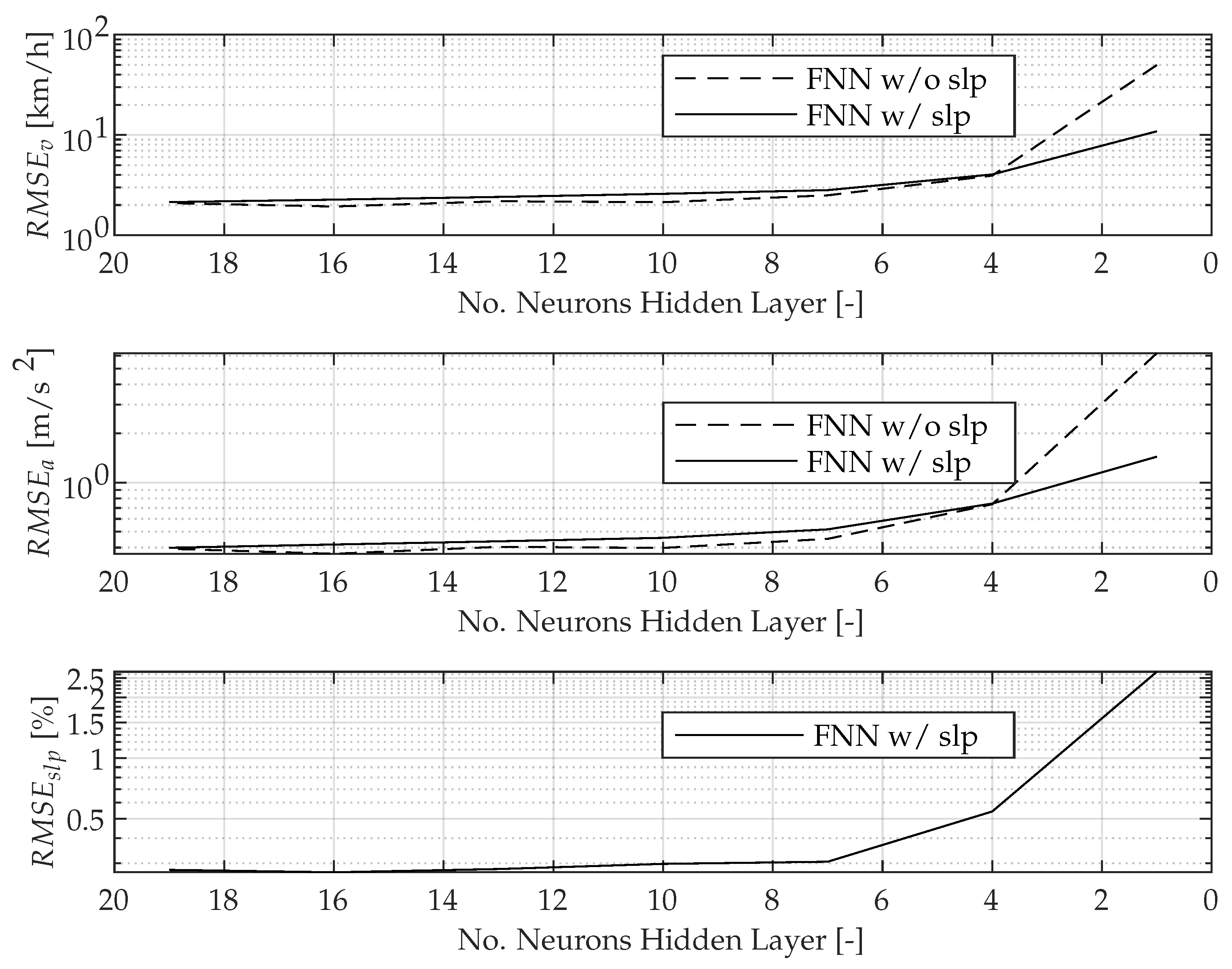
The same procedure is used to select the number of neurons for the hidden layers of the neural network. For the choice of a suitable number of neurons, the number of neurons in the hidden layers are reduced from values in the literature (
Figure 8). Due to the convergence of velocity and acceleration, the parametrisation proposed in
Table 4 (no. neurons hidden layer of 10) can be confirmed as suitable. As can be seen, the
converges to ≈2 km/h, and the
converges to ≈0.4 m/s
for a prediction horizon of 10 s for the chosen test dataset.
Further parameter analyses are not discussed at this point.
4.4. Final Model Parameters
In
Table 3 and
Table 4, the final parameters are shown for the MC and the FNN.
Using a Rectified Linear Unit (ReLu) Activation Function as well as the Mean Squared Error (MSE) as a Loss function leads to the best results. The amount of hidden layers and their amount of neurons as well as the other parameters listed were developed through corresponding parameter studies. Parameters not listed in
Table 4 were left at default settings of
Keras.
5. Results
5.1. Evaluation of the Root Mean Squared Error (RMSE)
Table 5 shows that prediction accuracies using MC are similar for all drivers. As an example, for a prediction horizon of 10 s, the
is about 4 km/h. Only
of driver 2 with a high standstill percentage and the highest accelerations is slightly higher with an
of 4.62 km/h. Taking the road slope into account cannot increase the prediction accuracy any further. However apart from driver 4, where the value remains almost constant, all drivers even show a deterioration of a few percent when considering road slope. In addition, an overproportional increase in the RMSE values can be seen when the prediction horizon is increased to 20 s or 30 s. This suggests that MC are particularly unsuitable for large prediction horizons.
As shown in
Table 6 for all four drivers, the application of the FNN leads to a higher prediction accuracy in total. The RMSE of the calculated velocities is 30% less compared to the results of MC. Especially the avoidance of an overproportional increase for a prediction horizon of 20 s or 30 s should be mentioned at this point. Apart from that, in contrast to MC, the FNN seems to best match the driving style of driver 4. Also, for FNN, the RMSE values for the accelerations are higher than for the MC. The authors justify this by the fact that, in contrast to the MC, the accelerations were only indirectly taken into account in the FNN and therefore merely
is minimized during training. Furthermore, there is a clear improvement in the prediction accuracy of the slope. Besides, a significantly lower deterioration in velocity and acceleration accuracy can be seen when using road slope overall. However, an improvement by taking into account road slope (e.g., slope leads to velocity increase) is not detected here either.
5.2. Evaluation of Predictions in Time Domain
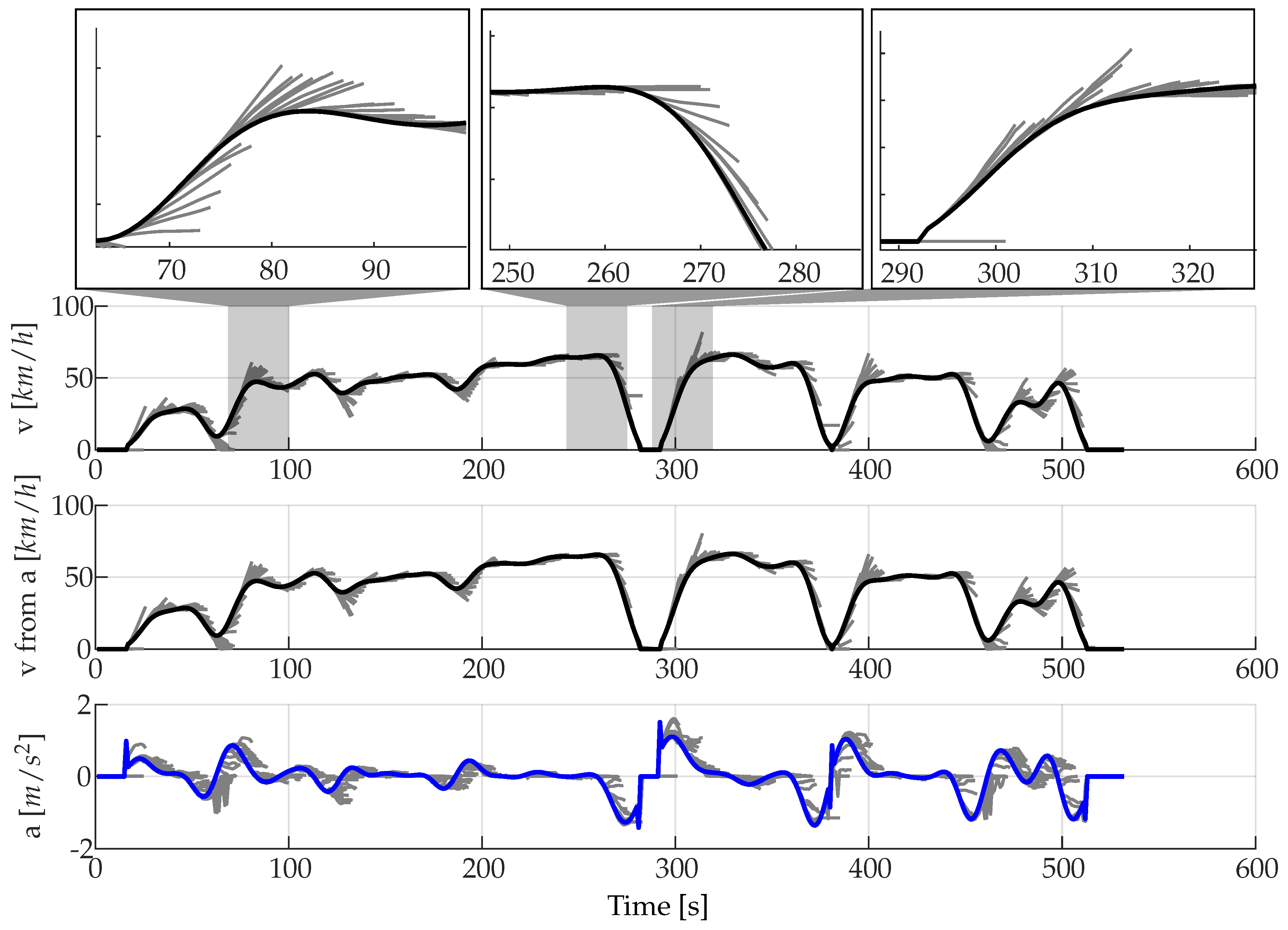
As shown in
Figure 9, MC allow both a velocity and acceleration curve to be predicted, whereby the resulting velocity curve from the integrated acceleration has a slightly lower RMSE. Therefore, only velocities from the integrated acceleration signal are compared with actual velocity values in
Table 5. The decisive factor here is how individual states in the real driving cycle, that are not included in the training cycles, are treated. In this work, the assumption of remaining in the current state is chosen. Thus, the constant acceleration provides better values than the assumption of a constant velocity due to the fact that the resulting velocity of constant acceleration is more realistic. This behaviour can be seen at t = 280 s and t = 380 s. Generally, the MC show best prediction accuracy in areas of low dynamics. In the case of an acceleration manoeuvre, however, such as occurs at t = 80 s, the transition to relatively constant velocity is only predicted correctly when the maximum velocity has almost been reached. Similar results can be seen during deceleration at t = 260 s, which is only correctly recognised after the braking process has started. Also, the starting process could only be predicted after the rise of speed (t = 290 s). Until this happens, a velocity of zero is predicted. However, constant velocity phases are always predicted from the MC properly. The MC deliver plausible results overall and prove to be suitable for the prediction of the velocity and acceleration.
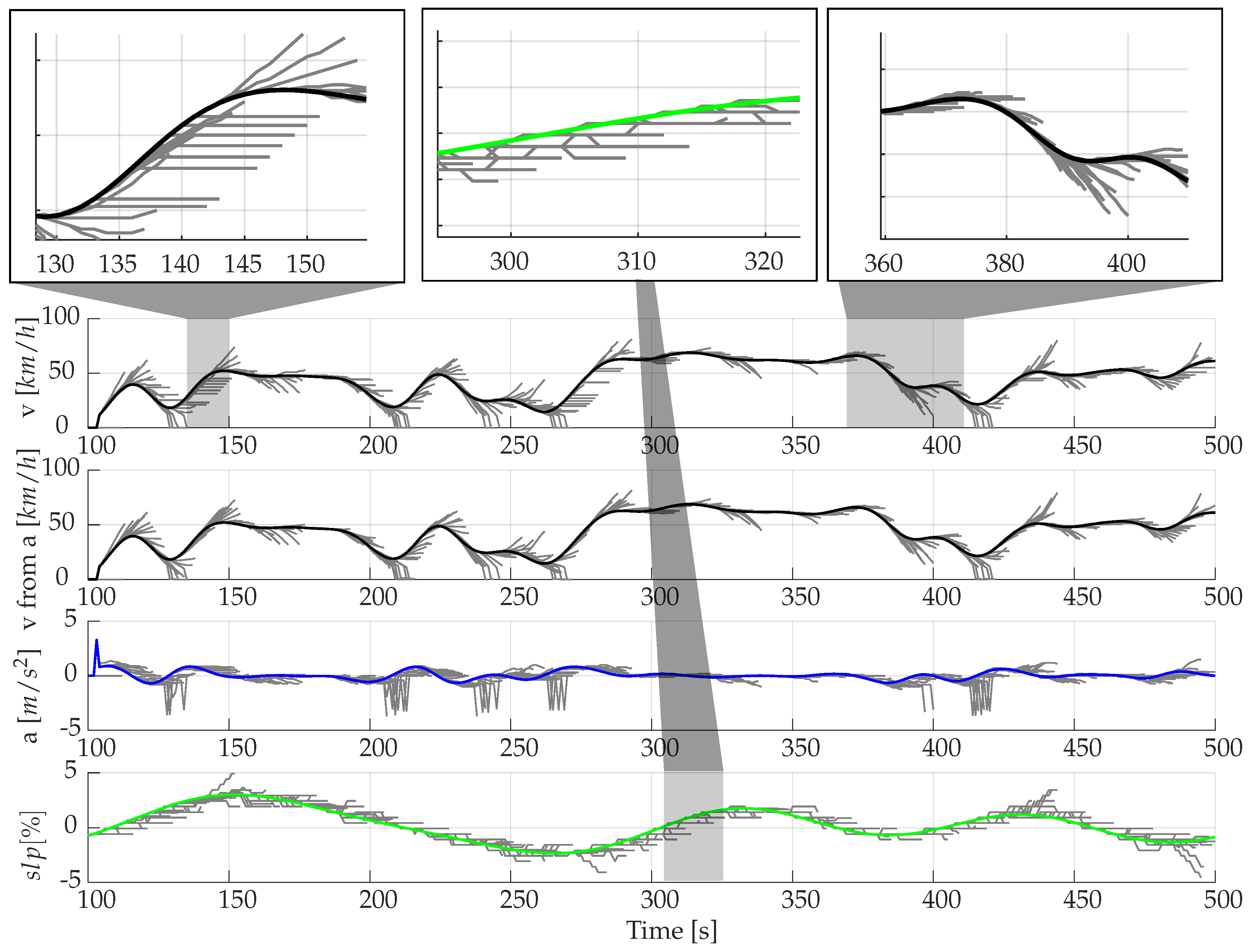
The performance of MC when taking the slope into account can be well illustrated by the example shown below (
Figure 10). In principle, the performance is similar to that of MC which are only velocity—and acceleration-based (
Figure 9). However, since an individual state is now additionally characterised by the road slope, there tend to be more driving states that cannot be directly assigned to a Markov state (see t = 140 s). In these cases, the current state is kept constant as described previously. Also, in individual cases, unrealistic predictions can be recognised. This can be seen at t = 170 s, where even a constant velocity section cannot be adequately predicted. Although an assignment is possible here, the statistical features from the velocity, acceleration, and geographical profile are not sufficiently stored in the MC. A coarser discretisation can lead to better results in these individual cases, since more states can be assigned to the same state. However, this results in poorer predictions overall, as is also clearly evident from
Figure 7.
Furthermore, it can be seen in the last plot of
Figure 10 that both the actual and subsequent state are often assigned to the same state for the road slope. This means that apart from the assignment to a state in the first timestep of the prediction, the probability of a change of state is very low in the slope profile. If a state change nevertheless occurs, the choice of the next state of the slope appears arbitrary and does not follow the current trend of the slope. The information obtained from the combination with current velocity and acceleration thus seems to be insufficient for an adequate prediction of the slope profile.
An improvement of the prediction quality with regard to velocity and acceleration by taking into account the interactions with the road slopes that occurred in the MC cannot be determined neither in the plot nor in the calculated RMSE values. Lastly, the derivative of the slope is introduced as an additional feature of a state, analogous to velocity and acceleration in order to better identify trends in the road slope. However, since a state of the MC is defined by a total of four parameters in this case, an additional challenge arises from the increased computational effort in order to sufficiently train all states of the MC. Accordingly this approach is not further discussed.
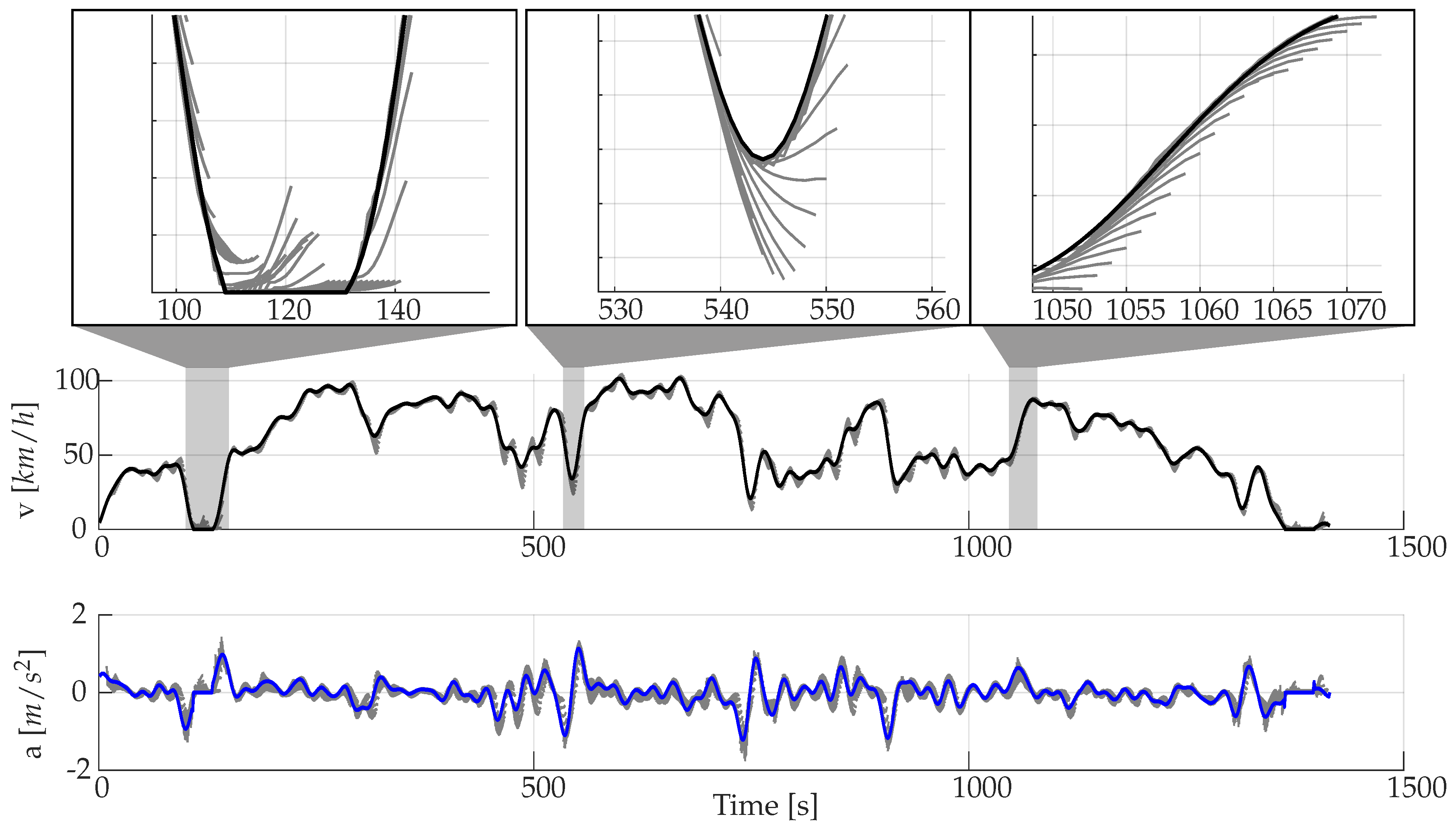
The FNN basically shows a similar performance in the analysis of the predictions in the time domain as the MC (
Figure 11). Similarly, acceleration or deceleration phases are predicted only when they are already initiated (t = 530 s), whereby the individual predictions can differ: While the MC tends to expect a higher velocity increase in
Figure 9 at t = 310 s than occurs actually, the FNN in
Figure 11 assumes a lower velocity increase in a comparable driving phase at t = 1050 s. Similarly, in
Figure 9 at t = 290 s, as already mentioned, a further standstill is expected, while the FNN in a similar situation in
Figure 11 at t = 120 s always wants to accelerate. The latter example shows very clearly the fundamentally different mode of operation. In the case of standstill, the most probable subsequent state is a further standstill (the start-up process only occurs at a single timestep) and the TPM of the MC is trained accordingly. However, in the FNN, no bins were filled with transitions that actually occurred, but the network was merely trained for the lowest MSE overall.
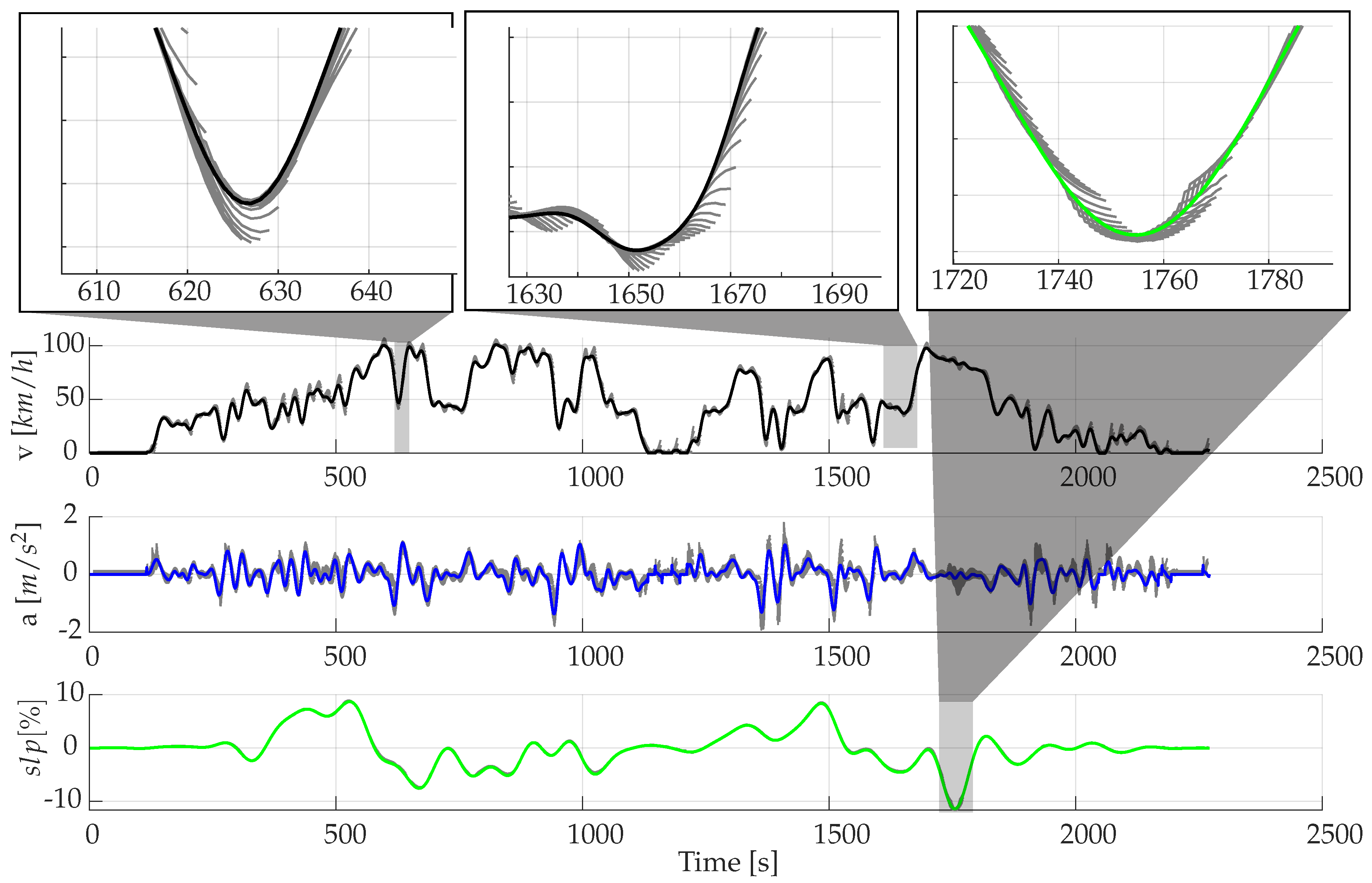
As shown in
Figure 12, the performance of predicting velocity and acceleration is almost similar to the predictions shown in
Figure 11. However, slopes can be predicted much better here than with the use of MC. Also, in contrast to the MC, the introduction of the slope leads to hardly any deterioration of the predictions. This results from the fact that in contrast to MC, also unknown conditions can be dealt with properly. The small differences between the predicted and real velocity profiles result in the already presented low RMSE values from
Table 6.
6. Conclusions
In order to apply predictive driving strategies, a robust prediction approach is necessary. However, most prediction approaches need additional data to provide predictions, whereby a continuous availability of these data cannot be ensured any time. Within the scope of this work, therefore, two intelligent methods were identified. Here, for the predictions, only the current and past driving conditions are required. To train the model, only historical driving data are needed.
First of all, it could be shown that the driving style and also the driven slopes of the real drivers’ rides differ significantly from each other. This allowed a wide range of potential driving characteristics to be investigated. Subsequently, two approaches from the field of stochastics and artificial intelligence were applied to the driving profiles and evaluated with regard to their predictive quality. After calibrating the models appropriately, both quantitative analyses regarding RMSE values and qualitative analyses in the time domain were performed for each approach.
Regarding the qualitative analysis, the predictions of MC and FNN seem to perform relatively similarly at first glance for a prediction horizon of 10 s. However, there are individual advantages and disadvantages in the respective prediction which can be explained by fundamental differences in the model architectures. Further analysis in time domain showed that MC as well as FNN can predict trends only to a limited extent. Thus, it can be generally stated that dynamic changes in the driven profile can only be recognised when they have already been initiated.
From the quantitative analyses, it could be shown that FNN can actually achieve ≈30% more accurate velocity predictions and lead to higher accuracy in total compared to MC, especially when road slope is taken into account. Furthermore, MC show an overproportional increase at larger prediction horizons in contrast to FNN. However, an improvement in the prediction quality by considering road slope cannot be determined neither for MC nor for FNN.
To summarize, FNN should be preferred to MC. Further work should deal with how a FNN can be enriched with additional information to make the predictions more precise. If available, the simple extensibility of the FNN enables the use of Radar, Lidar, and camera or environment data from C2C, C2X, as well as navigation systems to predict dynamics before they occur. In this way, the individual driving strategy can get closer to the global optimum. Furthermore, this enables the opportunity to perform long-term predictions in order to provide additional information to the driving strategy.
Author Contributions
Conceptualization, F.D.; methodology, F.D.; software, F.D.; validation, F.D., formal analysis, F.D.; investigation, F.D.; resources, F.D.; data curation, F.D.; writing—original draft preparation, F.D.; writing—review and editing, F.D.; visualization, F.D.; supervision, M.G. and F.G. All authors have read and agreed to the published version of the manuscript.
Funding
This research was funded by Mercedes-Benz AG.
Institutional Review Board Statement
Not applicable.
Informed Consent Statement
Not applicable.
Data Availability Statement
Not applicable.
Acknowledgments
The authors would like to thank Mercedes-Benz AG for funding this project. We acknowledge support by the KIT-Publication Fund of the Karlsruhe Institute of Technology.
Conflicts of Interest
The authors declare no conflict of interest.
References
- Silvas, E.; Hofman, T.; Murgovski, N.; Etman, P.; Steinbuch, M. Review of Optimization Strategies for System-Level Design in Hybrid Electric Vehicles. IEEE Trans. Veh. Technol. 2016, 66, 57–70. [Google Scholar] [CrossRef]
- Tran, D.D.; Vafaeipour, M.; El Baghdadi, M.; Barrero, R.; van Mierlo, J.; Hegazy, O. Thorough state-of-the-art analysis of electric and hybrid vehicle powertrains: Topologies and integrated energy management strategies. Renew. Sustain. Energy Rev. 2020, 119, 109596. [Google Scholar] [CrossRef]
- Serrao, L. A Comparative Analysis Of Energy Management Strategies For Hybrid Electric Vehicles. Ph.D. Thesis, Ohio State University, Columbus, OH, USA, 2009. [Google Scholar]
- Rizzoni, G.; Onori, S. Energy Management of Hybrid Electric Vehicles: 15 years of development at the Ohio State University. Oil Gas Sci. Technol./Rev. D’Ifp Energies Nouv. 2015, 70, 41–54. [Google Scholar] [CrossRef] [Green Version]
- Xu, N.; Kong, Y.; Chu, L.; Ju, H.; Yang, Z.; Xu, Z.; Xu, Z. Towards a Smarter Energy Management System for Hybrid Vehicles: A Comprehensive Review of Control Strategies. Appl. Sci. 2019, 9, 2026. [Google Scholar] [CrossRef] [Green Version]
- Jiang, Q.; Ossart, F.; Marchand, C. Comparative Study of Real-Time HEV Energy Management Strategies. IEEE Trans. Veh. Technol. 2017, 66, 10875–10888. [Google Scholar] [CrossRef] [Green Version]
- Joševski, M. Predictive Energy Management of Hybrid Electric Vehicles with Uncertain Torque Demand Forecast for On-Road Operation. Ph.D. Thesis, Rheinisch-Westfälische Technische Hochschule Aachen University, Aachen, Germany, 2017. [Google Scholar]
- Huang, Y.; Wang, H.; Khajepour, A.; He, H.; Ji, J. Model predictive control power management strategies for HEVs: A review. J. Power Sources 2017, 341, 91–106. [Google Scholar] [CrossRef]
- Zhou, Q.; Du, C. A quantitative analysis of model predictive control as energy management strategy for hybrid electric vehicles: A review. Energy Rep. 2021, 7, 6733–6755. [Google Scholar] [CrossRef]
- Lee, T.K.; Filipi, Z.S. Synthesis and validation of representative real-world driving cycles for Plug-In Hybrid vehicles. In Proceedings of the 2010 IEEE Vehicle Power and Propulsion Conference, Lille, France, 1–3 September 2010; pp. 1–6. [Google Scholar] [CrossRef]
- Lee, T.K.; Adornato, B.; Filipi, Z.S. Synthesis of real-world driving cycles and their use for estimating PHEV energy consumption and charging opportunities: Case study for Midwest/U.S. IEEE Trans. Veh. Technol. 2011, 60, 4153–4163. [Google Scholar] [CrossRef]
- Nyberg, P.; Frisk, E.; Nielsen, L. Using real-world driving databases to generate driving cycles with equivalence properties. IEEE Trans. Veh. Technol. 2016, 65, 4095–4105. [Google Scholar] [CrossRef]
- Silvas, E.; Hereijgers, K.; Peng, H.; Hofman, T.; Steinbuch, M. Synthesis of Realistic Driving Cycles With High Accuracy and Computational Speed, Including Slope Information. IEEE Trans. Veh. Technol. 2016, 65, 4118–4128. [Google Scholar] [CrossRef]
- Liessner, R.; Dietermann, A.M.; Bäker, B.; Lüpkes, K. Derivation of real-world driving cycles corresponding to traffic situation and driving style on the basis of Markov models and cluster analyses. In Proceedings of the 6th Hybrid and Electric Vehicles Conference (HEVC 2016), London, UK, 2–3 November 2016. [Google Scholar]
- Forster, D.; Inderka, R.B.; Gauterin, F. Data-Driven Identification of Characteristic Real-Driving Cycles Based on k-Means Clustering and Mixed-Integer Optimization. IEEE Trans. Veh. Technol. 2020, 69, 2398–2410. [Google Scholar] [CrossRef]
- Zähringer, M.; Kalt, S.; Lienkamp, M. Compressed Driving Cycles Using Markov Chains for Vehicle Powertrain Design. World Electr. Veh. J. 2020, 11, 52. [Google Scholar] [CrossRef]
- Bichi, M.; Ripaccioli, G.; Di Cairano, S.; Bernardini, D.; Bemporad, A.; Kolmanovsky, I.V. Stochastic model predictive control with driver behavior learning for improved powertrain control. In Proceedings of the 49th IEEE Conference on Decision and Control (CDC), Atlanta, GA, USA, 15–17 December 2010; pp. 6077–6082. [Google Scholar] [CrossRef]
- Di Cairano, S.; Bernardini, D.; Bemporad, A.; Kolmanovsky, I.V. Stochastic MPC With Learning for Driver-Predictive Vehicle Control and its Application to HEV Energy Management. IEEE Trans. Control. Syst. Technol. 2014, 22, 1018–1031. [Google Scholar] [CrossRef]
- Josevski, M.; Abel, D. Energy Management of Parallel Hybrid Electric Vehicles based on Stochastic Model Predictive Control. IFAC Proc. Vol. 2014, 17, 2132–2137. [Google Scholar] [CrossRef] [Green Version]
- Zeng, X.; Wang, J. A Parallel Hybrid Electric Vehicle Energy Management Strategy Using Stochastic Model Predictive Control With Road Grade Preview. IEEE Trans. Control. Syst. Technol. 2015, 23, 2416–2423. [Google Scholar] [CrossRef]
- Li, L.; You, S.; Yang, C.; Yan, B.; Song, J.; Chen, Z. Driving-behavior-aware stochastic model predictive control for plug-in hybrid electric buses. Appl. Energy 2016, 162, 868–879. [Google Scholar] [CrossRef]
- Vadamalu, R.S.; Beidl, C. Explicit MPC PHEV energy management using Markov chain based predictor: Development and validation at Engine-In-The-Loop testbed. In Proceedings of the 2016 European Control Conference (ECC), Aalborg, Denmark, 29 June–1 July 2016; pp. 453–458. [Google Scholar] [CrossRef]
- Qin, F.; Xu, G.; Hu, Y.; Xu, K.; Li, W. Stochastic Optimal Control of Parallel Hybrid Electric Vehicles. Energies 2017, 10, 214. [Google Scholar] [CrossRef]
- Xie, S.; He, H.; Peng, J. An energy management strategy based on stochastic model predictive control for plug-in hybrid electric buses. Appl. Energy 2017, 196, 279–288. [Google Scholar] [CrossRef]
- Xie, S.; Hu, X.; Xin, Z.; Brighton, J. Pontryagin’s Minimum Principle based model predictive control of energy management for a plug-in hybrid electric bus. Appl. Energy 2019, 236, 893–905. [Google Scholar] [CrossRef] [Green Version]
- Zhao, B.; Lv, C.; Hofman, T. Driving-Cycle-Aware Energy Management of Hybrid Electric Vehicles Using a Three-Dimensional Markov Chain Model. Automot. Innov. 2019, 2, 146–156. [Google Scholar] [CrossRef]
- Yang, C.; You, S.; Wang, W.; Li, L.; Xiang, C. A Stochastic Predictive Energy Management Strategy for Plug-in Hybrid Electric Vehicles Based on Fast Rolling Optimization. IEEE Trans. Ind. Electron. 2020, 67, 9659–9670. [Google Scholar] [CrossRef]
- Sun, C.; Hu, X.; Moura, S.J.; Sun, F. Comparison of velocity forecasting strategies for predictive control in HEVs. In Proceedings of the ASME 2014 Dynamic Systems and Control Conference, San Antonio, TX, USA, 22–24 October 2014. [Google Scholar]
- Sun, C.; Hu, X.; Moura, S.J.; Sun, F. Velocity Predictors for Predictive Energy Management in Hybrid Electric Vehicles. IEEE Trans. Control. Syst. Technol. 2015, 23, 1197–1204. [Google Scholar] [CrossRef]
- Sun, C.; Sun, F.; He, H. Investigating adaptive-ECMS with velocity forecast ability for hybrid electric vehicles. Appl. Energy 2017, 185, 1644–1653. [Google Scholar] [CrossRef]
- Xie, S.; Hu, X.; Xin, Z.; Li, L. Time-Efficient Stochastic Model Predictive Energy Management for a Plug-In Hybrid Electric Bus With an Adaptive Reference State-of-Charge Advisory. IEEE Trans. Veh. Technol. 2018, 67, 5671–5682. [Google Scholar] [CrossRef]
- Liu, H.; Li, X.; Wang, W.; Han, L.; Xiang, C. Markov velocity predictor and radial basis function neural network-based real-time energy management strategy for plug-in hybrid electric vehicles. Energy 2018, 152, 427–444. [Google Scholar] [CrossRef]
- Xiang, C.; Ding, F.; Wang, W.; He, W. Energy management of a dual-mode power-split hybrid electric vehicle based on velocity prediction and nonlinear model predictive control. Appl. Energy 2017, 189, 640–653. [Google Scholar] [CrossRef]
- Xie, S.; Hu, X.; Qi, S.; Lang, K. An artificial neural network-enhanced energy management strategy for plug-in hybrid electric vehicles. Energy 2018, 163, 837–848. [Google Scholar] [CrossRef] [Green Version]
- Lin, X.; Wang, Z.; Wu, J. Energy management strategy based on velocity prediction using back propagation neural network for a plug–in fuel cell electric vehicle. Int. J. Energy Res. 2021, 45, 2629–2643. [Google Scholar] [CrossRef]
- Xia, J.; Wang, F.; Xu, X. A Predictive Energy Management Strategy for Multi-mode Plug-in Hybrid Electric Vehicle based on Long short-term Memory Neural Network. IFAC PapersOnLine 2021, 54, 132–137. [Google Scholar] [CrossRef]
- Foerster, D.; Decker, L.; Doppelbauer, M.; Gauterin, F. Analysis of CO2 reduction potentials and component load collectives of 48 V-hybrids under real-driving conditions. Automot. Engine Technol. 2021, 6, 45–62. [Google Scholar] [CrossRef]
- Onori, S.; Serrao, L.; Rizzoni, G. Hybrid Electric Vehicles; Springer: London, UK, 2016. [Google Scholar] [CrossRef]
- Wahl, H.G. Optimale Regelung eines Prädiktiven Energiemanagements von Hybridfahrzeugen; KIT Scienfici Publishing: Karlsruhe, Germany, 2015. [Google Scholar]
- Guzzella, L.; Sciarretta, A. Vehicle Propulsion Systems: Introduction to Modeling and Optimization, 2nd ed.; Springer: Berlin, Germany; New York, NY, USA, 2007. [Google Scholar]
- Sun, C.; He, H.; Sun, F. The Role of Velocity Forecasting in Adaptive-ECMS for Hybrid Electric Vehicles. Energy Procedia 2015, 75, 1907–1912. [Google Scholar] [CrossRef] [Green Version]
- Back, M. Prädiktive Antriebsregelung zum Energieoptimalen Betrieb von Hybridfahrzeugen. Ph.D. Thesis, Karlsruhe University, Karlsruhe, Germany, 2005. [Google Scholar]
- Bauer, K.L. Echtzeit-Strategieplanung für Vorausschauendes Automatisiertes Fahren; KIT Scienfici Publishing: Karlsruhe, Germany, 2019. [Google Scholar]
- Rabiner, L.R. A tutorial on hidden Markov models and selected applications in speech recognition. Proc. IEEE 1989, 77, 257–286. [Google Scholar] [CrossRef] [Green Version]
- Aggarwal, C.C. Neural Networks and Deep Learning; Springer: Cham, Switzerland, 2018. [Google Scholar] [CrossRef]
| Publisher’s Note: MDPI stays neutral with regard to jurisdictional claims in published maps and institutional affiliations. |
© 2022 by the authors. Licensee MDPI, Basel, Switzerland. This article is an open access article distributed under the terms and conditions of the Creative Commons Attribution (CC BY) license (https://creativecommons.org/licenses/by/4.0/).


