Determination of Speed-Dependent Roadway Luminance for an Adequate Feeling of Safety at Nighttime Driving

Abstract

The purpose of this work is to determine as a function of velocity the minimal roadway luminance that is required to be judged as being bright enough for a driver to perform a nighttime driving task with an adequate feeling of safety. In this context, it shall also be evaluated which areas of the vehicle forefield are most crucial for the driver’s general brightness perception. A field study with 23 subjects and dimmable LED headlights was conducted, in which the subjects were given the task to assess their perceived brightness for different luminance levels caused by the headlights’ low-beam distribution in the vehicle’s forefield on a 5-step rating scale. The experiments were repeated for three different driving velocities of 0 km h⁻¹ (static case), 30 km h⁻¹, and 60 km h⁻¹, respectively. Results for the static case indicate that, for the roadway to be perceived as bright enough by 50% of the subjects, an average roadway luminance of 0.88 cd m⁻² is required in an area up to 32 m in front of the vehicle. Furthermore, a significant effect of driving speed is observed. For example, at 60 km h⁻¹, the luminance must be increased to 1.54 cd m⁻² to be still perceived as sufficiently bright by 50% of the subjects.

1. Introduction

The visual system is the driver’s primary source of information in road traffic [1,2,3,4]. It is responsible for recognizing and processing important information and dangers at an early stage. To guarantee a reliable and accurate visual system performance, adequate road lighting is required during both day- and nighttime driving. Providing sufficiently good lighting conditions at night is particularly important, as for example, in Germany, about 32% of all fatal accidents occur at dusk or in the dark hours [5], when visual capabilities are naturally reduced.

Various studies have shown that an increase in roadway luminance results in a significant decrease in nighttime accidents [6,7,8,9,10,11]. In addition, the driver’s subjective feeling of safety is also positively influenced [12,13,14,15]. Changes in roadway luminance thus show a significant impact on the safety of driving a motor vehicle in nighttime traffic. Objective parameters, such as accident statistics, and the more subjective perception of safety, are equally affected.

Empirical evidence for the impact of ambient and roadway luminance on the objective parameters of nighttime driving can be obtained by looking at accident statistics and research results for contrast perception and gaze behavior. Even though only about 20% of the daily traffic volume is observed during dark hours, more than one third of fatal accidents in Germany, and also in the European Union, occur at low ambient light conditions [16,17,18]. A study of accident trends in the period around the daylight saving time change (switch between summer and standard time) of Sullivan and Flannagan [7] confirms the high relevance of lighting conditions in the occurrence of traffic accidents. The results of their analysis showed that the time change and, thus, the associated sudden change in lighting conditions during the same morning and evening hours resulted in a considerable variation in accident numbers: They were able to show that, compared to driving in daylight, the probability of accidents involving pedestrians is by a factor of 3 to 6.75 higher after dark due to poorer visibility conditions. Similar results were reported by Plainis et al. [19], who examined accident statistics from Great Britain and Greece regarding injury severity in relation to the presence of street lighting systems. It was found that the presence of street lighting and the associated higher light levels of adaptation reduce injury severity by a factor of about 3. By analyzing Dutch accident statistics between 1987 and 2006, Wanvik [20] confirmed the positive influence of street and road lighting on the occurrence of accidents. In particular, they stated that proper nighttime illumination of streets and roadways is capable of reducing accidents with injuries by about 50%. According to Scott [6], who investigated the relationship between road lighting and accident frequency in built-up areas in Great Britain, the night/day accident ratio shows a high correlation with the mean roadway luminance in the range from 0.5 to 2 cd m⁻². They found that an increase in mean roadway luminance by 1 cd m⁻² reduced the average accident rate by 35%.

With regard to the recognition of potential risks and dangers while nighttime driving, Damasky [21] investigated the impact of increased roadway luminance on the Weber contrast [22] required for object detection. This contrast is defined by

$$K_W={\displaystyle \frac{L_{object}-L_{background}}{L_{background}}}$$

(1)

where $L_{object}$ is the measured luminance of the object to be detected and $L_{background}$ represents the corresponding background luminance. As shown by Damasky [21] and illustrated in Figure 1, the Weber contrast required for proper object detection decreases with increasing roadway luminance.

This finding has later been confirmed by Schmidt-Clausen and Freiding [23], who reported that an increase in adaptation luminance on the road surface leads to an improvement in contrast perception and visual acuity. In addition to the observed reduction of the required contrast for object detection, an increase of the ambient or roadway luminance also positively affects vehicle drivers’ reaction times. According to Plainis and Murray [24], the driver’s average reaction time decreases with increasing luminance. Thus, the early detection of obstacles—as well as faster reaction in general—is favored by a higher roadway luminance, leading to a significant safety enhancement.

However, previous studies have also shown that the light conditions at night usually cause a gaze fixation to the own lane at much shorter distances compared to daytime-driving situations [25,26,27,28,29], reducing the probability of an early detection of potential hazards. This finding has recently been confirmed by Kobbert [30], who examined the gaze distribution of 54 subjects over a 128 $\mathrm{k}$$\mathrm{m}$ long route for day- and nighttime driving. While the median fixation distance during the day was about 86 $\mathrm{m}$, it reduced to only $33.5$ $\mathrm{m}$ at night. Improved headlight systems with optimized low- and high-beam distributions providing a better and brighter illumination of the roadway can expand this narrow field of vision and help to increase the fixation distance at night [30,31,32,33], contributing to an enhanced traffic safety.

Subjective implications of higher roadway luminance, in particular with regard to the driver’s feeling of comfort and safety, have also been considered in the past. For example, it was found by Hamm and Friedrich [34] that an increase in the brightness level on the roadway leads to a significant reduction of perceived effort and, at the same time, lessens fatigue. Furthermore, Schreuder [35] showed that drivers generally perceive an additional amount of brightness on the roadway caused by stationary road lighting as satisfactory and more comfortable than driving situations where such an additional ambient illumination is missing. In a controlled laboratory environment, simulating static road conditions, Kleinkes [36] investigated 21 pairs of headlamps (13 halogen tungsten headlamps, 8 HID headlamps) of different manufacturers with regard to various visual appearance attributes, such as homogeneity, visibility, and roadway brightness. Ratings of 124 subjects were collected. From the data analysis, it was concluded that the area ranging from 3 to 18 m in front of the vehicle is crucial for homogeneity evaluation. Furthermore, a positive correlation between the brightness evaluation and the overall evaluation of the different headlight systems with regard to the drivers’ subjective feeling of safety and comfort could be confirmed. Based on these findings, Kleinkes [36] recommended an average roadway luminance of 1 cd m⁻². In a more recent study analyzing the visual safety perception of Indonesian drivers and their identification capabilities of traffic signs and road markings on freeways, Setyaningsih et al. [14] showed that additional road lighting increases the drivers’ feeling of safety and supports the visibility of road-side information. Furthermore, Wagner and Khanh [15] investigated the roadway luminance required in urban areas for a safe driving condition of young drivers (average age: 21 years). They determined that a roadway luminance of 0.5 to 0.6 cd m⁻² is necessary to provoke a sufficient feeling of safety. Summarizing the previous research, a clear positive correlation between the drivers’ perceptions of brightness and safety can be deduced. This conclusion is further supported by studies focusing on public space lighting [37,38,39,40,41,42,43], which have shown that an increase in perceived brightness of the urban environment generally improves the people’s feelings of safety and comfort.

In urban areas, such an increase in brightness can simply be achieved by improving the street lighting systems. However, on country roads and highways, there is usually no stationary lighting installed. The roadway is illuminated by the vehicle headlights only, which must consequently be designed in such a way that they are capable of providing an adequate and sufficient roadway illumination. Yet, it remains unclear what “adequate and sufficient” means with regard to the drivers’ perception of safety. Therefore, the goal of the present work is to empirically determine which minimal amount of luminance is required on the roadway for being perceived as bright enough by the driver to promote an adequate feeling of safety for an improved driving experience and comfort. For a comprehensive modeling, driving speed must be included as a potential impact factor. To the authors best knowledge, the reported experiments are the first to systematically examine the impact of the latter on brightness and safety perception in realistic nighttime driving scenarios. In addition to this primary goal, an attempt is made to determine the relevance of different areas of the vehicle forefield for the evaluation process. Thus, the current paper is organized as follows. Section 2 gives an overview of the general study design and explains the materials and methods used to conduct the experiments and analyze the data. In Section 3, the experimental results are reported and discussed in detail. Section 4 concludes the paper by summarizing its main findings. In addition, a brief outlook on future research intentions will be given.

2. Materials and Methods

To be able to adjust the brightness levels in front of the vehicle, a standard, commercially available LED-headlight system (BMW 3 series) was modified in such a way that it could easily be controlled by using a laptop for sending corresponding pulse width modulation (PWM) values, diminishing, or enhancing the intensity of the low beam distribution accordingly. This resulted in a variation of the average roadway luminance in the vehicle’s forefield, which, for each setting, should be assessed by the subjects in terms of their individual brightness perception and feeling of safety. Subjects were recruited among the university’s students and faculty staff by email notification, digital and standard postings, and word-of-mouth. In total, 23 subjects (5 female, 18 male) aged 22 to 37 years (mean: 27.39, Std: 4.51) took part in the experiments. Each of them held a valid driver’s license and wore a visual aid if necessary. Similar experiments including older drivers to consider the age dependency of brightness perception in the present context are being planned and will be part of future research intentions. The following sections give a detailed overview of the general study design, including static and dynamic test conditions, and introduce the methods used for subsequent data analysis.

2.1. Study Design

The intended field study comprised a static and two dynamic parts, all of which took place on a test site with no fixed road-lighting installations, and was conducted on five consecutive nights. Thus, ambient light influences must be considered due to day-to-day changes. For this purpose, high-dynamic-range (HDR) luminance images of the roadway were taken for the different low-beam brightness settings on each test night using a luminance camera (TechnoTeam LMK 5). These images were then used to assign average roadway luminance values to the PWM code values and, thereby, prepare the headlights for testing, taking into account each test night’s environmental light conditions.

2.1.1. Static Test Condition

In the first part of the study, each participant, while sitting in the driver’s seat, was asked to evaluate their brightness perception of the roadway in the vehicle forefield for different PWM values. The evaluation was performed adopting a semi-semantic, 5-step bipolar rating scale with a value of “1” representing “very dark” and a value of “5” denoting “very bright”. A value of “3”, on the other hand, represents a “neutral” rating, indicating that the vehicle forefield for a given roadway luminance is neither perceived as “dark” (value of “2”) nor as “bright” (value of “4”) when being evaluated. Intermediate ratings between two semantic categories were also possible. Before giving their final ratings, subjects, for each test scenario, were further asked if they would dare to drive the vehicle at the given roadway luminance. In case they denied because of too poor light conditions, the respective test run was marked, and a value of “0” was assigned for subsequent data analysis. A total of 12 different brightness levels were tested. The order of presentation was randomized.

Note that a similar strategy to assess the drivers’ nighttime brightness perception in urban areas was applied by Wagner and Khanh [15]. They showed that ratings of “bright” or better can be assumed to convey an adequate feeling of safety. In the present case, a value of “3”, i.e., a “neutral” rating, should therefore be considered as the absolutely minimal requirement defining the lower feeling of safety luminance threshold to perform a nighttime driving task.

After having finished the static test condition, each participant was asked to indicate the relevance of different areas in the vehicle forefield with regard to how they had performed their brightness evaluation. For this purpose, pylons were used to divide the driver’s lane into three different areas according to Kleinkes [36] and Kobbert [30]. The first area, the so-called near field, extends from 0 $\mathrm{m}$ to 20 $\mathrm{m}$, the second area, the mid field, from 20 $\mathrm{m}$ to 32 $\mathrm{m}$, and the third area, the far-field, from 32 $\mathrm{m}$ to the vanishing point of the road, see Figure 2.

To get an impression of the spatial luminance distribution in the vehicle forefield as perceived by the subjects, Figure 3 illustrates the corresponding LMK 5 (Technoteam Bildverarbeitung GmbH, Ilmenau, Germany) image capture as obtained for the maximal brightess level, i.e., for a PWM code value of the LED headlamps set to 255. The three different evaluation areas are highlighted accordingly. It should be noted that for the evaluation of luminance in the far field (area 3), the range from 32 $\mathrm{m}$ to the vanishing point of the road was considered. Again, a semi-semantic, 5-step bipolar rating scale was used to evaluate the subjective relevance of the different areas with respect to the participants’ brightness perception. Semantic categories ranged from “very important for my evaluation decision”, which is assigned a value of “1”, to “not important at all for my evaluation decision”, indicated by a value of “5”. Intermediate ratings were again possible.

2.1.2. Dynamic Test Condition

In the dynamic test condition, the participants were required to drive at a constant (cruise-controlled) velocity along a straight, 800-m-long test track consisting of two lanes, each showing a width of $3.50$ $\mathrm{m}$. Experiments were repeated for 30 km h⁻¹ and 60 km h⁻¹, respectively. For each of these two different velocities, the number of test conditions was limited in order to prevent fatigue. Compared to the static case, 6 out of the initial 12 brightness-controlling PWM settings were chosen. This resulted in a total of 12 (2 velocities × 6 brightness levels) sequential test runs for the dynamic part. First the test drives were carried out at 30 km h⁻¹ and then at 60 km h⁻¹. Again, the order in which the different brightness levels were presented for evaluation had been randomized for each speed level.

Participants were asked to evaluate their perceived roadway brightness for each possible combination of driving speed and PWM value after each run on the test track. The evaluation was performed using the same semi-semantic, 5-step bipolar rating scale as adopted for the static part. Again, the option of refusing to drive due to a poor feeling of safety was given. In this case, like in the static part, a value of “0” was assigned.

2.2. Statistical Methods and Data Analysis

From the experiments, three different types of data were obtained: (i) PWM-dependent roadway luminance measurements of each test night, (ii) ratings of brightness perception as a function of driving speed and PWM value, and (iii) ratings of the forefield area relevance for brightness evaluation as obtained from the static condition. Different statistical methods such as regression and hypothesis testing are applied for their analysis due to differences in the nature of the data and how they were collected. If not indicated otherwise (e.g., due to Bonferroni correction), a p-value smaller than 0.05 is assumed to represent significance in all cases.

2.2.1. HDR Luminance Images

The acquired HDR luminance images for the different brightness settings were exploited to relate the measured roadway luminance to the relative PWM code values used for LED control. In each case, the three different forefield areas’ mean roadway luminances were subsequently determined in the static case by averaging over the five study nights. According to Damasky [21] and Kleinkes [36], these average roadway luminance values were assumed to define the corresponding adaptation luminances for the different PWM settings, which were then used to examine the correlations among the three different forefield areas. For this purpose, a simple linear regression analysis is applied.

2.2.2. Brightness Ratings

In the scope of this work, the collected data of brightness perception should be tested for both differences and correlations. Since a semi-semantic, 5-step bipolar rating scale was used for their acquisition, non-parametric Friedman’s test and Wilcoxon signed-rank test with Bonferroni correction must be applied for hypothesis testing. For the correlation analysis, Spearman’s rank correlation coefficients are calculated first to check whether a correlation exists or not. If a correlation can be confirmed, logarithmic regression analysis is used to determine more precisely the relationship between the roadway luminance and the median values of the subjects’ brightness ratings.

Finally, a probability distribution for positive answers, i.e., for a “bright” or better rating, should be derived. For this purpose, the proportion of the latter in relation to all given ratings is determined for each examined roadway luminance. Logistic regression analysis is then applied to determine the corresponding probability distribution.

3. Results and Discussion

As discussed in the introduction section, the literature suggests that with respect to nighttime driving an increased roadway luminance and an improved brightness perception are beneficial for safety enhancement and driving comfort. However, these previous investigations were usually carried out in laboratory environments or under static test conditions only. Therefore, the present study extends the current knowledge by explicitly considering the impact of driving speed on brightness perception for real-world nighttime-driving scenarios. For this purpose, the study results will be discussed in the following with respect to the initially formulated research questions, i.e., (i) the relevance evaluation of different areas in the vehicle forefield for brightness perception, (ii) the analysis of the functional relationship of the latter with regard to driving speed, and (iii) the determination of an adequate feeling of safety luminance threshold to perform a nighttime driving task.

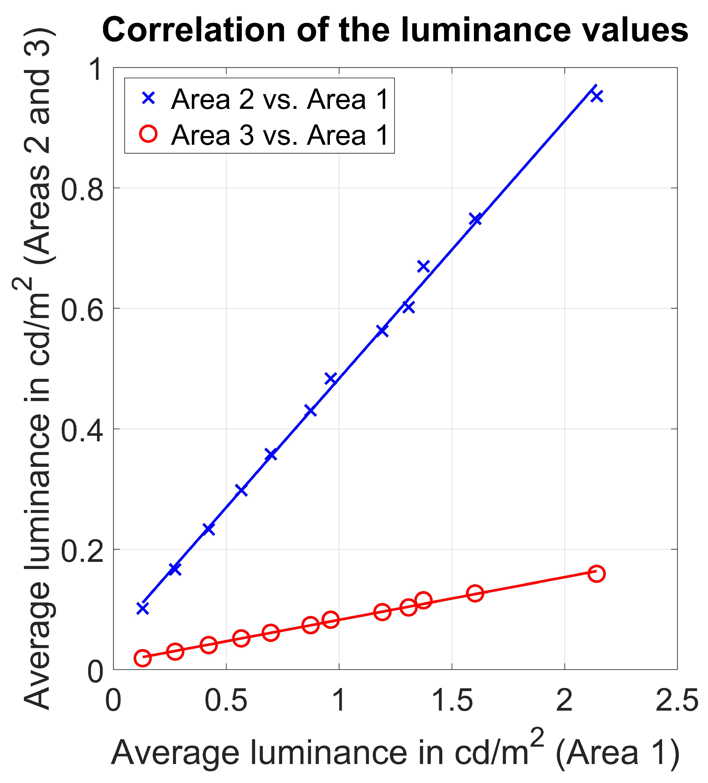
3.1. Forefield Luminance and Its Correlation between Different Evaluation Areas

Figure 4 shows the mean roadway luminance ± standard deviation (Std) of the three different forefield areas (cf. Figure 2 and Figure 3) averaged over the five consecutive test nights as a function of the PWM code values used for driving the LED headlights. Thus, for each combination of evaluation area and PWM code value, the corresponding mean roadway luminance can be extracted and used for further analysis.

Simple linear regression is applied to determine the correlation of the average luminance between the different evaluation areas. As can be seen from Figure 5, there is a significant linear relationship between the average luminance of the near-field and the average luminance of both the mid-field, $r=0.999$, $p<0.001$, $R^2=0.998$, and the far-field, $r=0.998$, $p<0.001$, $R^2=0.996$, where r is the Pearson’s correlation coefficient and $R^2$ denotes the coefficient of determination.

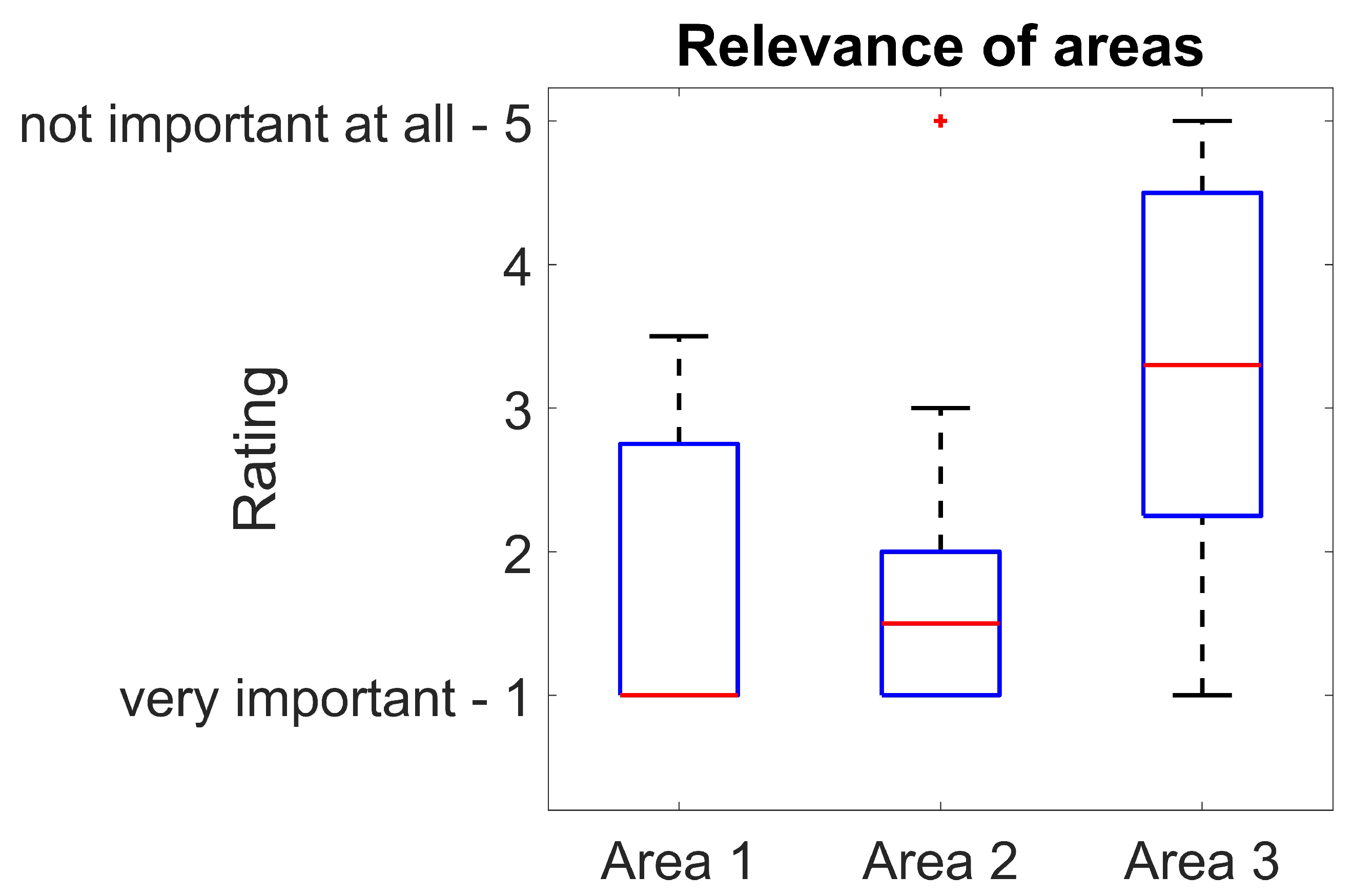
3.2. Relevance of the Different Forefield Areas for Brightness Evaluation

The assessment of the relevance of the different vehicle forefield areas (see Figure 2 and Figure 3) for the evaluation of the subjects’ brightness perception was conducted under static conditions (0 km h⁻¹). The results are summarized in Figure 6. Corresponding box plots illustrate the subjects’ median ratings and quantiles for each of the three different evaluation areas.

Indication is given that the far-field is not as important as the other two evaluation areas. Friedman’s test revealed that the subjects’ relevance ratings significantly differ across evaluation areas, ${\chi }^2\left(2\right)=17.45$, $p<0.001$. Post hoc Wilcoxon signed-rank tests used with Bonferroni correction (adjusted significance level ${\alpha }_{\mathrm{Bonferroni}}=0.0167$) confirmed a statistically significant effect between the far-field area ratings and the ratings obtained for both the near-field, $p<0.001$, $z=-3.34$, and the mid-field area, $p<0.001$, $z=-3.86$. However, there was no significant difference between the near- and the mid-field ratings. Hence, it can be concluded that these two areas of the vehicle’s forefield are equally important with respect to the subjects’ brightness perception, whereas the far-field seems to be less relevant for their evaluation. Both near- and mid-field should therefore be combined in the following to be considered as a single evaluation area that is most crucial for brightness perception while nighttime driving. Again, the average roadway luminace of the combined evaluation area as a function of PWM is determined from the corresponding HDR images as described in Section 2.2.1 and Section 3.1, respectively.

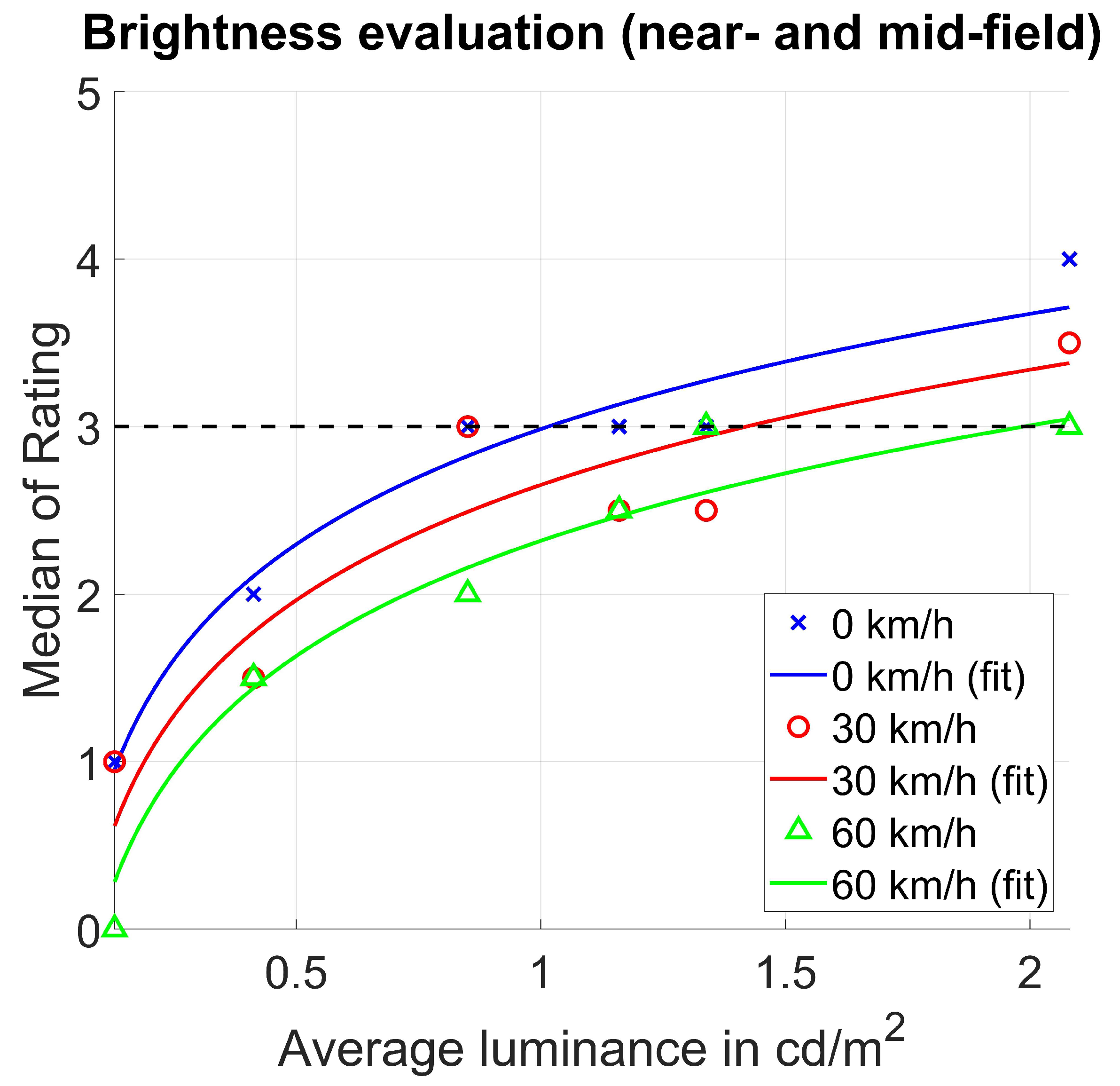
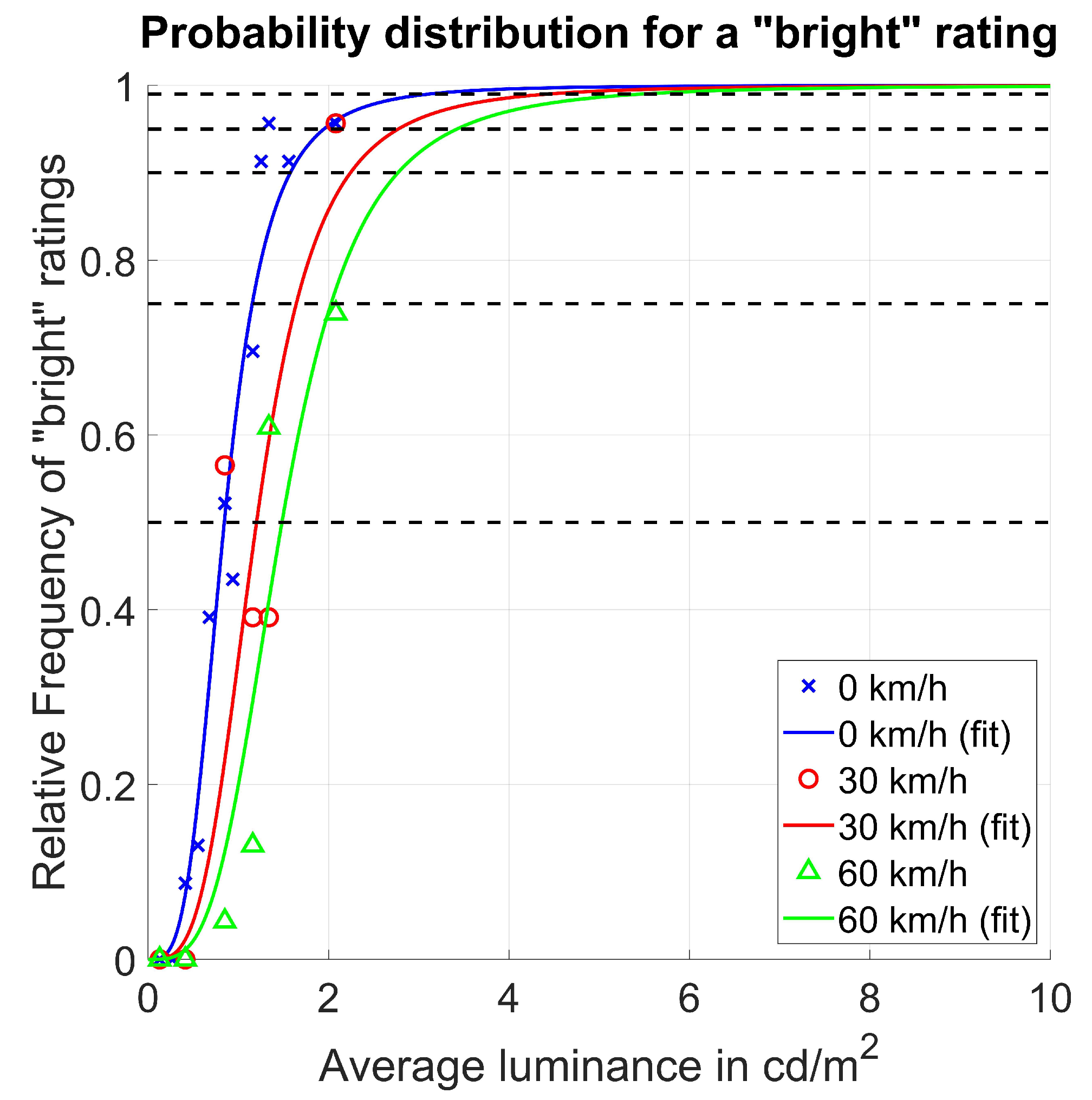
3.3. Speed-Dependent Brightness Evaluation of the Vehicle Forefield

As discussed in the previous section, the luminance data of the combined near- and mid-field evaluation area will be considered for the subsequent analysis since it was identified as most relevant for the assessment of brightness in the vehicle’s forefield, in particular determined by the subjects’ corresponding median relevance ratings depicted in Figure 6. However, it should be emphasized that, due to the linear correlation of the average roadway luminance between the different forefield areas confirmed in Section 3.1, all reported general conclusions and inferences presented here likewise hold for each of the individual evaluation areas without restrictions.

To determine whether a significant correlation between the subjects’ perceived brightness and the average roadway luminance of the combined near- and mid-field evaluation area can be concluded, corresponding Spearman’s correlation coefficients $\rho$ were calculated on their respective median ratings. The results show that there are significantly positive correlations for all three speed levels (static, i.e., 0 km h⁻¹: $\rho =0.94$, $p=0.0167$; 30 km h⁻¹: $\rho =0.85$, $p=0.0491$; 60 km h⁻¹: $\rho =0.99$, $p=0.0056$). For a more detailed examination of these rank correlations, a model function of the form

$$f\left(x\right)=a·log\left(x\right)+b$$

(2)

is used to fit the data. Following the Weber-Fechner law [22], this function approximates human sensory perception and, as such, is hypothesized to be suitable for modeling the present data.

The corresponding results of this model fit applied to the different test conditions are shown in Figure 7. Goodness-of-fit measures are summarized in

Table 1. Goodness-of-fit parameters for the logarithmic fit function at the three velocities ($R^2$: Coefficient of determination, $RMSE$: Root mean squared error). The determined parameters confirm the logarithmic relationship between the roadway luminance and the medians of the brightness rating.

v in km h${}^{-1}$	${\mathit{R}}^2$	$\mathit{RMSE}$
0	0.96	0.21
30	0.82	0.40
60	0.96	0.23

. As expected, the logarithmic relationship between the medians of the subjects’ brightness ratings and the average roadway luminance can clearly be confirmed. Looking at the respective coefficients of determination $R^2$, more than 80% of the variance in the medians of the ratings obtained for different roadway luminances can be explained by the model of Equation (2) at all driving speeds. However, the model predictions appear to be less accurate for the 30 km h⁻¹ condition than for the other two driving conditions. A possible explanation for this finding could be that the subjects experienced more difficulties in judging the degree of appropriateness of the provided forefield brightness at this specific driving speed. While a good consistency was observed in their ratings for both the static and the 60 km h⁻¹ test condition, considerably larger inter-personal deviations were observed for the 30 km h⁻¹ case. Moreover, a conspicuous number of participants occasionally rated a higher forefield luminance to be perceived as darker and, thus, less appropriate to perform the driving task than a lower forfield luminance when driving at 30 km h⁻¹, which again points towards the possible difficulties some of the participants might have in properly judging the lighting conditions at this driving speed. Nevertheless, it should again be emphasized that despite the slightly reduced accuracy observed for the 30 km h⁻¹ test condition, the overall model performance indicated by the Goodness-of-fit measures of Table 1 is still in an acceptable range for all driving speeds considered in this work.

In addition, it should be noted that by applying the proposed model equation the lower feeling of safety threshold luminance of about 1 cd m⁻², which was identified by Kleinkes [36] for his static test conditions as the transition point between “dark” and “bright” ratings, can also be confirmed here. With increasing driving speed, this threshold luminance shifts towards higher values. From Figure 7, it can further be seen that, with increasing driving speed, the median of the brightness evaluation follows a decreasing trend.

Friedman’s test applied to the subjects’ brightness ratings obtained for the different test conditions revealed a significant main effect of driving speed for each of the six different roadway luminance levels. The corresponding p-values and ${\chi }^2$ statistics are tabulated in

Table 2. Results of Friedman’s test for each of the six different average luminance levels of the combined near- and mid-field evaluation area. The results reveal a significant effect of driving speed for all luminance levels.

${\mathit{L}}_{\mathbf{Avg}}$ in cd m${}^{-2}$	${\mathit{\chi }}^2\left(2\right)$	p-Value
0.13	21.59	$2.05 \times {10}^{-5}$
0.41	11.77	$2.80 \times {10}^{-3}$
0.85	24.96	$3.80 \times {10}^{-6}$
1.16	7.89	$1.93 \times {10}^{-2}$
1.34	18.35	$1.04 \times {10}^{-4}$
2.08	15.92	$3.49 \times {10}^{-4}$

. This analysis is limited to those luminance levels used for both static and dynamic testing. Post hoc Wilcoxon signed-rank tests with Bonferroni correction (results are summarized in

Table 3. Test statistics for pairwise comparison of the three velocities at the investigated luminance levels. p-values smaller than the significance level (${\alpha }_{\mathrm{Bonferroni}}$ = 0.0167) indicate luminance levels at which a significant difference between the two compared velocities exists (marked with *).

${\mathit{L}}_{\mathbf{Avg}}$ in in cd m${}^{-2}$	Compared Velocities
	0 km h${}^{-1}$ ↔ 30 km h${}^{-1}$		30 km h${}^{-1}$ ↔ 60 km h${}^{-1}$		0 km h${}^{-1}$ ↔ 60 km h${}^{-1}$
	p	z	p	z	p	z
0.13	$2.54 \times {10}^{-2}$	−2.22	$9.77 \times {10}^{-4}$ *	−3.07	$5.84 \times {10}^{-5}$ *	−4.02
0.41	$2.08 \times {10}^{-2}$	−2.31	$4.30 \times {10}^{-1}$	−0.79	$1.20 \times {10}^{-3}$ *	−3.25
0.85	$1.89 \times {10}^{-1}$	−1.31	$7.33 \times {10}^{-5}$ *	−3.97	$1.80 \times {10}^{-3}$ *	−3.12
1.16	$1.29 \times {10}^{-2}$ *	−2.49	$1.31 \times {10}^{-1}$	−1.51	$4.60 \times {10}^{-3}$ *	−2.83
1.34	$1.89 \times {10}^{-4}$ *	−3.73	$9.67 \times {10}^{-2}$	−1.66	$1.40 \times {10}^{-3}$ *	−3.19
2.08	$2.04 \times {10}^{-1}$	−1.27	$5.21 \times {10}^{-4}$ *	−3.47	$4.63 \times {10}^{-4}$ *	−3.50

) confirmed a statistically significant difference between the two driving speeds at 0 km h⁻¹ and 60 km h⁻¹ for all roadway luminance values. For 0 km h⁻¹ and 30 km h⁻¹ the observed differences are less pronounced. Here, statistically significant deviations can only be concluded for two out of the six different roadway luminance levels used for evaluation. However, with the respective p-values at $0.13$ cd m⁻² and $0.41$ cd m⁻² being close to the Bonferroni-corrected significance level, the potential existence of a true difference in the subjects’ brightness ratings between 0 km h⁻¹ and 30 km h⁻¹ cannot be rejected with sufficient confidence.

A similar conclusion holds when comparing the subjects’ brightness ratings at 30 km h⁻¹ and 60 km h⁻¹, respectively, where differences were significant for three out of the six different roadway luminance settings. Particularly of interest is the noticeable increase of the p-value at an average roadway luminance of $0.41$ cd m⁻². This marks the empirically determined threshold at which more than 91% of the subjects declared to be willing to drive along the test track at both speeds. At lower luminance values, anxiety due to poor light conditions predominated, which resulted in a larger number of subjects refusing to drive, especially for the 60 km h⁻¹ test scenario. Thus, it can be presumed that for most subjects, this absolute minimal safety requirement threshold at $0.41$ cd m⁻² (not to confuse with the lower feeling of safety threshold of Figure 7 or the adequate feeling of safety threshold determined later in this work) defines their personal lower anchor on the respective evaluation scale. Even though they would be willing to drive, they still feel uncomfortable and, in general, demand for higher brightness levels. As a consequence, the subjects’ brightness ratings at this threshold are more or less the same for both velocities showing low variances and equal median values, which leads to the observed highly non-significant post hoc result when testing for differences in brightness perception between 30 km h⁻¹ and 60 km h⁻¹ at a roadway luminance of $0.41$ cd m⁻² as shown in Table 3.

In summary, a significant effect of driving speed on the subjects’ brightness ratings and, thus, on their perception of brightness while driving must be stated. Furthermore, it can be concluded that an average roadway luminance of at least $0.41$ cd m⁻² is required in the vehicle’s combined near- and mid-field area for the subjects to be willing to drive in a country road situation without additional stationary road lighting.

In addition to the provided analysis of medians to explore general trends, it is also of interest to determine, as a function of velocity, the adequate feeling of safety luminance threshold for different speed levels. For this purpose, the relative frequency of “bright” or better ratings (cf. Wagner and Khanh [15]) is determined for each examined roadway luminance as obtained for the three different test conditions at 0 km h⁻¹, 30 km h⁻¹, and 60 km h⁻¹, respectively. The analysis is performed by employing logistic regression, using the psychometric function defined by Linschoten et al. [44]:

$$P\left(x\right)=\gamma +(1-\gamma )·{\displaystyle \frac{1}{1+{{\displaystyle \left(\frac{x}{\alpha }\right)}}^{-\beta }}}$$

(3)

This function is determined by three different parameters, where $\alpha$ represents the stimulus (i.e., the average roadway luminance) with a 50% probability of a positive response (i.e., a “bright” or better rating), $\beta$ defines the steepness of the curve, and $\gamma$ denotes the probability of a positive response occurring simply by chance. In the context of the present study and due to the nature of the stimuli, it is likely that such a random assignment of a “bright” or better rating can be precluded so that $\gamma$ can be set to zero. Hence, the psychometric function of Equation (3) reduces to

$$P_{\gamma =0}\left(x\right)={\displaystyle \frac{1}{1+{{\displaystyle \left(\frac{x}{\alpha }\right)}}^{-\beta }}}$$

(4)

The results of this logistic regression model applied to the different test conditions are shown in Figure 8. The corresponding Goodness-of-fit measures can be obtained from

Table 4. Goodness-of-fit parameters for the logistic regression at the three different driving speed levels ($R^2$: Coefficient of determination, $RMSE$: Root mean squared error). The determined parameters confirm the psychometric relationship between the roadway luminance and the relative frequency of “bright” or better ratings as a function of driving speed.

v in km h${}^{-1}$	${\mathit{R}}^2$	$\mathit{RMSE}$
0	0.96	0.08
30	0.74	0.18
60	0.87	0.12

.

As can be seen, the psychometric model of Equation (4) approximates the data with sufficient accuracy, in particular for the driving speeds of 0 km h⁻¹ and 60 km h⁻¹. At 30 km h⁻¹, the proportion of variance explained by the model is slightly reduced, but with an $R^2$ of 0.74 still in an acceptable range.

Compared to the analysis of the subjects’ median ratings, similar tendencies can be observed here. First, as the average roadway luminance increases, the probability of a “bright” or better rating is also raised for each test condition. Second, with increasing driving speed, the probability of a “bright” or better rating at a given roadway luminance decreases accordingly. From the inverse of the psychometric functions shown in Figure 9, it is further possible to determine the average roadway luminance needed to achieve a certain probability level beyond the standard 50% threshold. To maximize the driver’s general feeling of safety, considerably larger probability thresholds, such as 75%, 90%, or 99%, might be useful in practice.

As shown in Figure 9, for higher probability thresholds beyond 80%, the required roadway luminance increases quite strongly. Again, it can be confirmed that with increasing driving speed, the required roadway luminance for achieving a certain threshold related to “bright” or better ratings also increases. To investigate this effect in more detail and with the goal of extrapolation to higher velocities, a simple linear regression should be performed, including four common probability thresholds, i.e., 50%, 75%, 90%, and 99%. The individual regression curves are shown in Figure 10. The corresponding coefficient of determination is always greater than 0.99, confirming the linear relationship between driving speed and the required roadway luminance to achieve a certain evaluation threshold for “bright” or better ratings to promote an adequate feeling of safety (cf. Wagner and Khanh [15]).

Furthermore, looking at the regression slopes obtained for the different probability thresholds, a steeper increase in the required roadway luminance can be observed at higher thresholds, making them more demanding with regard to proper headlamp design. From the model fits of Figure 10, inter- and extrapolation become possible.

Table 5. Required average roadway luminance values for different probability thresholds at different speed levels. The bold numbers indicate the cases where the used standard LED headlights cannot provide the necessary roadway luminance.

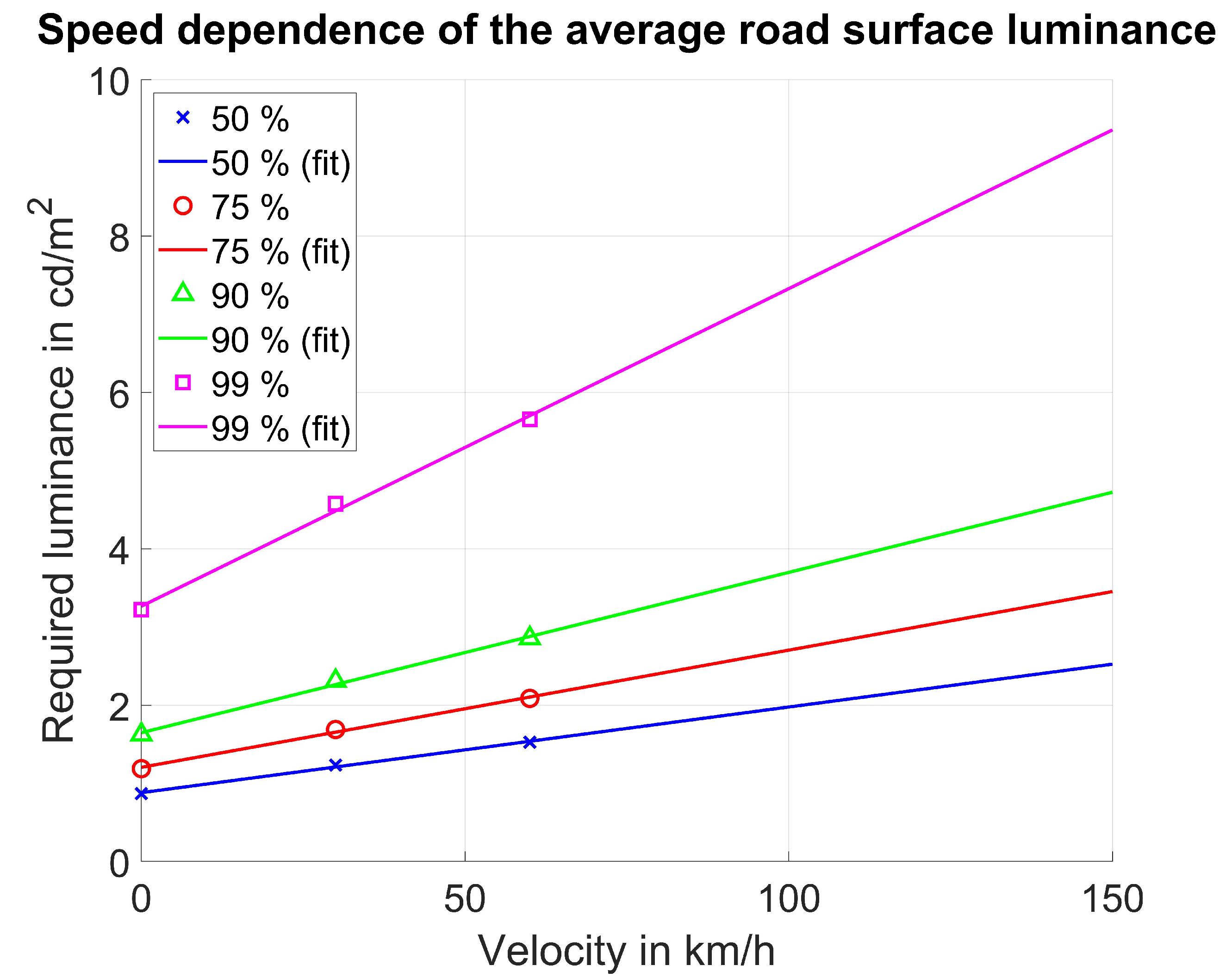
v in km h${}^{-1}$	Required Luminance in cd m${}^{-2}$
	50%	75%	90%	99%
0	0.88	1.21	1.65	3.27
30	1.21	1.65	2.26	4.48
50	1.43	1.95	2.67	5.30
60	1.54	2.10	2.88	5.70
100	1.98	2.70	3.70	7.33
130	2.31	3.15	4.31	8.55

indicates required luminance values for different probability thresholds at some intermediate and higher speed levels as determined from the corresponding regression equations.

As can be seen, for a given probability threshold, an increase in driving speed entails considerably higher roadway luminance values to be required. Note that the maximal average roadway luminance that is feasible in the present study is about $2.08$ cd m⁻². In comparison to Table 5, where bold numbers indicate required roadway luminance values that therefore cannot be achieved with the used headlight system, this means that for example, at a driving speed of 130 km h⁻¹ more than 50% of the subjects would rate the illuminated roadway as “dark” or worse. This results in a significantly diminished feeling of safety and, most likely, reduced object detection performance when driving at such high velocities.

What makes it even more severe is that, except for the static case, at no other speed condition, the roadway would be evaluated as “bright” or better by at least 90% of the subjects. This indicates that standard LED low-beam systems are usually not suited for driving at high velocities that are common on highways and country roads. Even at moderate velocities, the current generation of headlamp systems are anything but optimal so that there is great need for further optimization with respect to subjective safety requirements and objective nighttime driving performance.

3.4. Implications for Urban Areas

Since, in contrast to country roads and highways, stationary road lighting is usually provided in urban areas as an additional source of illumination, the preconditions for headlight systems are somewhat different for these driving situations. According to the European Standard DIN EN 13201-2:2016-06 [45] for urban street lighting, minimum values for the average roadway luminance are defined for several different urban road classes. With a minimum roadway luminance being guaranteed by these regulations, the headlights, in urban-driving situations, are intended to compensate for the differences between the preferred roadway luminance (rated as “bright” or better) to promote an adequate feeling of safety and the roadway luminance provided by the stationary road lighting intended to fulfill legal requirements. As an example, theoretical differences are calculated for a velocity of 50 km h⁻¹, which is the typical speed limit in European urban areas. Results are summarized in

Table 6. Differences determined for achieving the minimum required and preferred roadway luminance values at a velocity of 50 km h⁻¹. The determined differences (columns 6–8) show that for the majority of lighting classes (column 1), a combination of street lighting and dimmed headlights is sufficient to provide the preferred roadway luminance (columns 3–5).

Class	Minimum Average Roadway Luminance ${\mathit{L}}_{\mathbf{m}}$ in cd m${}^{-2}$				Difference to DIN EN 13201 in cd m${}^{-2}$
	DIN EN 13201	Dare to Drive	50%	90%	Dare to Drive	50%	90%
			“Bright”	“Bright”		“Bright”	“Bright”
M1	2.00	0.41	1.43	2.67	−1.59	−0.57	0.67
M2	1.50				−1.09	−0.07	1.17
M3	1.00				−0.59	0.43	1.67
M4	0.75				−0.34	0.68	1.92
M5	0.50				−0.09	0.93	2.17
M6	0.30				0.11	1.13	2.37

.

The second column of Table 6 shows the minimum legal requirements for the roadway luminance provided by stationary road lighting according to the urban road classification system (M-classes; first column) of DIN EN 13201-2:2016-06. The third, fourth, and fifth column tabulate as a reminder the absolute minimum required roadway luminance for a test person to be willing to drive a vehicle as well as the approximated luminance values of the probability thresholds in brightness perception for 50% and 90% “bright” or better ratings, as derived from the present study for a velocity of 50 km h⁻¹. Finally, for each road class, the differences between these three luminance threshold values and the DIN EN 13201-2:2016-06 requirements for stationary road lighting are summarized in the three last columns of Table 6.

Negative differences indicate that the threshold luminance values are already exceeded by the legally required minimal roadway luminance that must be guaranteed by the stationary road lighting installation for a specific urban road class. In these cases, the headlamps’ low-beam function contributes to an increased driving comfort and feeling of safety by providing an additional illumination of the roadway. This is particularly important in cases where the DIN EN 13201-2:2016-06 requirements are just bright enough for a motorist to be willing to drive a vehicle but do not really contribute to an adequate safety perception (e.g., in case of M4 and M5). The positive differences shown in italic further indicate those roadway classes for which the low-beam function of the headlight system used in the present study can be dimmed in such a way that the perceptual threshold requirements can be achieved by combining the individual contributions of the stationary road lighting and the vehicle’s headlamps. The bold numbers, on the other hand, highlight those roadway classes for which even the full low beam output (i.e., $L_{\mathrm{Avg,max}}$ = $2.08$ cd m⁻²) of the headlight system used in the present study is not sufficient to achieve the respective threshold luminance on the roadway even though stationary road lighting is provided. In those cases, further optimization of the low-beam function seems to be also indicated for urban areas.

Note that for this theoretical consideration, an utterly homogeneous illumination of the roadway provided by the stationary road lighting is assumed, which, of course, rarely occurs in real-world situations. Furthermore, the theoretical consideration is carried out under the assumption of a completely dark surrounding with no other light sources being present, which of course is also not the case in the real world. Thus, further investigations in urbanized areas are required to validate these results and to transfer them into practice.

4. Conclusions and Outlook

This work was intended to quantitatively assess the driver’s brightness perception of the vehicle forefield with regard to an adequate feeling of safety as a function of roadway luminance provided by the vehicle’s headlight system and driving speed. In particular, the explicit inclusion of dynamic driving situations extends the current knowledge in this field of research, which, so far, was derived from laboratory studies and static experiments only. Based on the collected rating data, it was found that a range of up to 32 $\mathrm{m}$ in front of the vehicle is relevant for the general perception of brightness. In addition, it could be shown that an absolute minimal average roadway luminance of $0.41$ cd m⁻² is required in this forefield area for a driver to be willing to perform a driving task.

In the static case, the average roadway luminance should be at least $0.88$ cd m⁻² so that every second driver evaluates the roadway as “bright” or better, a rating that based on the literature is associated with an adequate feeling of safety regarding nighttime driving. At higher velocities, this roadway luminance must be increased accordingly (i.e., for 30 km h⁻¹ to $1.21$ cd m⁻² and 60 km h⁻¹ to $1.54$ cd m⁻²) to still ensure the 50% probability threshold. If, on the other hand, the probability of a “bright” or better rating should be increased to a considerably higher value, for example, to 99%, the corresponding roadway luminance must be strongly enhanced. Compared to the 50% probability threshold, a factor of approximately 3.7 is required independent of the driving speed, which usually cannot be achieved with the low-beam function of standard LED headlamps. As the experimental setting of the present work represents a single driving scenario of a countryside roadway (i.e., no stationary lighting) with two lanes of constant width, the question arises whether different environmental test conditions may affect the subjects’ rating results. Potential impact factors that need to be considered for a comprehensive evaluation are for example the width of the lanes, the road and lane markings, as well as the roadway surroundings including reflector posts and street signs. Another factor that may have a direct impact on the subjects’ feeling of safety while nighttime driving and, thus, affect their corresponding ratings is the topological nature of the course of the road. It is for example likely that it makes a difference whether the driving task is performed in a flat or in a rather hilly environment. Hence, further experiments will be required—preferably to be conducted in real-world traffic situations—in order to be able to draw corresponding conclusions.

Based on theoretical considerations for urban areas, it could at least be shown that in German and European cities, where the typical driving speed is limited to 50 km h⁻¹, a combination of stationary road lighting and dimmed low-beam distribution is sufficient to meet the considered threshold requirements in preferred roadway luminance for the majority of road classes defined by DIN EN 13201-2:2016-06. However, in some of these cases, particularly regarding the 90% probability threshold, even the combination of stationary road lighting and the vehicle’s low-beam distribution driven at maximal intensity was insufficient to meet the corresponding minimum requirements for an adequate brightness perception, which is expected to considerably diminish the drivers’ feeling of safety in these situations.

Thus, concerning future research and practice, it is crucial to develop and optimize new low-beam systems that are capable of providing higher roadway luminance values than the standard LED headlamps that are used today, of course, without introducing additional sources of glare. Furthermore, the experiments should be repeated for urban areas, including stationary road lighting, to validate the theoretical considerations of Section 3.4. The present study was conducted with a group of younger drivers recruited from university, which introduces a certain bias in the reported results in case one attempts to generalize them to a more global population. Thus, future studies should likewise include older drivers to explicitly consider the age dependency of brightness perception as a probably important impact factor. In addition, larger sample sizes may also increase statistical power, which is especially important for the exploration of higher-order interaction effects such as between gender or driving speed and age.

Finally, this work also creates the basis for subsequent considerations on potential energy savings and the adaptation of regulations for current and future adaptive headlight systems. With such future systems being capable of automatically adapting to the environmental conditions, an energy-efficient lighting concept could be developed that is suitable for satisfactory forefield lighting on both illuminated and unilluminated roads while still promoting an adequate feeling of safety. To define system requirements for a reliable detection of objects, corresponding contrast thresholds must be investigated and defined accordingly.

References

- Sivak, M. The information that drivers use: Is it Indeed 90 % visual? Perception 1996, 25, 1081–1089. [Google Scholar] [CrossRef]
- Charman, W.N. Vision and driving—A literature review and commentary. Ophthalmic Physiol. Opt. 1997, 17, 371–391. [Google Scholar] [CrossRef]
- Diem, C. Blickverhalten von Kraftfahrern im Dynamischen Straßenverkehr; Darmstädter Lichttechnik, Utz: München, Germany, 2005. [Google Scholar]
- Underwood, G. Visual attention and the transition from novice to advanced driver. Ergonomics 2007, 50, 1235–1249. [Google Scholar] [CrossRef]
- Statistisches Bundesamt. Verkehrsunfälle-Zeitreihen—2019. 2020. Available online: https://www.destatis.de/DE/Themen/Gesellschaft-Umwelt/Verkehrsunfaelle/Publikationen/Downloads-Verkehrsunfaelle/verkehrsunfaelle-zeitreihen-pdf-5462403.html (accessed on 20 May 2021).
- Scott, P.P. The Relationship Between Road Lighting Quality and Accident Frequency; TRRL Laboratory Report; Transport and Road Research Laboratory: Crowthorne, UK, 1980. [Google Scholar]
- Sullivan, J.M.; Flannagan, M.J. The role of ambient light level in fatal crashes: Inferences from daylight saving time transitions. Accid. Anal. Prev. 2002, 34, 487–498. [Google Scholar] [CrossRef]
- Oya, H.; Ando, K.; Kanoshima, H. A research on interrelation between illuminance at intersections and reduction in traffic accidents. J. Light Vis. Environ. 2002, 26, 29–34. [Google Scholar] [CrossRef] [Green Version]
- Bullough, J.D.; Donnell, E.T.; Rea, M.S. To illuminate or not to illuminate: Roadway lighting as it affects traffic safety at intersections. Accid. Anal. Prev. 2013, 53, 65–77. [Google Scholar] [CrossRef]
- Jackett, M.; Frith, W. Quantifying the impact of road lighting on road safety—A New Zealand study. IATSS Res. 2013, 36, 139–145. [Google Scholar] [CrossRef] [Green Version]
- Fotios, S.; Gibbons, R. Road lighting research for drivers and pedestrians: The basis of luminance and illuminance recommendations. Light. Res. Technol. 2018, 50, 154–186. [Google Scholar] [CrossRef]
- Schlag, B.; Petermann, I.; Weller, G.; Schulze, C. Mehr Licht–mehr Sicht–mehr Sicherheit? Zur Wirkung verbesserter Licht- und Sichtbedingungen auf das Fahrerverhalten; VS Verlag für Sozialwissenschaften: Wiesbaden, Germany, 2009. [Google Scholar] [CrossRef]
- Eby, D.W.; Molnar, L.J.; Zhang, L.; St. Louis, R.M.; Zanier, N.; Kostyniuk, L.P.; Stanciu, S. Use, perceptions, and benefits of automotive technologies among aging drivers. Inj. Epidemiol. 2016, 3, 28. [Google Scholar] [CrossRef] [Green Version]
- Setyaningsih, E.; Suryo Putranto, L.; Soegijanto, R.; Soelami, F.X.N. Analysis of the visual safety perception and the clarity of traffic signs and road markings in the presence of road lighting in straight and curved road. MATEC Web Conf. 2018, 181, 04001. [Google Scholar] [CrossRef] [Green Version]
- Wagner, M.; Khanh, T.Q. Sicher durch die nächtliche Stadt–Helligkeits- und Kontrastwahrnehmung in der städtischen Straßenbeleuchtung aus Fahrersicht. Licht 2020, 72, 108–113. [Google Scholar]
- Wördenweber, B.; Lachmayer, R.; Witt, U. Intelligente Frontbeleuchtung. ATZ Automob. Z. 1996, 98, 546–551. [Google Scholar]
- Kosmas, K. Optimierung von adaptiven Kfz-Scheinwerfertechnologien zur Blendungsbegrenzung unter dynamischen Bedingungen. Ph.D. Thesis, Technical University of Darmstadt, Darmstadt, Germany, 2019. Available online: https://tuprints.ulb.tu-darmstadt.de/8747/ (accessed on 25 October 2021).
- Stamatiadis, N.; Psarianos, B.; Apostoleris, K.; Taliouras, P. Nighttime versus daytime horizontal curve design consistency: Issues and concerns. J. Transp. Eng. Part A Syst. 2020, 146, 04019080. [Google Scholar] [CrossRef]
- Plainis, S.; Murray, I.J.; Pallikaris, I.G. Road traffic casualties: Understanding the night-time death toll. Inj. Prev. 2006, 12, 125–128. [Google Scholar] [CrossRef] [Green Version]
- Wanvik, P.O. Effects of road lighting: An analysis based on Dutch accident statistics 1987–2006. Accid. Anal. Prev. 2009, 41, 123–128. [Google Scholar] [CrossRef]
- Damasky, J. Lichttechnische Entwicklung von Anforderungen an Kraftfahrzeugscheinwerfer. Ph.D. Thesis, Technische Hochschule Darmstadt, Darmstadt, Germany, 1995. [Google Scholar]
- Fechner, G.T. Elemente der Psychophysik: Erster Theil; Breitkopf und Härtel: Leipzig, Germany, 1860. [Google Scholar]
- Schmidt-Clausen, H.J.; Freiding, A. Sehvermögen von Kraftfahrern und Lichtbedingungen im nächtlichen Straßenverkehr. In Berichte der Bundesanstalt für Straßenwesen M, Mensch und Sicherheit; Wirtschaftsverl. NW Verl. für neue Wiss: Bremerhaven, Germany, 2004; Volume 158. [Google Scholar]
- Plainis, S.; Murray, I.J. Reaction times as an index of visual conspicuity when driving at night. Ophthalmic Physiol. Opt. 2002, 22, 409–415. [Google Scholar] [CrossRef]
- Graf, C.P.; Krebs, M.J. Headlight Factors and Nighttime Vision: Final Report; DOT HS-802 102; U.S. Department of Transportation, National Highway Traffic Safety Administration: Washington, DC, USA, 1976.
- Chmielarz, M.; Schneider, W.; Sprenger, A.; Theil, L. Blickverteilung beim Fahren in PKW bei Nacht. In Blickfixationen und Blickbewegungen des Fahrzeugführers sowie Hauptsichtbereiche an der Windschutzscheibe (FAT-Schriftenreihe Nr. 151); Brückmann, R., Ed.; Verband der Automobilindustrie e. V. (VDA): Berlin, Germany, 2000; pp. 43–59. [Google Scholar]
- Garay-Vega, L.; Fisher, D.L.; Pollatsek, A. Hazard anticipation of novice and experienced drivers: Empirical evaluation on a driving simulator in daytime and nighttime conditions. Transp. Res. Rec. 2007, 2009, 1–7. [Google Scholar] [CrossRef]
- Cengiz, C.; Kotkanen, H.; Puolakka, M.; Lappi, O.; Lehtonen, E.; Halonen, L.; Summala, H. Combined eye-tracking and luminance measurements while driving on a rural road: Towards determining mesopic adaptation luminance. Light. Res. Technol. 2014, 46, 676–694. [Google Scholar] [CrossRef]
- Grüner, M.; Ansorge, U. Mobile eye tracking during real-world night driving: A selective review of findings and recommendations for future research. J. Eye Mov. Res. 2017, 10, 1–18. [Google Scholar] [CrossRef]
- Kobbert, J. Optimization of Automotive Light Distributions for Different Real Life Traffic Situations. Ph.D. Thesis, Technical University of Darmstadt, Darmstadt, Germany, 2019. Available online: https://tuprints.ulb.tu-darmstadt.de/8382/ (accessed on 25 October 2021).
- Cohen, A.S.; Hirsig, R. Zur Bedeutung des Fovealen Sehens für die Informationsaufnahme bei hoher Beanspruchung. In Sicht und Sicherheit im Straßenverkehr–Beiträge zur interdisziplinären Diskussion; Derkum, H., Ed.; Verlag TÜV Rheinland: Köln, Germany, 1990; pp. 47–58. [Google Scholar]
- Damasky, J.; Hosemann, A. The Influence of the Light Distribution of Headlamps on Drivers Fixation Behaviour at Nighttime; SAE Technical Paper Series; SAE International 400 Commonwealth Drive: Warrendale, PA, USA, 1998. [Google Scholar] [CrossRef]
- Brückmann, R.; Gottlieb, W.; Hatzius, J.; Hosemann, A.; Reitter, C.; Rößger, P. Blickbewegungen des Fahrers bei Nacht bei alternativen Kfz-Scheinwerfern. In Blickfixationen und Blickbewegungen des Fahrzeugführers sowie Hauptsichtbereiche an der Windschutzscheibe (FAT-Schriftenreihe Nr. 151); Brückmann, R., Ed.; Verband der Automobilindustrie e. V. (VDA): Berlin, Germany, 2000; pp. 107–187. [Google Scholar]
- Hamm, M.; Friedrich, A. Intelligente, adaptive Scheinwerfersysteme: Die Fahrzeug-Außenbeleuchtung der Zukunft. ATZ Automob. Z. 2000, 102, 1042–1047. [Google Scholar] [CrossRef]
- Schreuder, D.A. Straßenbeleuchtung für Sicherheit und Verkehr; Shaker: Aachen, Germany, 2001. [Google Scholar]
- Kleinkes, M. Objektivierte Bewertung des Gütemerkmals Homogenität für Scheinwerfer-Lichtverteilungen, 1st ed.; Berichte aus der Physik, Shaker: Aachen, Germany, 2003. [Google Scholar]
- Loewen, L.J.; Steel, G.D.; Suedfeld, P. Perceived safety from crime in the urban environment. J. Environ. Psychol. 1993, 13, 323–331. [Google Scholar] [CrossRef]
- Boyce, P.R.; Eklund, N.H.; Hamilton, B.J.; Bruno, L.D. Perceptions of safety at night in different lighting conditions. Light. Res. Technol. 2000, 32, 79–91. [Google Scholar] [CrossRef]
- Blöbaum, A.; Hunecke, M. Perceived Danger in Urban Public Space. Environ. Behav. 2005, 37, 465–486. [Google Scholar] [CrossRef]
- Haans, A.; de Kort, Y.A. Light distribution in dynamic street lighting: Two experimental studies on its effects on perceived safety, prospect, concealment, and escape. J. Environ. Psychol. 2012, 32, 342–352. [Google Scholar] [CrossRef]
- Boomsma, C.; Steg, L. Feeling Safe in the Dark. Environ. Behav. 2014, 46, 193–212. [Google Scholar] [CrossRef]
- Fotios, S.; Unwin, J.; Farrall, S. Road lighting and pedestrian reassurance after dark: A review. Light. Res. Technol. 2015, 47, 449–469. [Google Scholar] [CrossRef] [Green Version]
- Peña-García, A.; Hurtado, A.; Aguilar-Luzón, M.C. Impact of public lighting on pedestrians’ perception of safety and well-being. Saf. Sci. 2015, 78, 142–148. [Google Scholar] [CrossRef]
- Linschoten, M.R.; Harvey, L.O.; Eller, P.M.; Jafek, B.W. Fast and accurate measurement of taste and smell thresholds using a maximum-likelihood adaptive staircase procedure. Percept. Psychophys. 2001, 63, 1330–1347. [Google Scholar] [CrossRef]
- Deutsches Institut für Normung, e.V. DIN EN 13201-2:2016-06, Straßenbeleuchtung—Teil 2: Gütemerkmale; Deutsche Fassung (EN 13201-2:2015); Deutsches Institut für Normung e.V. (DIN): Berlin, Germany, 2016. [Google Scholar] [CrossRef]