An Approach to the Definition of the Aerodynamic Comfort of Motorcycle Helmets

Abstract

The aim of this work is to obtain a reliable testing methodology for the characterization of the perceived aerodynamic comfort of motorcycle helmets. Attention was paid to the rider’s perception of annoying vibrations induced by wind. In this optic, an experimental comparative campaign was performed in the wind tunnel, testing 16 helmets in two different configurations of neck stiffness. The dataset was collected within a convolutional neural network (CNN or ConvNet) of images, creating a ranking by identifying the best and the worst helmets. The results revealed that each helmet has unique aerodynamic characteristics. Depending on the ranking scale previously created, the aerodynamic comfort of each helmets can be classified within the scale.

1. Introduction

Driving comfort is sensitive to various boundary conditions. Aspects such as perceived noise, annoying vibrations transmitted by the vehicle and the thermal conditions of the driver represent three macro areas on which the automotive industry has focused a lot in recent years. When driving a vehicle, the overall comfort feeling is given by the contributions of noise (structural noise and aeroacoustics noise), induced vibrations and driving thermal conditions. In general, the participation ratio of each of the previous contribution to the global feeling is somewhat related to the speed of the vehicle. Moreover, depending on the type of vehicle, some aspects become predominant over the others. For passenger cars, over 70 km/h [1,2], interior noise is one of the main aspects for defining perceived comfort. If dealing with tracks or operating machines, isolation of the driver from vibrations, due to the huge power units, is of primary necessity. In these cases, thermal comfort is guaranteed by efficient air conditioning systems. In the case of motorcycles, the driver becomes an active part of the aerodynamical system; hence, a large amount of the perceived comfort is related to aerodynamics. If we restrict the field of analysis to the motorcycle helmet case, aerodynamics alone is responsible for noise (aeroacoustics noise), annoying vibrations and thermal comfort. It goes without saying that the design of “a first of all safe and then comfortable helmet” is challenging from different standpoints. Several research campaigns have been carried out on topics concerning the aerodynamics of the “Motorcycle-Rider” system [3] or in order to improve the vehicle’s drag resistance [4]. Although there is a certain correlation between noise and vibration (vortex shedding very often produces noise), from the engineering point of view it is legitimate to separate the effects, optimizing the perceived noise, vibrational and thermal aspects separately.

When dealing with wind load-induced vibrations on the helmet of the rider, reference is made to the biomechanics side [5]. It should be noted that vibrations at low frequencies, in the range between 0.1 and 20 Hz, are annoying for the human body. The damaging potential of a vibrating source, to which the human body responds, is dependent on several factors such as: “The physical characteristics of the vibrating source such as frequency and acceleration; The direction of propagation of vibrations along the biodynamic axes; The duration of exposure to the vibrating source; Characteristic frequency of individual organs; Damping characteristics, impedance and transmissibility of the tissues; Posture of the human body” [6].

Numerous mathematical models have been introduced in order to evaluate the behavior of the human body and the effect of vibrations over it; for example through concentrated parameter models or finite element models [7]. However, the most used model is the Griffin model [8,9].

The perception of vibrations by the human body is purely subjective and influenced by the case studies chosen to perform the examination. Many researchers have tried to evaluate the comfort level on various types of vehicles adopting sinusoidal inputs. The sensations reported by the human samples subject to these vibrations have been labelled with a level of comfort through a numerical judgment [10,11,12,13,14,15].

Low-frequency vibrations interfere with the function of the vestibular apparatus, causing phenomena of motion sickness, dizziness and proprioception disorders of the body. In the transverse direction, the most annoying vibration frequencies for the human body are those of 1–2 Hz; in the vertical one (feet–head) instead the more annoying are those between 4 and 8 Hz [16,17,18,19,20].

It is possible to classify the effects of vibrations on humans according to a progressive scale of danger distributed in the following levels of disturbance: fatigue, interference with efficiency and performance and damage. Three different aspects should be considered: duration, amplitude and frequency of excitement. These three factors contribute to absorption in different ways and in combination with each other. For example, a vibration of low amplitude and prolonged over time can be equivalent in danger to a greater and shorter amplitude [21].

The knowledge of the human body characteristics and its behavior following dynamic stresses is also fundamental to prevent consequences that could undermine its health. In this research area, different categories of models are generally used: volunteers, corpses, animals, mechanical models and mathematical models [22].

Among mathematical models, Dieckmann in 1958 [23] proposed a five-degree linear model of freedom to study the dynamic response of the chest and internal organs. Coermann [24,25] described a simplified seven-mass model to describe the vibrational dynamics of a person standing or sitting. Chaffin in 1969 [26], on the other hand, created a static model with seven segments to estimate the loads deriving from the manipulation of some objects. Ten years later, Gruver [27] proposed a two-dimensional five-segment model. In 1970 Kane and Scher [28] modelled a three-segment system with the aim of studying how to obtain body rotations in space by means of appropriate movements of the limbs. Passerello and Huston [29] developed a 10-segment model to simulate the human body in space.

Regarding the vibrational study, linked to the neck–head system of the individual following the impact with the incident flow during the vehicle motion, reference is made to ISO 2631 [30,31,32]. The use of the following standard is used as an initial starting point of the study. Starting from it, the authors try to characterize the phenomenon of vibrations.

In the aforementioned field of interest, the effects of vibrations are more linked to exposure time than to the amplitude of the vibrations considered. In transport, vibrational stresses never reach harmful levels under ordinary conditions. The purpose of this work is to approach the definition of the comfort for motorcycle helmets to lead the companies in the product design phase. An experimental testing campaign in the wind tunnel was designed, analyzing the vibration time histories of 16 different motorcycle helmets, along three different axes.

Tests were performed with two different neck stiffnesses and acceleration data were processed by a methodology based on neural networks. Finally, a ranking was drawn up relating to the comfort index of each helmet under analysis.

2. Materials and Methods

2.1. The Wind Tunnel Facilities

The experimental activity for the determination of the comfort coefficient, was carried out inside the “R. Balli” wind tunnel of the University of Perugia [4] which presented a closed-circuit configuration with an open test section.

The measurement of aerodynamic loads was given by a scale that uses 6-component load cells which allows for the decomposition of forces and moments in the three main directions of the reference system. The signals produced by the force, pressure and temperature transducers were acquired by a National Instruments BNC-2090 card. The program that managed data acquisition, saved, and provided a user interface was realized with the National Instruments LABVIEW^® software.

The acquisition system consisted of two triaxial accelerometers, PCB 356A15 and LGA-16L, respectively, and a PCB 353B44 monoaxial accelerator from PCB Piezotronics.

In the first analysis, these tools were used to characterize which acceleration component was the greatest in intensity. Finally, the sound level meter was used to find a correlation between acceleration and pressure.

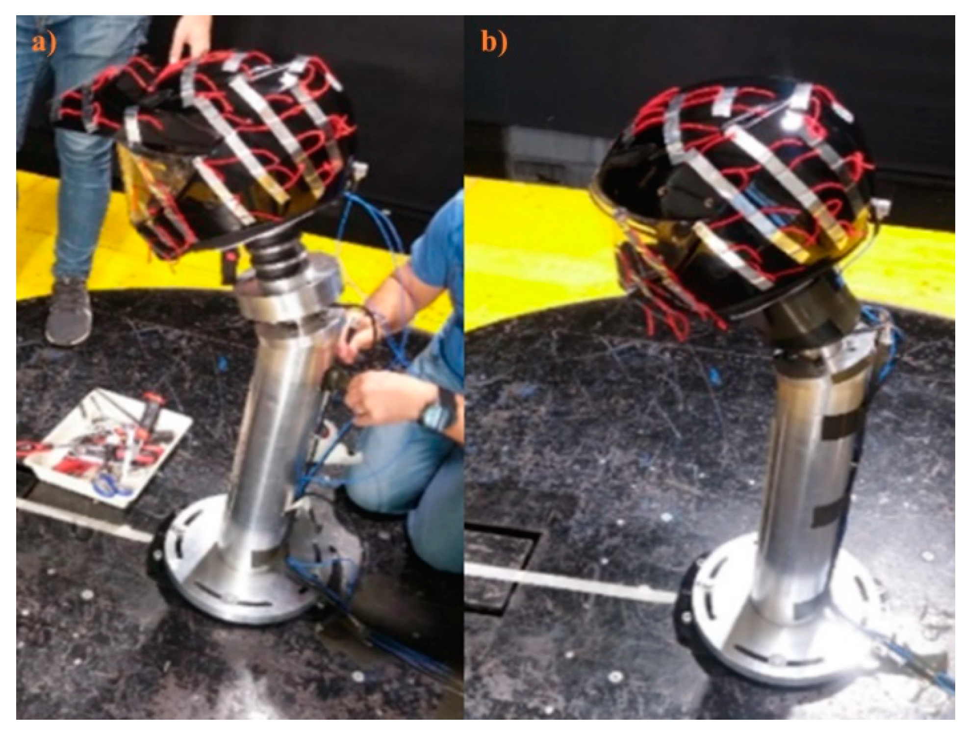
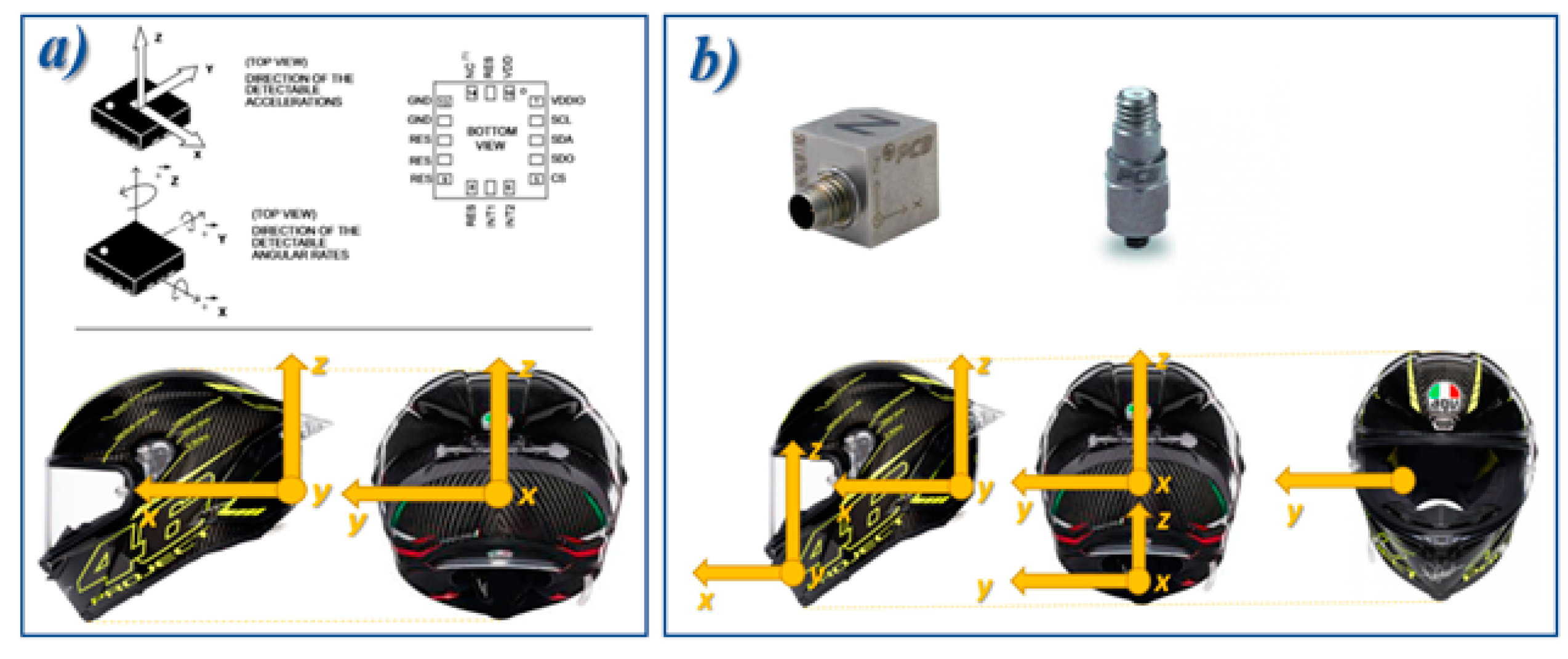
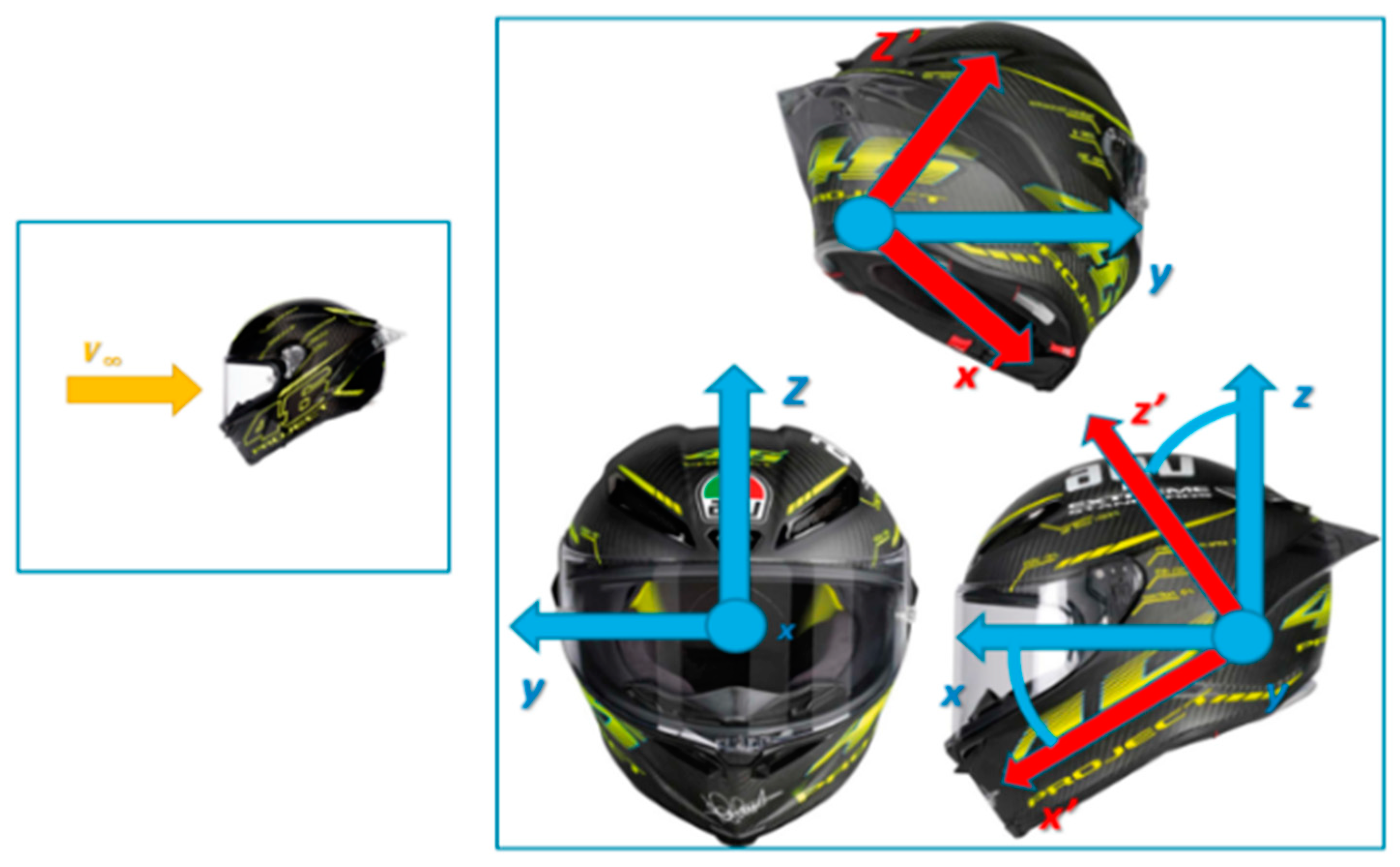
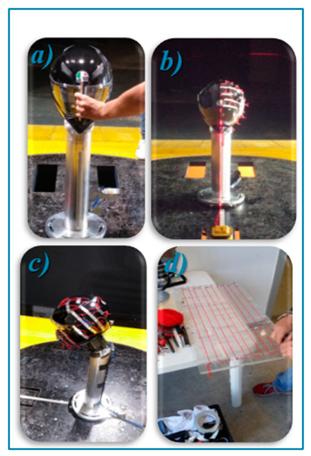
2.2. The Experimental Setup

The wind tunnel tests were divided according to the type of neck support system adopted (Figure 1). The tests were classified into two types:

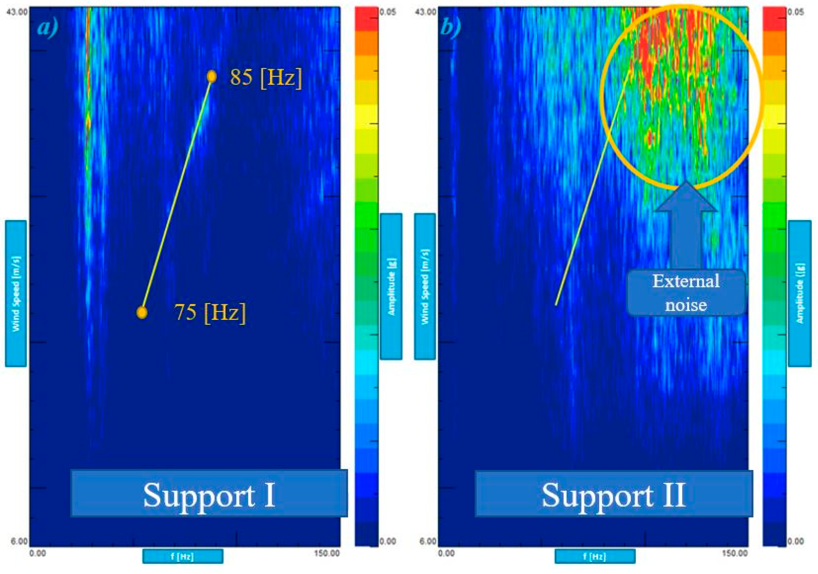
• Support I: Hybrid 3. It was made up of aluminum discs interposed with rubber discs, which represent the vertebrae and that confers to the manikin neck a very similar response to that of the human neck, without the need of having to use a human subject to carry out the tests.
• Support II: Rigid. The effects related to the stiffness of the neck-head system are neglected.

The tests are indicated from A to D. In the first three analysis campaigns (Test A, Test B and Test C), only one triaxial accelerometer “LGA-16L” was used, positioned as shown in Figure 2a. The most affected component by aerodynamic effects was isolated. For this reason, an accelerometer was placed on the front of the helmet and the sound level meter was used to correlate acoustic and aerodynamic effects. On the other hand, for Test D, a triaxial accelerometer (PCB 356°15) mounted on the back of the helmet, a monoaxial accelerometer (PCB 353B44) mounted on the visor and the sound level meters (Gras 40a0) connected inside the shell were used as shown in Figure 2b.

The helmet was aligned to the vertical axis, as shown in Figure 3 and Figure 4a.

The helmet was cantered with the aim of obtaining an angle of 0° compared to the other two axes, in order to simulate a condition in which the wind speed is directed towards the helmet (Figure 4b). In Test D, woolen threads were also used to characterize the wind flow around the helmet (Figure 4c,d).

Table 1. Test’s summary.

	Test A	Test B	Test C
Number of helmets chosen	4	5	5
Used neck	Hybrid 3	Rigid neck	Rigid neck
Time interval duration	30 s	30 s	30 s
Wind speed	160 km/h	160 km/h	Ramped (0–160 km/h)
Monoaxial accelerometer	//	//	PCB 353B44
Triaxial accelerometer	LGA-16L	LGA-16L	PCB 356A15
Sound level meter	//	//	G.r.a.s. 40a0

summarizes the setups relating to the four tests.

3. Theoretical background

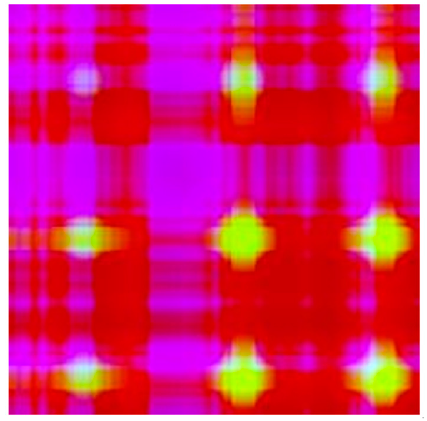
3.1. Gramian Angular Field

The Gramian Angular Summation Field (GASF) and Gramian Angular Difference Field (GADF) are two techniques that encode time series signals into an image. The concept was, therefore, to transfer the time series in a polar coordinate space, rather than in a Cartesian coordinate system. This is mathematically explained as follows. For n observations evaluated as real in a time series.

x = x₁, x₂, ..., x_n

(1)

The latter are first normalized between −1 and 1 as:

$$\overline{\mathrm{x}}=\frac{\left({\mathrm{x}}_{\mathrm{i}}-\max (\mathrm{x})\right)+\left({\mathrm{x}}_{\mathrm{i}}-\min (\mathrm{x})\right)}{\max (\mathrm{x})-\min (\mathrm{x})}$$

(2)

The next step was to obtain the polar coordinates: the angle ϕ of the cosine, with normalized amplitude values; the radius r, obtained from the time history t [33].

$$\{\begin{array}{c}\mathsf{\varphi }=\mathrm{a}\mathrm{r}\mathrm{c}\mathrm{o}\mathrm{s}\left(\overline{{\mathrm{x}}_{\mathrm{i}}}\right),-1\le \overline{{\mathrm{x}}_{\mathrm{i}}}\le 1,\overline{{\mathrm{x}}_{\mathrm{i}}}\in \bar{\mathrm{X}}\\ \mathrm{r}=\frac{{\mathrm{t}}_{\mathrm{i}}}{\mathrm{N}},{\mathrm{t}}_{\mathrm{i}}\in \mathrm{N}\end{array}$$

(3)

$\bar{\mathrm{X}}$ represents the time series, ${\mathrm{t}}_{\mathrm{i}}$ represents the time step and N is a constant factor to regularize the arc of the polar coordinate system. The representation of polar coordinates has two main characteristics:

• One-to-one mapping of the time series to the results of the polar coordinates; therefore, it is bijective.
• The temporal relationships are preserved.

The polar coordinates of the time series normalized in the interval (−1,1) fell within the boundaries between (0,π). This provided different concentrations of information in the GASF, which should aid the fibber filtration process. Finally, once the change of coordinates was obtained, it was proceeded with the composition of the matrices of GASF, GADF.

$$\mathrm{GASF}=\left[\begin{array}{c}\begin{array}{ccc}{\cos (\Phi }_1{+\Phi }_1)& \cdots & {\cos (\Phi }_1{+\Phi }_{\mathrm{n}})\end{array}\\ \begin{array}{ccc}{\cos (\Phi }_2{+\Phi }_1)& \cdots & {\cos (\Phi }_2{+\Phi }_{\mathrm{n}})\\ ⋮& \ddots & ⋮\\ {\cos (\Phi }_{\mathrm{n}}{+\Phi }_1)& \cdots & {\cos (\Phi }_{\mathrm{n}}{+\Phi }_{\mathrm{n}})\end{array}\end{array}\right]$$

(4)

$$\mathrm{GADF}=\left[\begin{array}{c}\begin{array}{ccc}{\sin (\Phi }_1{-\Phi }_1)& \cdots & {\sin (\Phi }_1{-\Phi }_{\mathrm{n}})\end{array}\\ \begin{array}{ccc}{\sin (\Phi }_2{-\Phi }_1)& \cdots & {\sin (\Phi }_2{-\Phi }_{\mathrm{n}})\\ ⋮& \ddots & ⋮\\ {\sin (\Phi }_{\mathrm{n}}{-\Phi }_1)& \cdots & {\sin (\Phi }_{\mathrm{n}}{-\Phi }_{\mathrm{n}})\end{array}\end{array}\right]$$

(5)

There are several advantages related to the use of this method. From the main diagonal, the neural networks manage to reconstruct the main features. The GASF matrix (n × n) is used as an image for the classifier. However, the complexity of calculation can increase due to the large size of the image as it depends on the length of the time series. Therefore, the image was resized and reduced to a comfortable 224 × 224 standard. This was performed by applying a scaling to the original image. Bicubic interpolation is a method of resizing the image, in which the value of the output pixel is a weighted average calculated on a 4 × 4 neighborhood that surrounds the input pixel. This method produces a uniform image compared to other interpolation methods and is popular in many image processing algorithms [34].

3.2. Experimental Computer Analysis

The first step was represented by the creation of an algorithm capable of carrying out a transformation from time to frequency domain for the analyzed signal. To obtain this result, the Fast Fourier Transform (FFT) was used. The algorithm was created using the MathWorks MATLAB^® program. The first cases analyzed were represented by sinusoids of varying frequency in order to test the effectiveness of the algorithm. Once the accuracy was verified, the program analyzed the time history relating to the helmets. In the last test, Colormaps were used through the SIEMENS Testlab software. The colormaps were graphs that represent the FFT of the signal (on the abscissa) as the time changed (ordered), the intensity of which was indicated by a color scale.

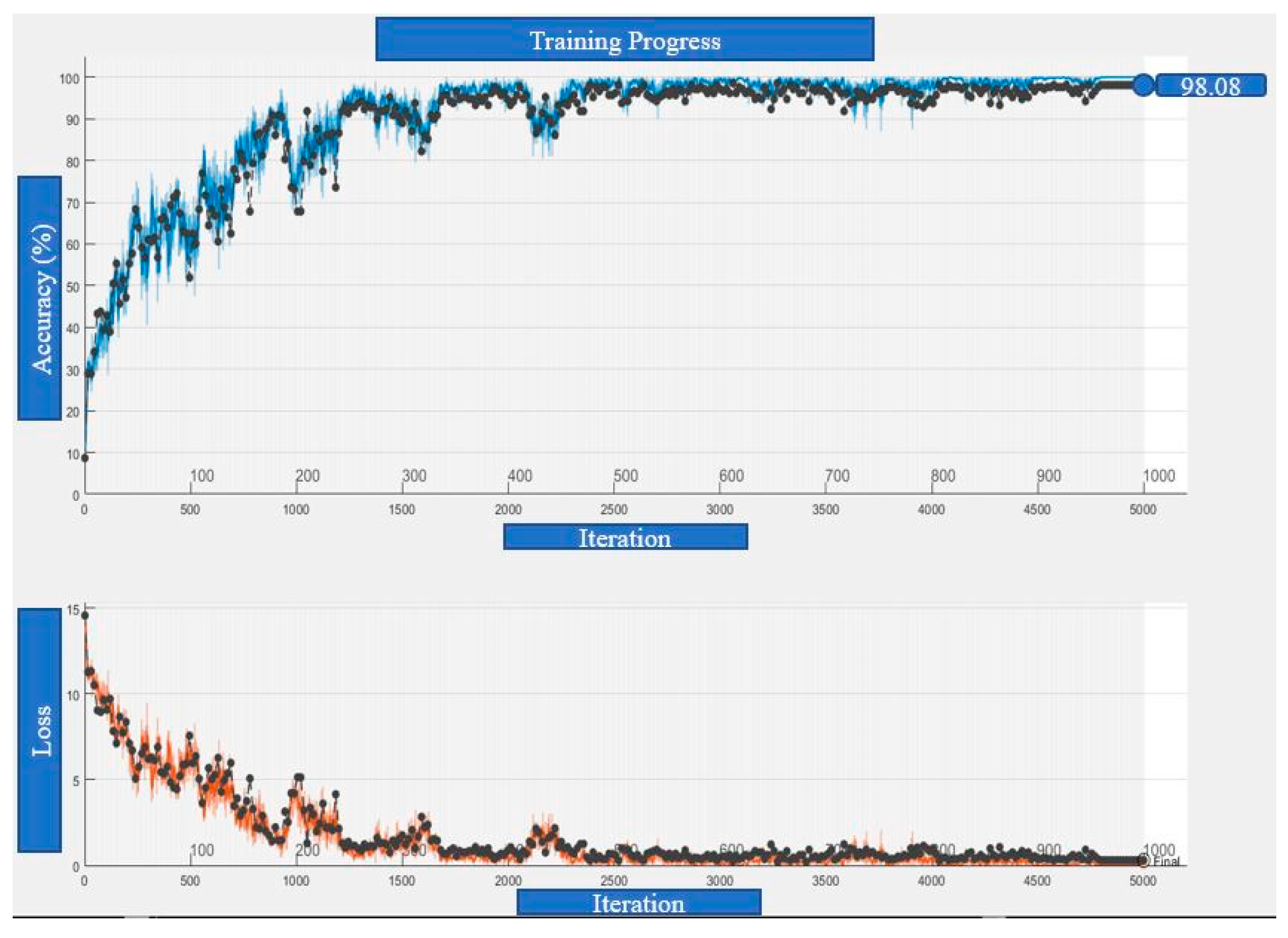
3.3. Convolutional Neural Network

The choice of the deep learning algorithm was based on the use of Convolutional Neural Networks (CNNs) due to the fact that the Gramian Angular Field algorithm encodes time series signals into an image. CNNs are suitable for image recognition and it is possible to use the ConvNet architecture to train a network and use it later to obtain a categorical or numerical label. It is also possible to extract features from a previously trained network and use them to train a linear classifier. Furthermore, it is possible to carry out transfer learning, which consists of retraining the last connected layer of an already existing ConvNet on new data. CNNs are made up of neurons connected to each other by weighted branches; the trainable parameters of the nets are, therefore, always the weight and the bias. However, CNNs make the specific assumption that their input has a precise data structure, such as an image in this case, and this allows them to assume specific properties in their architecture to better elaborate these data. The network used was GoogLeNet [35,36], a 22-layer deep convolutional neural network. The network trained on ImageNet [37] classifies images into 1000 categories of objects and it has an image input size of 224 × 224. To improve the performance of in-depth learning, GoogLeNet uses nine startup modules. A bottleneck approach was used to rebuild the boot module with more non-linearity and fewer parameters. In addition, a maximum pool level was added to summarize the contents of the previous level. All results were concatenated one after the other and given to the next level.

4. Results and Discussions

In Tests A and B, the analyzed data came from a single triaxial accelerometer. Instead, in Test D, the data came from a triaxial accelerometer, a monoaxial and a sound level meter. The first three analyses were not very significant, since the aerodynamic effects were mixed with noise. For this reason, it was difficult to create a correlation between helmet performance and a comfort index.

The last analysis (Test C) returned significant values for the definition of a comfort coefficient. The analysis was no longer with air flow at constant speed, but with a ramp of speed values from 0 to 160 km/h. Five different helmet configurations were tested and colormaps were used to obtain a clearer phenomenon. The images shown below refer to the third helmet analyzed, since, in that configuration, aerodynamic phenomena manifested themselves in a marked manner. The data from the analysis with Support I and Support II were compared to clarify whether the phenomenon was visible in both configurations. As reported in Figure 5, the signals from accelerometers showed two fixed frequencies (one at 27 Hz and one at 33 Hz) considered as external disturbances. Sound level meters and accelerometers, starting from a wind speed of 25 m/s, had a variable frequency component ranging from 75 Hz to 85 Hz. It was clear that the aerodynamic phenomena were present in both configurations; however, the second configuration (Support II) introduced the analysis of the noise components (from 100 Hz to 150 Hz) which made reading the data less clear. For this reason, it was chosen to analyze the configuration with Support I (rigid).

As shown in Figure 6, the correlation between the two measuring instruments can be stated. This led to the choice of examining the sound level data individually. The best helmet and the worst helmet were, therefore, defined and based on the parameters analyzed so far.

In Figure 7, the colormaps relating to the best helmet examined and the worst are represented. From these results, a CNN can be trained with the aim of classifying the remaining helmets examined. All the sensor channels used were, therefore, analyzed individually. The signals were sampled to have a stationary phenomenon within each selected range. The process, in its first phase, started with the creation of the GASF matrices (3.1. Gramian Angular Field) using all the channels of each sensor. The created matrices were superimposed to create the three RGB channels of the image (Figure 8).

The aim was to correlate the aerodynamic related phenomena with the stresses acting on the support. The three GASF matrices chosen to create RGB images (Figure 9) and used to train the CNN were:

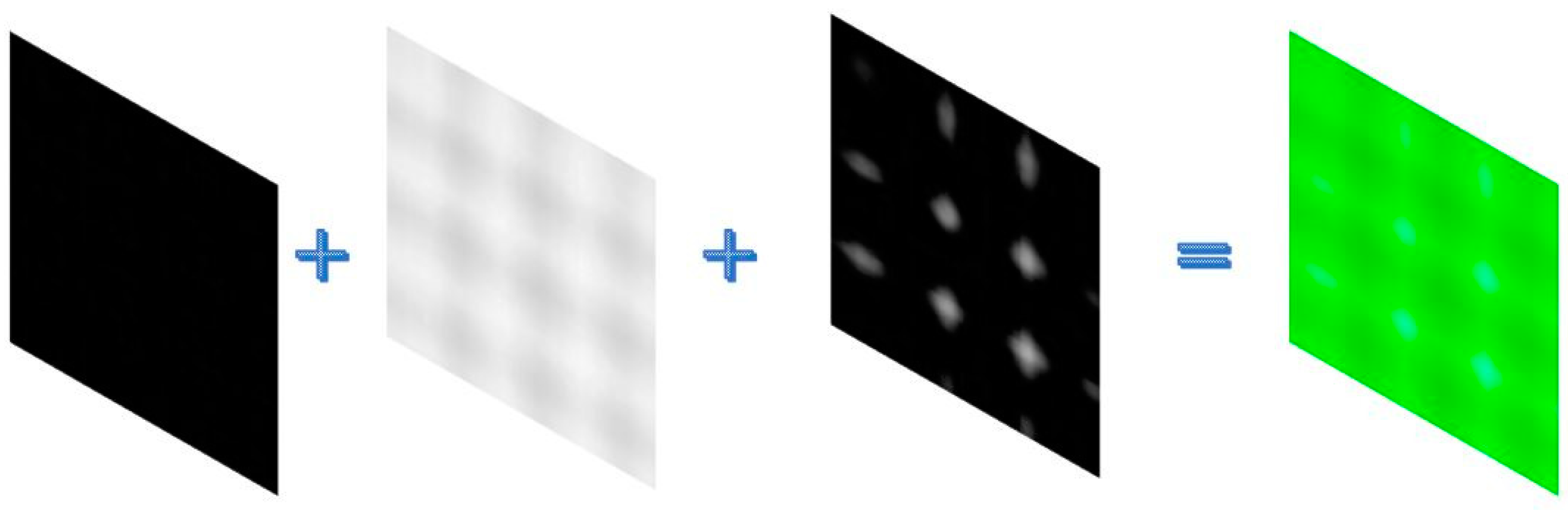
• Red—Moment along the x axis.
• Green—Force along the y axis.
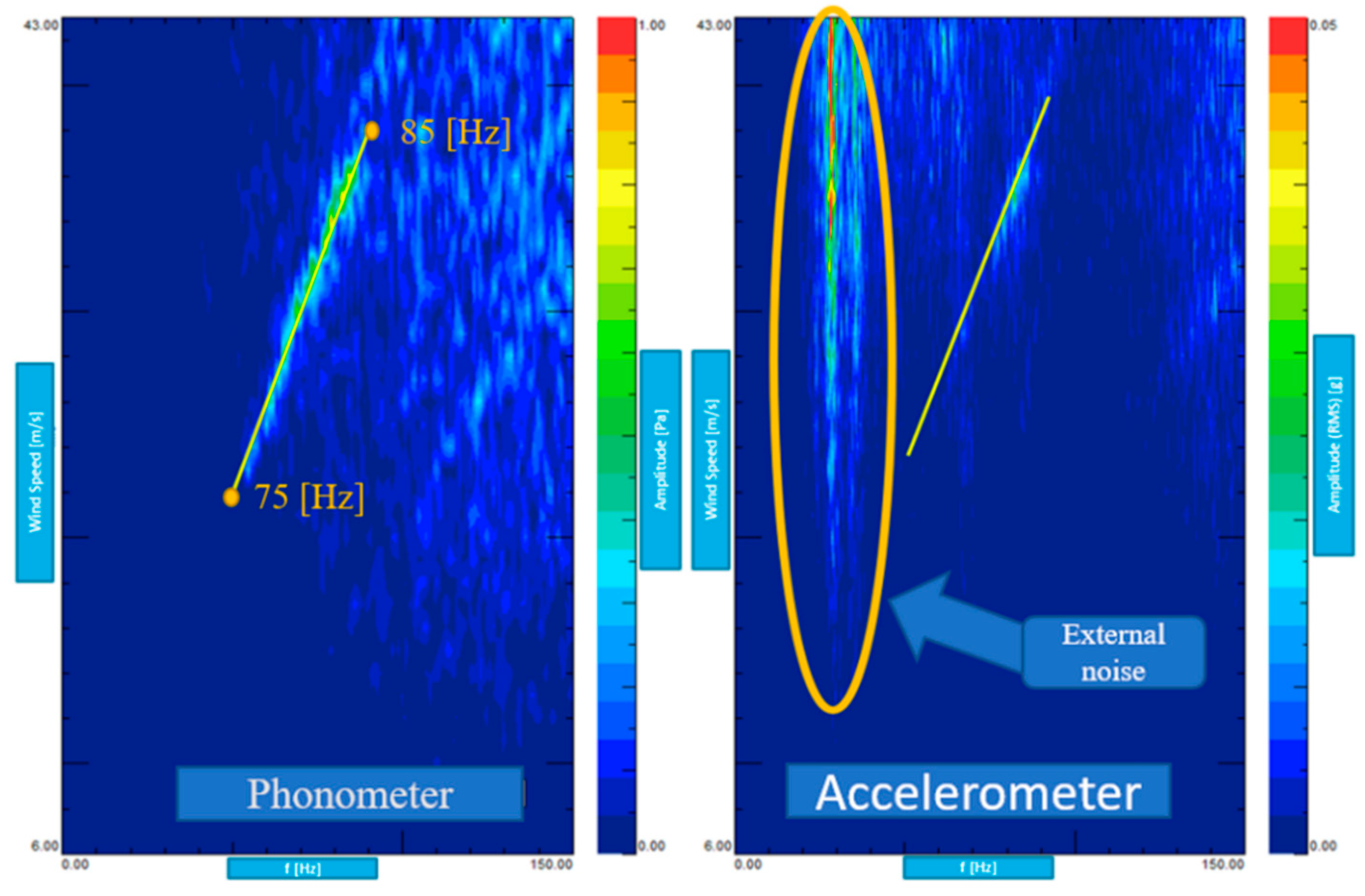
• Blue—Left sound level meter.

These signals were chosen, since:

• The phonometric data are less affected by external noise compared to accelerometers.
• Analyzing the load cells, forces along the y axis and the moments along the x axis present a greater intensity than the other components.

For the creation of the dataset, to simplify the calculation, the images that refer to wind speeds below 25 m/s were not considered, since the aerodynamic phenomena were clearly visible above this threshold. The last step taken into consideration was to give a label to each image created. It was, therefore, decided to group all the data relating to a helmet in folders labelled with the commercial name of the same. At this point, each briefcase had a unique identifier for each helmet. At the upstream of the analysis, the best and worst helmets were labelled. Based on their characteristics (set of images that describe them), the CNN will associate a percentage of similarity of each unlabeled folder (each folder was related to a given helmet), to one of the two helmets. The next step was training the network. The loss was calculated on training and validation and its interpretation was based on how well the model was doing in these two sets; it was the sum of errors performed for each example in training or validation sets. Loss value implied how poorly or well a model behaved after each iteration of optimization. An accuracy metric was used to measure the algorithm’s performance in an interpretable way. The accuracy of a model was usually determined after the model parameters and was calculated in the form of a percentage. It was the measure of how accurate your model’s prediction was compared to the true data (Figure 10).

As shown in Figure 10, after 5000 iterations it was trained to classify helmets. The same managed to identify each data and proceeded to its classification with an accuracy of 98.08%.

Assuming 100% as an index of comfort meant that the tested helmet was equal to the best result of the dataset; an amount of 0%, on the contrary. The results obtained are shown in Figure 11.

Below the line, the starting helmets are shown used to label the rest of the data. The three helmets above the line are, respectively:

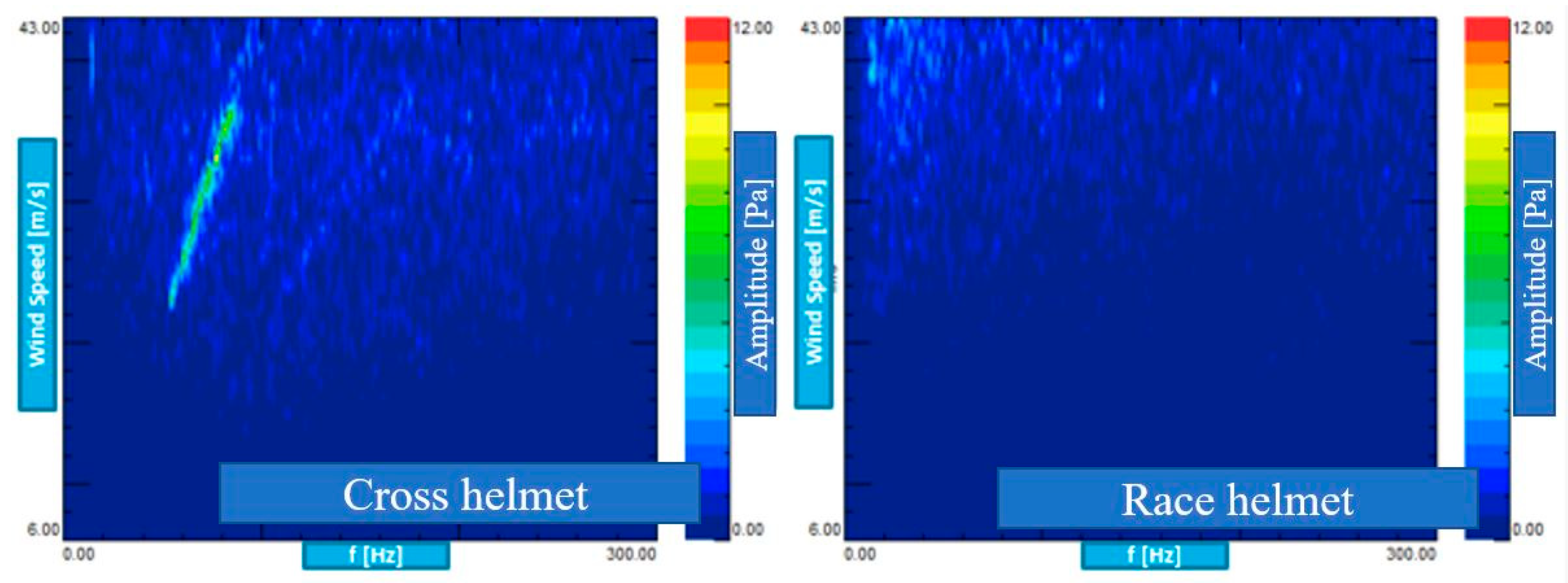
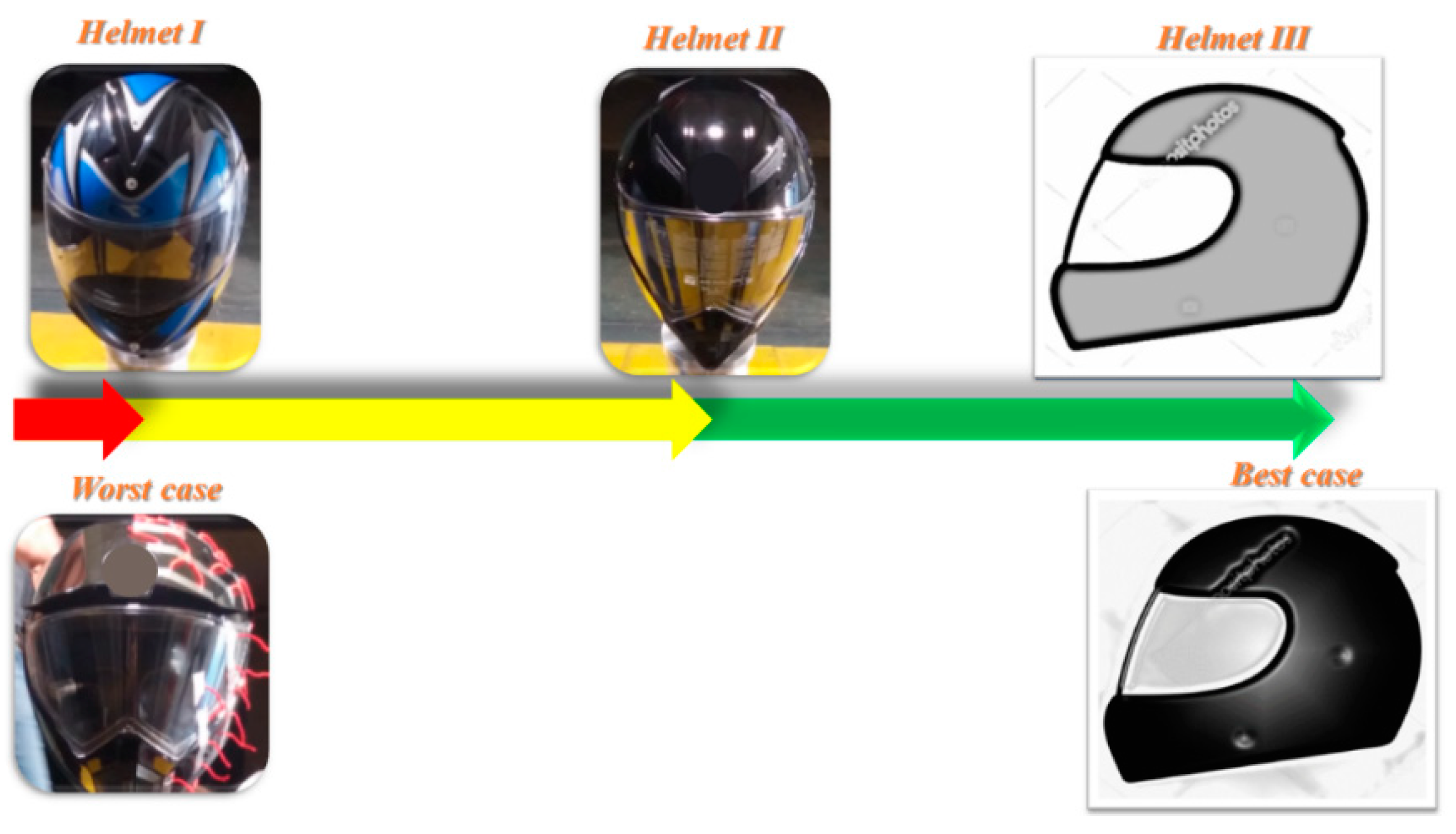
• Helmet I: corresponds to 98.8% to the worst helmet and 0.2% to the best;
• Helmet II: corresponds to 50% to the worst helmet and 50% to the best;
• Helmet III: corresponds to 0.8% for the worst helmet and 98.2% for the best.

5. Conclusions

The aim was to objectify a subjective phenomenon such as comfort. In the first phase, an analysis was performed in the field of frequencies, in order to highlight the aerodynamic phenomena acting on the system, and the disturbances related to the experimental setup. From the analysis conducted, it was found that there was a correlation between the phenomena read by the sound level meters and the accelerometers. It also appeared that the data from the former were less affected by noise. It was discovered that aerodynamic phenomena did not occur at a fixed frequency and, furthermore, below certain wind speeds (25 m/s), all helmets showed the same trend. The configuration with the rigid neck was more significant than the hybrid 3. By identifying the best helmet and the worst, through the use of a CNN, specifically GoogLeNet, it will be possible to obtain an index relating to the aerodynamic characteristics of a given helmet. In conclusion, this type of analysis was the best method to characterize a comfort index.

References

- Al-Dhahebi, A.M.; Junoh, A.K.; Mohamed, Z.; Muhamad, W.Z.A.W. A computational approach for optimizing vehicles’ interior noise and vibration. Int. J. Automot. Mech. Eng. 2017, 14, 4690–4703. [Google Scholar] [CrossRef]
- Yan, L.; Chen, Z.; Zou, Y.; He, X.; Cai, C.; Yu, K.; Zhu, X. Field study of the interior noise and vibration of a metro vehicle running on a viaduct: A case study in Guangzhou. Int. J. Environ. Res. Public Health 2020, 17, 2807. [Google Scholar] [CrossRef] [Green Version]
- Angeletti, M.; Sclafani, L.; Bella, G.; Ubertini, S. The role of CFD on the aerodynamic investigation of motorcycles. SAE Trans. 2003, 112, 1103–1111. [Google Scholar] [CrossRef]
- Scappaticci, L.; Risitano, G.; Battistoni, M.; Grimaldi, C. Drag Optimization of a Sport Motorbike; SAE Technical Paper; SAE International: Warrendale, PA, USA, 2012. [Google Scholar] [CrossRef]
- Mariani, F.; Risi, F.; Bartolini, N.; Castellani, F.; Scappaticci, L. Spoilers Optimization to Reduce the Induced Stresses on a Racing Helmet; SAE Technical Paper; SAE International: Warrendale, PA, USA, 2016. [Google Scholar] [CrossRef]
- Harris, C.M.; Bert, C.W. Shock and vibration handbook. J. Appl. Mech. 1989, 56, 487. [Google Scholar] [CrossRef] [Green Version]
- Tamer, A.; Zanoni, A.; Cocco, A.; Masarati, P. A numerical study of vibration-induced instrument reading capability degradation in helicopter pilots. CEAS Aeronaut. J. 2021, 12, 427–440. [Google Scholar] [CrossRef]
- Griffin, M.J.; Erdreich, J. Handbook of human vibration. J. Acoust. Soc. Am. 1991, 90, 2213. [Google Scholar] [CrossRef]
- Griffin, M.J. Vibration and human responses. In Handbook of Human Vibration; Academic Press: Cambridge, MA, USA, 1990. [Google Scholar]
- Hulshof, C.; Van Zanten, B.V. Whole-body vibration and low-back pain—A review of epidemiologic studies. Int. Arch. Occup. Environ. Health 1987, 59, 205–220. [Google Scholar] [CrossRef]
- Fairley, T.E. Predicting the discomfort caused by tractor vibration. Ergonomics 1995, 38, 2091–2106. [Google Scholar] [CrossRef]
- Gillespie, T.D.; Sayers, M.W.; Segel, L. Calibration of Response-Type Road Roughness Measuring Systems; TRB, National Research Council: Washington, DC, USA, 1980. [Google Scholar]
- Crocker, M.J.; Ramakrishnan, R. Handbook of noise and vibration control. Noise Control. Eng. J. 2008, 56, 218. [Google Scholar] [CrossRef]
- Tamer, A.; Muscarello, V.; Quaranta, G.; Masarati, P. Cabebin layout optimization for vibration hazard reduction in helicopter emergency medical service. Aerospace 2020, 7, 59. [Google Scholar] [CrossRef]
- Tamer, A.; Muscarello, V.; Masarati, P.; Quaranta, G. Evaluation of vibration reduction devices for helicopter ride quality improvement. Aerosp. Sci. Technol. 2019, 95, 105456. [Google Scholar] [CrossRef]
- Measuring Vibration. Available online: https://www.bksv.com/en/knowledge/blog/vibration/measuring-vibration (accessed on 1 August 2021).
- Mechanical Vibration and Shock—Evaluation of Human Exposure to Whole-Body Vibration; ANSI: New York, NY, USA, 2001.
- Von Gierke, H.E.; Brammer, A.J. Harris’ Shock and Vibration Handbook; Mcgraw-Hill: New York, NY, USA, 2007. [Google Scholar]
- Licht, T.R.; Zaveri, K. Vibration and shock measurement. Meas. Control. 1982, 15, 9–13. [Google Scholar] [CrossRef]
- Berthoz, A. The Brain’s Sense of Movement; Harvard University Press: Cambridge, MA, USA, 2000. [Google Scholar]
- Pennestri, E.; Valentini, P.P.; Vita, L. Comfort analysis of car occupants: Comparison between multibody and finite element models. Int. J. Veh. Syst. Model. Test. 2005, 1, 68–78. [Google Scholar] [CrossRef] [Green Version]
- De Lange, R.; Van Rooij, L.; Mooi, H.; Wismans, J. Objective Biofidelity Rating of a Numerical Human Occupant Model in Frontal to Lateral Impact; SAE Technical Paper; SAE International: Warrendale, PA, USA, 2005. [Google Scholar] [CrossRef]
- Dieckmann, D. A Study of the influence of vibration on man. Ergonomics 1958, 1, 347–355. [Google Scholar] [CrossRef]
- Coermann, R.R.; Ziegenruecker, G.H.; Wittwer, A.L.; Von Gierke, H.E. The passive dynamic mechanical properties of the human thorax-abdomen system and of the whole body system. Aerosp. Med. 1960, 31, 443–455. [Google Scholar] [PubMed]
- Magid, E.B.; Coermann, R.R.; Ziegenruecker, G.H. Human tolerance to whole body sinusoidal vibration. Short-time, one-minute and three-minute studies. Aerosp. Med. 1960, 31, 915–924. [Google Scholar] [PubMed]
- Chaffin, D.B. A computerized biomechanical model—Development of and use in studying gross body actions. J. Biomech. 1969, 2, 429–441. [Google Scholar] [CrossRef] [Green Version]
- Gruver, W.A.; Ayoub, M.A.; Muth, M.B. A model for optimal evaluation of manual lifting tasks. J. Saf. Res. 1979, 11, 61–71. [Google Scholar]
- Kane, T.R.; Scher, M.P. Human self-rotation by means of limb movements. J. Biomech. 1970, 39–49. [Google Scholar] [CrossRef]
- Passerello, C.; Huston, R. Human attitude control. J. Biomech. 1971, 4, 95–102. [Google Scholar] [CrossRef]
- ISO. International Standard ISO 2631-4; ISO—International Organization for Standardization: Geneva, Switzerland, 2001. [Google Scholar]
- ISO. ISO 2631-5:2018 International Standard Mechanical Vibration—Evaluation; ISO: Geneva, Switzerland, 2018. [Google Scholar]
- ISO-International Organization for Standardization. ISO 2631-1: Mechanical Vibration and Shock-Evaluation of Human Exposure to Whole-Body Vibration-Part 1: General Requirements; ISO-International Organization for Standardization: Geneva, Switzerland, 2010. [Google Scholar]
- Wang, Z.; Oates, T. Imaging time-series to improve classification and imputation. In Proceedings of the Twenty-Fourth International Joint Conference on Artificial Intelligence, Buenos Aires, Argentina, 25–31 July 2015. [Google Scholar]
- Dengwen, Z. An edge-directed bicubic interpolation algorithm. In Proceedings of the Twenty-Fourth International Joint Conference on Artificial Intelligence, Yantai, China, 16–18 October 2010; Volume 3, pp. 1186–1189. [Google Scholar] [CrossRef]
- Szegedy, C.; Liu, W.; Jia, Y.; Sermanet, P.; Reed, S.; Anguelov, D.; Erhan, D.; Vanhoucke, V.; Rabinovich, A. Going deeper with convolutions. In Proceedings of the IEEE Conference on Computer Vision and Pattern Recognition, Boston, MA, USA, 7–12 June 2015. [Google Scholar] [CrossRef] [Green Version]
- Zeng, G.; He, Y.; Yu, Z.; Yang, X.; Yang, R.; Zhang, L. InceptionNet/googlenet-going deeper with convolutions. Cvpr 2016, 91, 2322–2330. [Google Scholar]
- Krizhevsky, A.; Sutskever, I.; Hinton, G.E. ImageNet classification with deep convolutional neural networks. Commun. ACM 2017, 60, 84–90. [Google Scholar] [CrossRef]