A Robust Indicator Mean-Based Method for Estimating Generalizability Theory Absolute Error and Related Dependability Indices within Structural Equation Modeling Frameworks

Abstract

In this study, we introduce a novel and robust approach for computing Generalizability Theory (GT) absolute error and related dependability indices using indicator intercepts that represent observed means within structural equation models (SEMs). We demonstrate the applicability of our method using one-, two-, and three-facet designs with self-report measures having varying numbers of scale points. Results for the indicator mean-based method align well with those obtained from the GENOVA and R gtheory packages for doing conventional GT analyses and improve upon previously suggested methods for deriving absolute error and corresponding dependability indices from SEMs when analyzing three-facet designs. We further extend our approach to derive Monte Carlo confidence intervals for all key indices and to incorporate estimation procedures that correct for scale coarseness effects commonly observed when analyzing binary or ordinal data.

1. Introduction

Generalizability theory (GT; [1,2,3,4]) offers an effective framework for accounting for multiple sources of measurement error when assessing the accuracy of measurement data and subsequently using that information to evaluate and improve assessment procedures. Such techniques have recently been applied to advantage in such diverse fields as education [5,6,7,8,9,10,11,12,13], psychology [14,15,16,17], business [18,19,20,21], medicine/health sciences [22,23,24,25,26,27,28,29], psychophysiology [30,31,32], athletic training [33,34,35], and many others. Although GT designs have traditionally been analyzed using analysis of variance (ANOVA) procedures, they also can be analyzed using linear mixed-effect [36,37] and structural equation models (SEMs; [14,37,38,39,40,41,42,43,44,45,46,47,48,49,50,51,52,53,54]).

Using SEMs to conduct GT analyses has many advantages including use of alternative estimation procedures to correct for scale coarseness effects (diagonally weighted least squares, paired maximum likelihood, etc.; [14,38,42,44,45,46,49]), derivation of Monte Carlo confidence intervals for key indices of interest [14,44,46,47,50,51,55,56], partitioning of variance at both total score and individual item levels [46,47,48,49], and extensions to multivariate [37,46,47,50,51] and bifactor model GT designs [46,50,52,53,54]. These advantages stem in part from the inherent capabilities of SEM programs to tailor factor loadings, variances, residuals, intercepts, and thresholds to specific needs and contexts of assessment.

GT can be used with both objectively and subjectively scored measures to yield indices reflecting the accuracy of scores used for either norm- or criterion-referencing purposes. However, initial uses of SEMs for conducting GT analyses were limited to derivation of variance components and related generalizability (G) coefficients for norm-referencing purposes that only reflected relative rather than absolute differences in scores (see, e.g., [38,39,40,41,42,43]). To address this limitation within one- and two-facet GT designs, Jorgensen [44] devised methods for estimating variance components reflecting absolute differences in scores that together with variance components for relative differences can be used to derive dependability coefficients for making criterion-referenced decisions. When using Jorgensen’s method, variance components for absolute differences in scores are obtained indirectly from SEMs by placing constraints on mean structure parameters. In the study reported here, we propose an alternative method for deriving variance components for absolute differences in scores based on factor indicator means that can be extended beyond two measurement facets. We compare results for the indicator mean-based method to those obtained using the standalone ANOVA-based GT package GENOVA [57], the gtheory package in R [58,59], and Jorgensen’s [44] SEM-based method applied within the lavaan package in R [60,61] when analyzing one-, two-, and three-facet designs. Results are based on multi-occasion data obtained from the Music Self-Perception Inventory (MUSPI; [62,63,64]), with designs having two, four, or eight scale points for all items. We further extend the overall SEM GT analyses to allow for derivation of Monte Carlo confidence intervals for key parameters and corrections for possible scale coarseness effects resulting from limited numbers of response options and/or unequal intervals between those options.

2. Background

2.1. Generalizability Theory

GT subdivides measurement or generalization error into distinct facets reflecting variations in scores for items, occasions, raters, and other relevant entities. Universe scores in GT are analogous to true scores in classical test theory and to communality in factor analysis. However, in contrast to these other contexts, universe scores in GT represent estimated average scores that individuals would receive across all observable facet conditions within the assessment domain(s) of interest. In its broadest sense, an observed score in GT represents universe score plus “absolute” or total error, with absolute error representing the overall deviation of an individual’s observed score from his or her universe score. Absolute error encompasses all sources of error, including those that affect the consistency of rankings (relative error) as well as differences in the absolute magnitudes of scores. More specifically, relative error variance is the sum of interaction effects that involve persons (or objects of measurement), whereas absolute error is the sum of all facet effects that include interactions between person and facet effects as well as main and interaction effects for the facets themselves.

Estimates of variance components for universe scores and measurement errors allow for computation of several GT-based reliability-like indices. Generalizability (G or Eρ²) and dependability (D or ϕ) coefficients, respectively, underpin decision-making processes tailored to norm-referenced and criterion-referenced decisions. A G coefficient (Equation (1)) is computed as the ratio of universe score variance over the combined variances for universe score and relative error, rendering it particularly useful when representing relative differences in observed scores across individuals. This is especially pertinent in large-scale assessments where the priority is to rank individuals according to their relative performance levels. In contrast, a D coefficient encompasses total or absolute error rather than just relative error, thereby providing a more inclusive and comprehensive assessment of measurement precision. D coefficients fall into two categories, with the “global D coefficient” (Equation (2)) providing a summary index of dependability across all scores derived from the assessment procedure, and the “cut-score-specific D coefficient” (Equation (3)) reflecting dependability or random classification agreement at a predetermined level of performance or endorsement represented by a cut score [65,66,67].

$$\mathrm{G} \mathrm{coefficient}=\frac{\mathrm{U}\mathrm{n}\mathrm{i}\mathrm{v}\mathrm{e}\mathrm{r}\mathrm{s}\mathrm{e} \mathrm{s}\mathrm{c}\mathrm{o}\mathrm{r}\mathrm{e} \mathrm{v}\mathrm{a}\mathrm{r}\mathrm{i}\mathrm{a}\mathrm{n}\mathrm{c}\mathrm{e}}{\mathrm{U}\mathrm{n}\mathrm{i}\mathrm{v}\mathrm{e}\mathrm{r}\mathrm{s}\mathrm{e} \mathrm{s}\mathrm{c}\mathrm{o}\mathrm{r}\mathrm{e} \mathrm{v}\mathrm{a}\mathrm{r}\mathrm{i}\mathrm{a}\mathrm{n}\mathrm{c}\mathrm{e}+\mathrm{R}\mathrm{e}\mathrm{l}\mathrm{a}\mathrm{t}\mathrm{i}\mathrm{v}\mathrm{e} \mathrm{e}\mathrm{r}\mathrm{r}\mathrm{o}\mathrm{r} \mathrm{v}\mathrm{a}\mathrm{r}\mathrm{i}\mathrm{a}\mathrm{n}\mathrm{c}\mathrm{e}} .$$

(1)

$$\mathrm{Global} \mathrm{D} \mathrm{coefficient}=\frac{\mathrm{U}\mathrm{n}\mathrm{i}\mathrm{v}\mathrm{e}\mathrm{r}\mathrm{s}\mathrm{e} \mathrm{s}\mathrm{c}\mathrm{o}\mathrm{r}\mathrm{e} \mathrm{v}\mathrm{a}\mathrm{r}\mathrm{i}\mathrm{a}\mathrm{n}\mathrm{c}\mathrm{e}}{\mathrm{U}\mathrm{n}\mathrm{i}\mathrm{v}\mathrm{e}\mathrm{r}\mathrm{s}\mathrm{e} \mathrm{s}\mathrm{c}\mathrm{o}\mathrm{r}\mathrm{e} \mathrm{v}\mathrm{a}\mathrm{r}\mathrm{i}\mathrm{a}\mathrm{n}\mathrm{c}\mathrm{e}+\mathrm{A}\mathrm{b}\mathrm{s}\mathrm{o}\mathrm{l}\mathrm{u}\mathrm{t}\mathrm{e} \mathrm{e}\mathrm{r}\mathrm{r}\mathrm{o}\mathrm{r} \mathrm{v}\mathrm{a}\mathrm{r}\mathrm{i}\mathrm{a}\mathrm{n}\mathrm{c}\mathrm{e}} .$$

(2)

$$\mathrm{Cut}\text{-}\mathrm{score}\text{-}\mathrm{specific} \mathrm{D} \mathrm{coefficient}=\frac{\mathrm{U}\mathrm{n}\mathrm{i}\mathrm{v}\mathrm{e}\mathrm{r}\mathrm{s}\mathrm{e} \mathrm{s}\mathrm{c}\mathrm{o}\mathrm{r}\mathrm{e} \mathrm{v}\mathrm{a}\mathrm{r}\mathrm{i}\mathrm{a}\mathrm{n}\mathrm{c}\mathrm{e}+{({\mu }_Y-cut score)}^2}{\mathrm{U}\mathrm{n}\mathrm{i}\mathrm{v}\mathrm{e}\mathrm{r}\mathrm{s}\mathrm{e} \mathrm{s}\mathrm{c}\mathrm{o}\mathrm{r}\mathrm{e} \mathrm{v}\mathrm{a}\mathrm{r}\mathrm{i}\mathrm{a}\mathrm{n}\mathrm{c}\mathrm{e}+{({\mu }_Y-cut score)}^2+\mathrm{A}\mathrm{b}\mathrm{s}\mathrm{o}\mathrm{l}\mathrm{u}\mathrm{t}\mathrm{e} \mathrm{e}\mathrm{r}\mathrm{r}\mathrm{o}\mathrm{r} \mathrm{v}\mathrm{a}\mathrm{r}\mathrm{i}\mathrm{a}\mathrm{n}\mathrm{c}\mathrm{e}} .$$

(3)

2.2. Estimation of Universe Scores and Relative Error Using SEMs

In the study reported here, we will use SEMs to represent random effects GT designs based on responses to the adult form of the Music Self-Perception Inventory (MUSPI; [62,63,64]) and the measurement facets items, occasions, and skills. More specifically, we will consider the following three random effects designs: persons × items (pi), persons × items × occasions (pio), and persons × items × occasions × skills (pios). Partitioning of variance at the individual score level within those designs is shown in Equations (4)–(6).

$$p\times i (pi) \mathrm{design}:{\sigma }_{Y_{pi}}^2= {\sigma }_p^2 + {\sigma }_{pi,e}^2+ {\sigma }_i^2 ,$$

(4)

$$p\times i\times o (pio) \mathrm{design}:{ \sigma }_{Y_{pio}}^2= {\sigma }_p^2 + {\sigma }_{pi}^2 + {\sigma }_{po}^2 + {\sigma }_{pio,e}^2+ {\sigma }_i^2 + {\sigma }_o^2 + {\sigma }_{io}^2 ,$$

(5)

$$\begin{array}{l}p\times i\times o\times s (pios) \mathrm{design}:{ \sigma }_{Y_{pios}}^2= {\sigma }_p^2 + {\sigma }_{pi}^2 + {\sigma }_{po}^2 + {\sigma }_{ps}^2+ {\sigma }_{pio}^2 + {\sigma }_{pis}^2 + {\sigma }_{pos}^2+ {\sigma }_{pios,e}^2\\ \hspace{1em}\hspace{1em}\hspace{1em}\hspace{1em}\hspace{1em}\hspace{1em}\hspace{1em}\hspace{1em}\hspace{1em}\hspace{1em}\hspace{1em}\hspace{1em} +{\sigma }_i^2 + {\sigma }_o^2 + {\sigma }_s^2 + {\sigma }_{io}^2 + {\sigma }_{is}^2 + {\sigma }_{os}^2+ {\sigma }_{ios}^2. \end{array}$$

(6)

The Y scores in Equations (4)–(6) are not aggregated. In Equation (4), they represent individual item scores; in Equation (5), they represent individual combinations of item and occasion scores; and in Equation (6), they represent individual combinations of item, occasion, and skill scores. Variance components on the right side of these equations involving interactions with persons (p) reflect relative differences in scores, whereas those not involving persons reflect absolute differences in mean scores. When “,e” is included within the subscript for a relative error term, it indicates that any remaining relative residual error in the design is also included in that term. As evident from Equations (4)–(6), the number of variance components reflecting both relative and absolute differences in scores noticeably increases as the number of measurement facets increase, which, in turn, adds greater layers of complexity when analyzing GT designs.

The three diagrams in Figure 1, respectively, represent all possible variance components included in random-facet pi, pio, and pios designs. Within the figure, the circles for a given diagram collectively represent overall observed score variance (${\sigma }_Y^2)$, ${\sigma }_p^2$ represents universe score variance, variance terms that include interactions between persons and measurement facets represent relative differences in scores, and variance terms for main and interaction effects involving facets alone represent absolute differences in mean scores. When using SEMs to analyze the three designs described above, variance components for persons and sources of relative measurement error are estimated directly, whereas those for absolute differences in scores are estimated indirectly using additional formulas that we later provide.

Within the SEMs for the pi, pio, and pios designs, universe or person scores are represented by a single factor that has unit loadings on all observed variables (or indicators) to define explained variance (${\sigma }_p^2$) shared across all observations. The interaction term that includes person scores and all facets within a given design is represented as a common residual or uniqueness across all indicators. For example, in a single-facet, pi design with four items, four indicators are used to represent person scores, and the variance for the person factor (${\sigma }_p^2$) and common residual (${\sigma }_{pi,e}^2$) are estimated.

Designs involving more than one facet require additional factors to account for interactions of persons with all possible combinations of relevant measurement facets. In a two-facet, pio design with four items and two occasions, there are eight (4 × 2) indicators representing Items 1 to 4 across Occasions 1 and 2. The person factor again is linked to all indicators with unit loadings, and its variance (${\sigma }_p^2$) is estimated. Additional factors are included for each item across all occasions and for each occasion across all items, with all loadings again set equal to one. Variances for all item factors are set equal, and this common variance represents an estimate of ${\sigma }_{pi}^2$. Similarly, variances for all occasion factors are set equal, and that common variance represents as estimate of ${\sigma }_{po}^2$. Finally, uniquenesses for all indicators are set equal, and this common uniqueness provides an estimate of ${\sigma }_{pio,e}^2$. In all, four variances are estimated to represent person scores (${\sigma }_p^2$) and three sources of relative error variance (${\sigma }_{pi}^2, {\sigma }_{po}^2, {\sigma }_{pio,e}^2$).

In a three-facet, pios design with four items, two occasions, and three skills, there are 24 (4 × 2 × 3) indicators in total. In this design, eight variances would be directly estimated to represent relative differences in scores, with one for persons (${\sigma }_p^2$), three for the two-way interactions involving persons (${\sigma }_{pi}^2,{\sigma }_{po}^2,{\sigma }_{ps}^2)$, three for the three-way interactions involving persons $({\sigma }_{pio}^2,{\sigma }_{pis}^2,{\sigma }_{pos}^2)$, and one for the four-way interaction involving persons (${\sigma }_{pios,e}^2$). As in the other designs, the person factor is linked to all indicators with unit loadings, and its variance (${\sigma }_p^2$) is estimated. For the two-way interactions, there would be a separate factor for each targeted facet linked to all combinations of the other two facets. For example, if items represent the targeted facet, there would be a separate factor for each item linked to all combinations of occasions and skills (entailing 2 × 3 = 6 indicators here), and the variances for the four item factors would be set equal to estimate ${\sigma }_{pi}^2$. This same process would be repeated separately for occasions and skills to estimate ${\sigma }_{po}^2$ and ${\sigma }_{ps}^2$.

For the three-way interactions, there would be a separate factor for each combination of the two targeted facets linked to all conditions for the remaining facet. For example, if items and occasions are the targeted facets, there would be a separate factor for each combination of items and occasions (4 × 2 = 8 factors here) linked to all skills, and the variances for the eight relevant factors would be set equal to estimate ${\sigma }_{pio}^2$. This process would be repeated for the remaining two possible pairs of targeted facets (items & skills; occasions & skills) to estimate ${\sigma }_{pis}^2$ and ${\sigma }_{pos}^2.$ Finally, uniquenesses for all 24 indicators are set equal, and this common uniqueness is used to estimate ${\sigma }_{pios,e}^2$. In all, eight variances are estimated within this three-facet design to represent person scores (${\sigma }_p^2$) and the seven sources of relative error variance (${\sigma }_{pi}^2, {\sigma }_{po}^2, {\sigma }_{ps}^2{,\sigma }_{pio}^2, {\sigma }_{pis}^2,{\sigma }_{pos}^2, {\sigma }_{pios,e}^2$). More detailed information about setting constraints for all SEMs illustrated in this article is provided in our online Supplementary Material. Although the complexity of the pios design with its numerous overlapping factors renders it impractical to represent within a simple factor model diagram, examples of such diagrams for pi and pio designs with the same constraints described here can be found in [14,68].

2.3. Overview of Absolute Error Estimation within SEMs

The preceding methodology for estimating variance components for universe score and relative error within SEMs was first described by Marcoulides [39] and Raykov and Marcoulides [41] for one- and two-facet designs and more recently revisited and expanded upon by others (see, e.g., [42,43,45,48]). Subsequently, Jorgensen [44] introduced an approach to estimate absolute error within SEMs using the same one- and two-facet SEM designs described in previous studies.

When using both Jorgensen’s and our approaches, variance components reflecting absolute differences in scores are derived using ANOVA-like formulas that ultimately represent estimates of average squared differences of facet condition means from the grand mean across all relevant facet conditions with or without controlling for the effects of other facets. With Jorgensen’s approach, the global person factor mean will equal the grand mean (μ) across all measurement conditions, and other factor means will equal mean deviation scores. In contrast, our approach relies exclusively on indicator intercepts that represent means for all possible combinations of facet conditions. In sections to follow, we describe how both methods are used to estimate variance components reflecting absolute differences in scores within pi, pio, and pios GT designs. Due to its simplicity and more transparent relationships with traditional ANOVA formulas, we begin by describing our indicator mean-based method first, and then turn to Jorgensen’s approach.

2.4. The Indicator Mean-Based Method for Estimating Absolute Error Indices

persons × items (pi) designs. As noted above, our method is based solely on the intercepts for all indicators within the relevant SEM and requires no additional constraints other than those already described. In the pi design, the variance component ${\sigma }_i^2$ represents the deviation of each item’s mean from the grand mean. If item means are expressed as intercepts for each observed variable (${\beta }_i$), the estimated grand mean μ will equal the sum of all intercepts in the model divided by the number of items (see Equation (7)).

$$grand \widehat{\mu }=\frac{\sum _{i=1}^{n_i}{\widehat{\beta }}_i}{n_i} ,$$

(7)

where ${ n}_i=\mathrm{t}\mathrm{h}\mathrm{e} \mathrm{n}\mathrm{u}\mathrm{m}\mathrm{b}\mathrm{e}\mathrm{r} \mathrm{o}\mathrm{f} \mathrm{i}\mathrm{t}\mathrm{e}\mathrm{m}\mathrm{s}, {\mathrm{a}\mathrm{n}\mathrm{d} \widehat{\beta }}_{\mathrm{i}} = \mathrm{i}\mathrm{n}\mathrm{t}\mathrm{e}\mathrm{r}\mathrm{c}\mathrm{e}\mathrm{p}\mathrm{t} \mathrm{o}\mathrm{f} i_{th} \mathrm{i}\mathrm{t}\mathrm{e}\mathrm{m}.$

The variance component for items (${\sigma }_i^2$) then can be estimated by summing the squared differences between each mean (or intercept) for items and the grand mean, and then dividing by the number of items minus one (see Equation (8)).

$${\widehat{\sigma }}_i^2=\frac{\sum _{i=1}^{n_i}{\left({\widehat{\beta }}_i-grand \widehat{\mu }\right)}^2}{n_i-1}.$$

(8)

persons × items × occasions (pio) designs. In a two-facet, pio design, the estimated grand mean again is the average of intercepts across all indicators as shown in Equation (9):

$$grand \widehat{\mu }=\frac{\sum _{i=1,o=1}^{{i=n_i,o=n}_o}{\widehat{\beta }}_{io}}{n_i\times n_o} ,$$

(9)

where $n_i=\mathrm{t}\mathrm{h}\mathrm{e} \mathrm{n}\mathrm{u}\mathrm{m}\mathrm{b}\mathrm{e}\mathrm{r} \mathrm{o}\mathrm{f} \mathrm{i}\mathrm{t}\mathrm{e}\mathrm{m}\mathrm{s},$ $n_o=\mathrm{t}\mathrm{h}\mathrm{e} \mathrm{n}\mathrm{u}\mathrm{m}\mathrm{b}\mathrm{e}\mathrm{r} \mathrm{o}\mathrm{f} \mathrm{o}\mathrm{c}\mathrm{c}\mathrm{a}\mathrm{s}\mathrm{i}\mathrm{o}\mathrm{n}\mathrm{s},$ $\mathrm{a}\mathrm{n}\mathrm{d} {\widehat{\beta }}_{io} = \mathrm{i}\mathrm{n}\mathrm{t}\mathrm{e}\mathrm{r}\mathrm{c}\mathrm{e}\mathrm{p}\mathrm{t} \mathrm{o}\mathrm{f} i_{th} \mathrm{i}\mathrm{t}\mathrm{e}\mathrm{m} \mathrm{o}\mathrm{n} \mathrm{t}\mathrm{h}\mathrm{e} o_{th} \mathrm{o}\mathrm{c}\mathrm{c}\mathrm{a}\mathrm{s}\mathrm{i}\mathrm{o}\mathrm{n}.$

The mean for each item is derived by averaging the intercepts for the given item across occasions (see Equation (10)).

$${\widehat{\mu }}_i=\frac{\sum _{o=1}^{n_o}{\widehat{\beta }}_{io}}{n_o}.$$

(10)

As in the pi design, the variance component for items (${\sigma }_i^2$) then can be estimated by summing the squared differences between each item mean and the grand mean and dividing by the number of items minus one (see Equation (11)). This equation parallels Equation (8) except that item means are averaged across occasions, and the grand mean is based on Equation (9) rather than Equation (7).

$${\widehat{\sigma }}_i^2=\frac{\sum _{i=1}^{n_i}{\left({\widehat{\mu }}_i-grand \widehat{\mu }\right)}^2}{n_i-1}.$$

(11)

The variance component for occasions (${\sigma }_o^2$) would be estimated in a similar fashion. The mean for each occasion would be derived by averaging the intercepts for the given occasion across items (see Equation (12)) and the squared differences between each occasion mean and the grand mean would be summed and dividing by the number of occasions minus one (see Equation (13)).

$${\widehat{\mu }}_o=\frac{\sum _{i=1}^{n_i}{\widehat{\beta }}_{io}}{n_i}.$$

(12)

$${\widehat{\sigma }}_o^2=\frac{\sum _{o=1}^{n_o}{\left({\widehat{\mu }}_o-grand \widehat{\mu }\right)}^2}{n_o-1}.$$

(13)

Finally, the variance component for the items × occasions interaction (${\sigma }_{io}^2$) represents the extent to which each combination of item and occasion, on average, deviates from the grand mean after taking the item and occasion main effects into account, as shown in Equation (14).

$${\widehat{\sigma }}_{io}^2=\frac{\sum _{i=1,o=1}^{{i=n}_i,o=n_o}{\left({\widehat{\beta }}_{io}-{\widehat{\mu }}_i-{\widehat{\mu }}_o+grand \widehat{\mu }\right)}^2}{(n_i\times n_o)-1}.$$

(14)

persons × items × occasions × skills (pios) designs. For a three-facet, pios design, the estimated grand mean again is the average of intercepts across all indicators as shown in Equation (15):

$$grand \widehat{\mu }=\frac{\sum _{i=1,\mathrm{o}=1,\mathrm{s}=1}^{{n=n}_i,{o=n}_o,{s=n}_s}{\widehat{\beta }}_{ios}}{n_i\times n_o\times n_s} ,$$

(15)

where $n_i=\mathrm{t}\mathrm{h}\mathrm{e} \mathrm{n}\mathrm{u}\mathrm{m}\mathrm{b}\mathrm{e}\mathrm{r} \mathrm{o}\mathrm{f} \mathrm{i}\mathrm{t}\mathrm{e}\mathrm{m}\mathrm{s},$ $n_o=\mathrm{t}\mathrm{h}\mathrm{e} \mathrm{n}\mathrm{u}\mathrm{m}\mathrm{b}\mathrm{e}\mathrm{r} \mathrm{o}\mathrm{f} \mathrm{o}\mathrm{c}\mathrm{c}\mathrm{a}\mathrm{s}\mathrm{i}\mathrm{o}\mathrm{n}\mathrm{s},$ ${ n}_s=\mathrm{t}\mathrm{h}\mathrm{e} \mathrm{n}\mathrm{u}\mathrm{m}\mathrm{b}\mathrm{e}\mathrm{r} \mathrm{o}\mathrm{f} \mathrm{s}\mathrm{k}\mathrm{i}\mathrm{l}\mathrm{l}\mathrm{s},$ $\mathrm{a}\mathrm{n}\mathrm{d} {\widehat{\beta }}_{ios}=\mathrm{i}\mathrm{n}\mathrm{t}\mathrm{e}\mathrm{r}\mathrm{c}\mathrm{e}\mathrm{p}\mathrm{t} \mathrm{o}\mathrm{f}$ $i_{th} \mathrm{i}\mathrm{t}\mathrm{e}\mathrm{m} \mathrm{o}\mathrm{n}$ $\mathrm{t}\mathrm{h}\mathrm{e} o_{th} \mathrm{o}\mathrm{c}\mathrm{c}\mathrm{a}\mathrm{s}\mathrm{i}\mathrm{o}\mathrm{n} \mathrm{f}\mathrm{o}\mathrm{r} \mathrm{t}\mathrm{h}\mathrm{e} s_{th} \mathrm{s}\mathrm{k}\mathrm{i}\mathrm{l}\mathrm{l}.$

The mean for each item is derived by averaging the intercepts for the given item across both occasions and skills (see Equation (16)).

$${\widehat{\mu }}_i=\frac{\sum _{o=1,\mathrm{s}=1}^{{o=n}_o,{s=n}_s}{\widehat{\beta }}_{ios}}{n_o\times n_s}.$$

(16)

The variance component for items (${\sigma }_i^2$) then can be estimated by summing the squared differences between each item mean and the grand mean and dividing by number of items minus one (see Equation (17)). The variance component for occasions (${\sigma }_o^2$) and skills (${\sigma }_s^2)$ would be estimated in a similar fashion, as shown in Equations (18) and (19). Equation (17) is in the same form as Equations (8) and (11) except that item means are averaged across both occasions and skills, and the grand mean is based on Equation (15) rather than Equation (7) or Equation (9). Similarly, Equation (18) is in the same form as Equation (13) except that occasion means are averaged across both items and skills, and the grand mean again is based on Equation (15) rather than Equation (7) or Equation (9).

$${\widehat{\sigma }}_i^2=\frac{\sum _{i=1}^{n_i}{\left( {\widehat{\mu }}_i-grand \widehat{\mu }\right)}^2}{n_i-1}.$$

(17)

$${\widehat{\sigma }}_o^2=\frac{\sum _{\mathrm{o}=1}^{n_o}{\left( {\widehat{\mu }}_{\mathrm{o}}-grand \widehat{\mu }\right)}^2}{n_o-1}.$$

(18)

$${\widehat{\sigma }}_s^2=\frac{\sum _{\mathrm{s}=1}^{n_s}{\left( {\widehat{\mu }}_s-grand \widehat{\mu }\right)}^2}{n_s-1}.$$

(19)

To derive the variance component for the items × occasions interaction, the mean for each combination of items and occasions is calculated by averaging the intercepts for the given combinations across skills (see Equation (20)).

$${\widehat{\mu }}_{io}=\frac{\sum _{s=1}^{n_s}{\widehat{\beta }}_{ios}}{n_s}.$$

(20)

The variance component estimate for the items × occasions interaction (${\sigma }_{io}^2$) is then calculated as the variance of means for combinations of items and occasions across skills, adjusting for the main effects of items and occasions (see Equation (21)). The variance components for the items × skills (${\sigma }_{is}^2$) and occasions × skills (${\sigma }_{os}^2)$ interactions would be estimated in a similar fashion, as shown in Equations (22) and (23).

$${\widehat{\sigma }}_{io}^2=\frac{\sum _{i=1,o=1}^{i=n_i,o=n_o}{\left({\widehat{\mu }}_{io}-{\widehat{\mu }}_i-{\widehat{\mu }}_o+grand \widehat{\mu }\right)}^2}{(n_i\times n_o)-1}.$$

(21)

$${\widehat{\sigma }}_{is}^2=\frac{\sum _{i=1,s=1}^{i=n_i,s=n_s}{\left({\widehat{\mu }}_{is}-{\widehat{\mu }}_i-{\widehat{\mu }}_s+grand \widehat{\mu }\right)}^2}{(n_i\times n_s)-1}.$$

(22)

$${\widehat{\sigma }}_{os}^2=\frac{\sum _{o=1,s=1}^{o=n_o,s=n_s}{\left({\widehat{\mu }}_{os}-{\widehat{\mu }}_o-{\widehat{\mu }}_s+grand \widehat{\mu }\right)}^2}{(n_o\times n_s)-1}.$$

(23)

Finally, the variance component for the items × occasions × skills interaction represents an estimate of the variance arising from the specific combination of these three facets, after removing the influence of their main and pairwise interaction effects (see Equation (24)).

$${\widehat{\sigma }}_{ios}^2=\frac{\sum _{i=1,o=1,s=1}^{{i=n}_i,o=n_o,s=n_s}{\left({\widehat{\beta }}_{ios}-{\widehat{\mu }}_{io}-{\widehat{\mu }}_{is}-{\widehat{\mu }}_{os}+{\widehat{\mu }}_i+{\widehat{\mu }}_o+{\widehat{\mu }}_s-grand \widehat{\mu }\right)}^2}{(n_i\times n_o\times n_s)-1}.$$

(24)

2.5. Jorgensen’s Procedure for Estimating Absolute Error Indices

Jorgensen’s method for estimating variance components reflecting absolute differences in scores involves the same linkages among indicators in creating factors as those for our approach but imposes effect coding constraints on indicator intercepts [69] and additional constraints on factor intercepts. When applying these techniques, the average of intercepts for indicators that load on the same factor is set equal to zero in addition to having the sum of factor intercepts related to the same variance component set to zero. Under these conditions, the variance for the person factor will equal the grand mean across all measurement facet conditions, and intercepts for the relevant factor will equal mean deviation scores.

persons × items (pi) designs. Accordingly, for a one-facet, pi design, Equation (25) can be used to estimate the variance component for ${\sigma }_i^2$.

$${\widehat{\sigma }}_i^2=\frac{\sum _{i=1}^{n_i}{{\widehat{\beta }}_i}^2}{n_i-1} ,$$

(25)

where ${\widehat{\beta }}_i$ = intercept of $i_{th}$ item.

persons × items × occasions (pio) designs. Similarly, for the two-facet, pio design, Equations (26)–(28) can be used to estimate ${\sigma }_i^2, {\sigma }_o^2, {\mathrm{a}\mathrm{n}\mathrm{d} \sigma }_{io}^2$.

$${\widehat{\sigma }}_i^2=\frac{\sum _{i=1}^{n_i}{{\widehat{\alpha }}_i}^2}{n_i-1},$$

(26)

where ${\widehat{\alpha }}_i$= $i_{th}$ item factor mean.

$${\widehat{\sigma }}_{\mathrm{o}}^2=\frac{\sum _{\mathrm{o}=1}^{n_o}{{\widehat{\gamma }}_o}^2}{n_o-1},$$

(27)

where ${\widehat{\gamma }}_o$ = $o_{th}$ occasion factor mean.

$${\widehat{\sigma }}_{io}^2=\frac{\sum _{i=1,o=1}^{{i=n_i,o=n}_o}{{\widehat{\beta }}_{io}}^2}{{(n}_i\times n_o)-1},$$

(28)

where ${\widehat{\beta }}_{io}=\mathrm{i}\mathrm{n}\mathrm{t}\mathrm{e}\mathrm{r}\mathrm{c}\mathrm{e}\mathrm{p}\mathrm{t} \mathrm{o}\mathrm{f} i_{th} \mathrm{i}\mathrm{t}\mathrm{e}\mathrm{m} \mathrm{o}\mathrm{n} \mathrm{t}\mathrm{h}\mathrm{e} o_{th} \mathrm{o}\mathrm{c}\mathrm{c}\mathrm{a}\mathrm{s}\mathrm{i}\mathrm{o}\mathrm{n}.$

persons × items × occasions × skills (pios) designs. Finally, for the three-facet, pios design Equations (29)–(35) can be used to estimate ${\sigma }_i^2,{\sigma }_o^2,{\sigma }_s^2{,\sigma }_{io}^2,{\sigma }_{is}^2,{\sigma }_{os}^2, {\mathrm{a}\mathrm{n}\mathrm{d} \sigma }_{ios}^2.$

$${\widehat{\sigma }}_i^2=\frac{\sum _{i=1}^{n_i}{{\widehat{\alpha }}_i}^2}{n_i-1},$$

(29)

where ${\widehat{\alpha }}_i$ = $i_{th}$ item factor mean.

$${\widehat{\sigma }}_{\mathrm{o}}^2=\frac{\sum _{\mathrm{o}=1}^{n_o}{{\widehat{\gamma }}_o}^2}{n_o-1},$$

(30)

where ${\widehat{\gamma }}_o$ = $o_{th}$ occasion factor mean.

$${\widehat{\sigma }}_s^2=\frac{\sum _{\mathrm{s}=1}^{n_s}{{\widehat{\delta }}_s}^2}{n_s-1},$$

(31)

where ${\widehat{\delta }}_s=s_{th}$ skill factor mean.

$${\widehat{\sigma }}_{io}^2=\frac{\sum _{i=1,o=1}^{{i=n_i,o=n}_o}{{\widehat{\alpha \gamma }}_{io}}^2}{(n_i\times n_o)-1},$$

(32)

where ${\widehat{\alpha \gamma }}_{io}=i_{th} \mathrm{i}\mathrm{t}\mathrm{e}\mathrm{m} o_{th} \mathrm{o}\mathrm{c}\mathrm{c}\mathrm{a}\mathrm{s}\mathrm{i}\mathrm{o}\mathrm{n} \mathrm{i}\mathrm{n}\mathrm{t}\mathrm{e}\mathrm{r}\mathrm{a}\mathrm{c}\mathrm{t}\mathrm{i}\mathrm{o}\mathrm{n} \mathrm{f}\mathrm{a}\mathrm{c}\mathrm{t}\mathrm{o}\mathrm{r} \mathrm{m}\mathrm{e}\mathrm{a}\mathrm{n}.$

$${\widehat{\sigma }}_{is}^2=\frac{\sum _{i=1,s=1}^{{i=n_i,s=n}_s}{{\widehat{\alpha \delta }}_{is}}^2}{(n_i\times n_s)-1},$$

(33)

where ${\widehat{\alpha \delta }}_{is }$ = $i_{th}$ item $s_{th}$ skill interaction factor mean.

$${\widehat{\sigma }}_{os}^2=\frac{\sum _{o=1,s=1}^{{o=n_o,s=n}_s}{{\widehat{\gamma \delta }}_{os}}^2}{(n_o\times n_s)-1},$$

(34)

where ${\widehat{\gamma \delta }}_{os}$ = $o_{th}$ occasion $s_{th}$ skill interaction factor mean.

$${\widehat{\sigma }}_{ios}^2=\frac{\sum _{i=1,o=1,s=1}^{{i=n}_i{,o=n_o,s=n}_s}{{\widehat{\beta }}_{ios}}^2}{{(n}_i\times n_o\times n_s)-1}$$

(35)

where ${\widehat{\beta }}_{ios}$ = intercept of $i_{th}$ item for the $o_{th}$ occasion and $s_{th}$ skill.

All formulas for deriving variance components representing absolute differences in mean scores for both Jorgensen’s and our procedures within pi, pio, and pios GT designs are summarized in

Table 1. Formulas reflecting absolute differences in mean scores for pi, pio, and pios designs using alternative methods.

Design/VC	Method
	Indicator Mean	Jorgensen
pi design
${\widehat{\sigma }}_i^2$	$\frac{\sum _{i=1}^{n_i}{\left({\widehat{\beta }}_i-grand \widehat{\mu }\right)}^2}{n_i-1} ,$ where $n_i$ = the number of items, ${\widehat{\beta }}_i$ = intercept of $i_{th}$ item, and $grand \widehat{\mu }=\frac{\sum _{i=1}^{n_i}{\widehat{\beta }}_i}{n_i}$.	$\frac{\sum _{i=1}^{n_i}{{\widehat{\beta }}_i}^2}{n_i-1} ,$ where $n_i$= the number of items, ${\widehat{\beta }}_i$ = intercept of $i_{th}$ item, and $\sum _{i=1}^{n_i}{\widehat{\beta }}_i=0$.
pio design
${\widehat{\sigma }}_i^2$	$\frac{\sum _{i=1}^{n_i}{\left({\widehat{\mu }}_i-grand \widehat{\mu }\right)}^2}{n_i-1} ,$ where ${\widehat{\mu }}_i=\frac{\sum _{o=1}^{n_o}{\widehat{\beta }}_{io}}{n_o},grand \widehat{\mu }=\frac{\sum _{i=1,o=1}^{{i=n_i,o=n}_o}{\widehat{\beta }}_{io}}{n_i\times n_o}$,${\widehat{\beta }}_{io}=\mathrm{i}\mathrm{n}\mathrm{t}\mathrm{e}\mathrm{r}\mathrm{c}\mathrm{e}\mathrm{p}\mathrm{t} \mathrm{o}\mathrm{f} i_{th} \mathrm{i}\mathrm{t}\mathrm{e}\mathrm{m} \mathrm{o}\mathrm{n} \mathrm{t}\mathrm{h}\mathrm{e} o_{th} \mathrm{o}\mathrm{c}\mathrm{c}\mathrm{a}\mathrm{s}\mathrm{i}\mathrm{o}\mathrm{n}, \mathrm{a}\mathrm{n}\mathrm{d} n_o = \mathrm{t}\mathrm{h}\mathrm{e} \mathrm{n}\mathrm{u}\mathrm{m}\mathrm{b}\mathrm{e}\mathrm{r} \mathrm{o}\mathrm{f} \mathrm{o}\mathrm{c}\mathrm{c}\mathrm{a}\mathrm{s}\mathrm{i}\mathrm{o}\mathrm{n}\mathrm{s}.$	$\frac{\sum _{i=1}^{n_i}{{\widehat{\alpha }}_i}^2}{n_i-1} ,$ where ${\widehat{\alpha }}_i$= $i_{th}$ item factor mean, ${\widehat{\beta }}_{io}$= intercept of the $i_{th}$ item on the $o_{th}$ occasion, $\sum _{\mathrm{o}=1}^{n_o}{\widehat{\beta }}_{io}=0$ for each $i_{th}$ item, $n_o$= the number of occasions, and $\sum _{i=1}^{n_i}{\widehat{\alpha }}_i=0.$
${\widehat{\sigma }}_o^2$	$\frac{\sum _{o=1}^{n_o}{\left({\widehat{\mu }}_o-grand \widehat{\mu }\right)}^2}{n_o-1} ,$ where ${\widehat{\mu }}_o=\frac{\sum _{i=1}^{n_i}{\widehat{\beta }}_{io}}{n_i} .$	$\frac{\sum _{\mathrm{o}=1}^{n_o}{{\widehat{\gamma }}_o}^2}{n_o-1} ,$ where ${\widehat{\gamma }}_o$= $o_{th}$ occasion factor mean, $\sum _{i=1}^{n_i}{\widehat{\beta }}_{io}=0$ for each $o_{th}$ occasion, and $\sum _{\mathrm{o}=1}^{n_o}{\widehat{\gamma }}_o=0$.
${\widehat{\sigma }}_{io}^2$	$\frac{\sum _{i=1,o=1}^{{i=n}_i,o=n_o}{\left({\widehat{\beta }}_{io}-{\widehat{\mu }}_i-{\widehat{\mu }}_o+grand \widehat{\mu }\right)}^2}{(n_i\times n_o)-1} .$	$\frac{\sum _{i=1,o=1}^{{i=n_i,o=n}_o}{{\widehat{\beta }}_{io}}^2}{{(n}_i\times n_o)-1}$.
pios design
${\widehat{\sigma }}_i^2$	$\frac{\sum _{i=1}^{n_i}{\left( {\widehat{\mu }}_i-grand \widehat{\mu }\right)}^2}{n_i-1} ,$ where ${\widehat{\mu }}_i=\frac{\sum _{o=1,\mathrm{s}=1}^{{o=n}_o,{s=n}_s}{\widehat{\beta }}_{ios}}{n_o\times n_s}, grand \widehat{\mu }=\frac{\sum _{i=1,\mathrm{o}=1,\mathrm{s}=1}^{{n=n}_i,{o=n}_o,{s=n}_s}{\widehat{\beta }}_{ios}}{n_i\times n_o\times n_s}$,${\widehat{\beta }}_{ios}$= intercept of the $i_{th}$ item on the $o_{th}$ occasion for the $s_{th}$ skill, and $n_s$= the number of skills.	$\frac{\sum _{i=1}^{n_i}{{\widehat{\alpha }}_i}^2}{n_i-1} ,$ where ${\widehat{\alpha }}_i=i_{th}$ item factor mean, ${\widehat{\beta }}_{ios}$= intercept of the $i_{th}$ item on the $o_{th}$ occasion and the $s_{th}$ skill, $\sum _{\mathrm{o}=1,\mathrm{s}=1}^{{o=n}_o, {s=n}_s}{\widehat{\beta }}_{ios}=0$ for each $i_{th}$ item, $n_s$= the number of skills, and $\sum _{i=1}^{n_i}{\widehat{\alpha }}_i=0$.
${\widehat{\sigma }}_o^2$	$\frac{\sum _{\mathrm{o}=1}^{n_o}{\left( {\widehat{\mu }}_{\mathrm{o}}-grand \widehat{\mu }\right)}^2}{n_o-1} ,$ where ${\widehat{\mu }}_o=\frac{\sum _{\mathrm{i}=1,\mathrm{s}=1}^{{i=n}_i,{s=n}_s}{\widehat{\beta }}_{ios}}{n_i\times n_s}$.	$\frac{\sum _{\mathrm{o}=1}^{n_o}{{\widehat{\gamma }}_o}^2}{n_o-1} ,$ where ${\widehat{\gamma }}_o=o_{th} \mathrm{o}\mathrm{c}\mathrm{c}\mathrm{a}\mathrm{s}\mathrm{i}\mathrm{o}\mathrm{n} \mathrm{f}\mathrm{a}\mathrm{c}\mathrm{t}\mathrm{o}\mathrm{r} \mathrm{m}\mathrm{e}\mathrm{a}\mathrm{n}, \sum _{i=1, s=1}^{{i=n}_i, {s=n}_s}{\widehat{\beta }}_{ios}=0$ for each $o_{th}$ occasion, and $\sum _{\mathrm{o}=1}^{n_o}{\widehat{\gamma }}_o=0$.
${\widehat{\sigma }}_s^2$	$\frac{\sum _{\mathrm{s}=1}^{n_s}{\left( {\widehat{\mu }}_s-grand \widehat{\mu }\right)}^2}{n_s-1} ,$ where ${\widehat{\mu }}_s=\frac{\sum _{i=1,o=1}^{{i=n}_i,{o=n}_o}{\widehat{\beta }}_{ios}}{n_i\times n_o}$.	$\frac{\sum _{\mathrm{s}=1}^{n_s}{{\widehat{\delta }}_s}^2}{n_s-1} ,$ where ${\widehat{\delta }}_s$= $s_{th}$ skill factor mean, $\sum _{i=1, o=1}^{{i=n}_i, {o=n}_o}{\widehat{\beta }}_{ios}=0$ for each $s_{th}$ skill, and $\sum _{\mathrm{s}=1}^{n_s}{\widehat{\delta }}_s=0$.
${\widehat{\sigma }}_{io}^2$	$\frac{\sum _{i=1,o=1}^{i=n_i,o=n_o}{\left({\widehat{\mu }}_{io}-{\widehat{\mu }}_i-{\widehat{\mu }}_o+grand \widehat{\mu }\right)}^2}{(n_i\times n_o)-1} ,$ where ${\widehat{\mu }}_{io}=\frac{\sum _{s=1}^{n_s}{\widehat{\beta }}_{ios}}{n_s}$.	$\frac{\sum _{i=1,o=1}^{{i=n_i,o=n}_o}{{\widehat{\alpha \gamma }}_{io}}^2}{(n_i\times n_o)- 1} ,$ where ${\widehat{\alpha \gamma }}_{io}$= $i_{th}$ item $o_{th}$ occasion interaction factor mean, $\sum _{\mathrm{s}=1}^{{s=n}_s}{\widehat{\beta }}_{ios}=0$ for each $i_{th}$ item and $o_{th}$ occasion, $\mathrm{a}\mathrm{n}\mathrm{d} \sum _{i=1,o=1}^{{i=n_i,o=n}_o}{\widehat{\alpha \gamma }}_{io}=0.$
${\widehat{\sigma }}_{is}^2$	$\frac{\sum _{i=1,s=1}^{i=n_i,s=n_s}{\left({\widehat{\mu }}_{is}-{\widehat{\mu }}_i-{\widehat{\mu }}_s+grand \widehat{\mu }\right)}^2}{(n_i\times n_s)-1} ,$ where ${\widehat{\mu }}_{is}=\frac{\sum _{\mathrm{o}=1}^{n_o}{\widehat{\beta }}_{ios}}{n_o}$.	$\frac{\sum _{i=1,s=1}^{{i=n_i,s=n}_s}{{\widehat{\alpha \delta }}_{is}}^2}{(n_i\times n_s)-1} ,$ where ${\widehat{\alpha \delta }}_{is}$= $i_{th}$ item $s_{th}$ skill interaction factor mean, $\sum _{\mathrm{o}=1}^{{o=n}_o}{\widehat{\beta }}_{ios}=0$ for each $i_{th}$ item and $s_{th}$ skill, and $\sum _{i=1,s=1}^{{i=n_i,s=n}_s}{\widehat{\alpha \delta }}_{is}=0$.
${\widehat{\sigma }}_{os}^2$	$\frac{\sum _{o=1,s=1}^{o=n_o,s=n_s}{\left({\widehat{\mu }}_{os}-{\widehat{\mu }}_o-{\widehat{\mu }}_s+grand \widehat{\mu }\right)}^2}{(n_o\times n_s)-1} ,$ where ${\widehat{\mu }}_{os}=\frac{\sum _{i=1}^{n_i}{\widehat{\beta }}_{ios}}{n_i}$.	$\frac{\sum _{o=1,s=1}^{{o=n_o,s=n}_s}{{\widehat{\gamma \delta }}_{os}}^2}{(n_o\times n_s)- 1} ,$ where ${\widehat{\gamma \delta }}_{os}$= $o_{th}$ occasion and $s_{th}$ skill interaction factor mean, $\sum _{\mathrm{i}=1}^{{i=n}_i}{\widehat{\beta }}_{ios}=0$ for each $o_{th}$ occasion and $s_{th}$ skill, and $\sum _{o=1,s=1}^{{o=n_o,s=n}_s}{\widehat{\gamma \delta }}_{os}=0.$
${\widehat{\sigma }}_{ios}^2$	$\frac{\sum _{i=1,o=1,s=1}^{{i=n}_i,o=n_o,s=n_s}{\left({\widehat{\beta }}_{ios}-{\widehat{\mu }}_{io}-{\widehat{\mu }}_{is}-{\widehat{\mu }}_{os}+{\widehat{\mu }}_i+{\widehat{\mu }}_o+{\widehat{\mu }}_s-grand \widehat{\mu }\right)}^2}{\left(n_i\times n_o\times n_s\right)-1} .$	$\frac{\sum _{i=1,o=1,s=1}^{{i=n}_i{,o=n_o,s=n}_s}{{\widehat{\beta }}_{ios}}^2}{{(n}_i\times n_o\times n_s)-1} .$

Note. p = persons, i = items, o = occasions, and s = skills.

. Once relevant variance components are estimated, they can be placed into formulas appearing in

Table 2. Formulas for estimating G, global D, and cut-score-specific D coefficients in GT pi, pio, and pios designs.

Design/Index	Formula
pi design	$\frac{{\widehat{\sigma }}_p^2}{{\widehat{\sigma }}_p^2+\frac{{\widehat{\sigma }}_{pi,e}^2}{{n\prime }_i}}$.
G coefficient
Global D coefficient	$\frac{{\widehat{\sigma }}_p^2}{{\widehat{\sigma }}_p^2+\frac{{\widehat{\sigma }}_{pi,e}^2+{\widehat{\sigma }}_i^2}{{n\prime }_i}}$.
Cut-score-specific D coefficient	$\frac{{\widehat{\sigma }}_p^2+{\left({\mu }_Y-Cut score\right)}^2-{\widehat{\sigma }}_{\overline{Y}}^2}{{\widehat{\sigma }}_p^2+{\left({\mu }_Y-Cut score\right)}^2-{\widehat{\sigma }}_{\overline{Y}}^2+\frac{{\widehat{\sigma }}_{pi,e}^2+{\widehat{\sigma }}_i^2}{{n\prime }_i}}, \mathrm{where} {\widehat{\sigma }}_{\overline{Y}}^2=\frac{{\widehat{\sigma }}_p^2}{n_p^{\prime }}+\frac{{\widehat{\sigma }}_{pi,e}^2}{n_p^{\prime }{n}_i^{\prime }}+\frac{{\widehat{\sigma }}_i^2}{n_i^{\prime }} \mathrm{and} \mathrm{corrects} \mathrm{for} \mathrm{bias}.$
pio design	$\frac{{\widehat{\sigma }}_p^2}{{\widehat{\sigma }}_p^2+\frac{{\widehat{\sigma }}_{pi}^2}{{n\prime }_i}+\frac{{\widehat{\sigma }}_{po}^2}{{n\prime }_o}+\frac{{\widehat{\sigma }}_{pio,e}^2}{{n\prime }_i{n\prime }_o}}$.
G coefficient
Global D coefficient	$\frac{{\widehat{\sigma }}_p^2}{{\widehat{\sigma }}_p^2+\frac{{\widehat{\sigma }}_{pi}^2+{\widehat{\sigma }}_i^2}{{n\prime }_i}+\frac{{\widehat{\sigma }}_{po}^2+{\widehat{\sigma }}_o^2}{{n\prime }_o}+\frac{{\widehat{\sigma }}_{pio,e}^2+{\widehat{\sigma }}_{io}^2}{{n\prime }_i{n\prime }_o}}$.
Cut-score-specific D coefficient	$\frac{{\widehat{\sigma }}_p^2+{\left({\mu }_Y-Cut score\right)}^2-{\widehat{\sigma }}_{\overline{Y}}^2}{{\widehat{\sigma }}_p^2+{\left({\mu }_Y-Cut score\right)}^2-{\widehat{\sigma }}_{\overline{Y}}^2+\frac{{\widehat{\sigma }}_{pi}^2+{\widehat{\sigma }}_i^2}{{n^{\prime }}_i}+\frac{{\widehat{\sigma }}_{po}^2+{\widehat{\sigma }}_o^2}{{n^{\prime }}_o}+\frac{{\widehat{\sigma }}_{pio,e}^2+{\widehat{\sigma }}_{io}^2}{{n^{\prime }}_i{n^{\prime }}_o}},$ where ${\widehat{\sigma }}_{\overline{Y}}^2=\frac{{\widehat{\sigma }}_p^2}{n_p^{\prime }}+\frac{{\widehat{\sigma }}_{pi}^2}{n_p^{\prime }{n}_i^{\prime }}+\frac{{\widehat{\sigma }}_{po}^2}{n_p^{\prime }{n}_o^{\prime }}+\frac{{\widehat{\sigma }}_{pio,e}^2}{n_p^{\prime }{n}_i^{\prime }{n}_o^{\prime }}+\frac{{\widehat{\sigma }}_i^2}{n_i^{\prime }}+\frac{{\widehat{\sigma }}_o^2}{n_o^{\prime }}+\frac{{\widehat{\sigma }}_{io}^2}{n_i^{\prime }{n}_o^{\prime }} \mathrm{and} \mathrm{corrects} \mathrm{for} \mathrm{bias}.$
pios design	$\frac{{\widehat{\sigma }}_p^2}{{\widehat{\sigma }}_p^2+\frac{{\widehat{\sigma }}_{pi}^2}{{n\prime }_i}+\frac{{\widehat{\sigma }}_{po}^2}{{n\prime }_o}+\frac{{\widehat{\sigma }}_{ps}^2}{{n\prime }_s}+\frac{{\widehat{\sigma }}_{pio}^2}{{n\prime }_i{n\prime }_o}+\frac{{\widehat{\sigma }}_{pis}^2}{{n\prime }_i{n\prime }_s}+\frac{{\widehat{\sigma }}_{pos}^2}{{n\prime }_o{n\prime }_s}+\frac{{\widehat{\sigma }}_{pios,e}^2}{{{n\prime }_{i}n\prime }_o{n\prime }_s}}$.
G coefficient
Global D coefficient	$\frac{{\widehat{\sigma }}_p^2}{{\widehat{\sigma }}_p^2+\frac{{\widehat{\sigma }}_{pi}^2+{\widehat{\sigma }}_i^2}{{n\prime }_i}+\frac{{\widehat{\sigma }}_{po}^2+{\widehat{\sigma }}_o^2}{{n\prime }_o}+\frac{{\widehat{\sigma }}_{ps}^2+{\widehat{\sigma }}_s^2}{{n\prime }_s}+\frac{{\widehat{\sigma }}_{pio}^2+{\widehat{\sigma }}_{io}^2}{{n\prime }_i{n\prime }_o}+\frac{{\widehat{\sigma }}_{pis}^2{+\widehat{\sigma }}_{is}^2}{{n\prime }_i{n\prime }_s}+\frac{{\widehat{\sigma }}_{pos}^2+{\widehat{\sigma }}_{os}^2}{{n\prime }_o{n\prime }_s}+\frac{{\widehat{\sigma }}_{pios,e}^2+{\widehat{\sigma }}_{ios}^2}{{{n\prime }_{i}n\prime }_o{n\prime }_s}}$.
Cut-score-specific D coefficient	$\frac{{\widehat{\sigma }}_p^2+{\left({\mu }_Y-Cut score\right)}^2-{\widehat{\sigma }}_{\overline{Y}}^2}{\begin{array}{c}{\widehat{\sigma }}_p^2+{\left({\mu }_Y-Cut score\right)}^2-{\widehat{\sigma }}_{\overline{Y}}^2+\frac{{\widehat{\sigma }}_{pi}^2+{\widehat{\sigma }}_i^2}{{n^{\prime }}_i}+\frac{{\widehat{\sigma }}_{po}^2+{\widehat{\sigma }}_o^2}{{n^{\prime }}_o}+\frac{{\widehat{\sigma }}_{ps}^2+{\widehat{\sigma }}_s^2}{{n^{\prime }}_s}+\frac{{\widehat{\sigma }}_{pio}^2+{\widehat{\sigma }}_{io}^2}{{n^{\prime }}_i{n^{\prime }}_o}+\frac{{\widehat{\sigma }}_{pis}^2{+\widehat{\sigma }}_{is}^2}{{n^{\prime }}_i{n^{\prime }}_s}+\frac{{\widehat{\sigma }}_{pos}^2+{\widehat{\sigma }}_{os}^2}{{n^{\prime }}_o{n^{\prime }}_s}\\ +\frac{{\widehat{\sigma }}_{pios,e}^2+{\widehat{\sigma }}_{ios}^2}{{{n^{\prime }}_i{n}^{\prime }}_o{n^{\prime }}_s},\end{array}}$ where ${\widehat{\sigma }}_{\overline{Y}}^2=\frac{{\widehat{\sigma }}_p^2}{n_p^{\prime }}+\frac{{\widehat{\sigma }}_{pi}^2}{n_p^{\prime }{n}_i^{\prime }}+\frac{{\widehat{\sigma }}_{po}^2}{n_p^{\prime }{n}_o^{\prime }}+\frac{{\widehat{\sigma }}_{ps}^2}{n_p^{\prime }{n}_s^{\prime }}+\frac{{\widehat{\sigma }}_{pio}^2}{n_p^{\prime }{n}_i^{\prime }{n}_o^{\prime }}+\frac{{\widehat{\sigma }}_{pis}^2}{n_p^{\prime }{n}_i^{\prime }{n}_s^{\prime }}+\frac{{\widehat{\sigma }}_{pos}^2}{n_p^{\prime }{n}_o^{\prime }{n}_s^{\prime }}+\frac{{\widehat{\sigma }}_{pios,e}^2}{n_p^{\prime }{n_i^{\prime }n}_o^{\prime }{n}_s^{\prime }}+\frac{{\widehat{\sigma }}_i^2}{n_i^{\prime }}+\frac{{\widehat{\sigma }}_o^2}{n_o^{\prime }}+\frac{{\widehat{\sigma }}_s^2}{n_s^{\prime }}+\frac{{\widehat{\sigma }}_{io}^2}{n_i^{\prime }{n}_o^{\prime }}+\frac{{\widehat{\sigma }}_{is}^2}{n_i^{\prime }{n}_s^{\prime }}+\frac{{\widehat{\sigma }}_{os}^2}{n_o^{\prime }{n}_s^{\prime }}+\frac{{\widehat{\sigma }}_{ios}^2}{{n_i^{\prime }n}_o^{\prime }{n}_s^{\prime }}\mathrm{and} \mathrm{corrects} \mathrm{for} \mathrm{bias}.$

Note. GT = generalizability theory, p = persons, i = items, o = occasions, s = skills, G coefficient = generalizability coefficient, and D coefficient = dependability coefficient.

to derive G, global D, and cut-score-specific D coefficients for these designs. Note that the equations for global D coefficients differ from those for corresponding G coefficients in that the denominators for global D coefficients include additional variance components to represent absolute differences in facet condition mean scores. Variance components reflecting differences in facet condition means also are included in the denominators of cut-score-specific D coefficients. The equations in Table 2 can be further used to estimate changes in the coefficients shown when altering numbers of items, occasions, or skills.

2.6. Advantages of Analyzing GT Designs Using SEMs

Doing GT analyses using SEMs offers several advantages over traditional ANOVA-based procedures, two of which we apply in the analyses reported here. The first is to use diagonally weighted least squares estimators (i.e., Weighted Least Squares Mean and Variance adjusted (WLSMV) estimators in R) to handle ordinal and binary data when the measured constructs are believed to be continuous in nature. This approach differs from the unweighted least squares (ULS) or expected mean square estimation procedures typically used in applications of GT that potentially compromise accuracy by treating ordinal or binary data as continuous. The second benefit of doing GT analyses using SEMs we demonstrate is to derive Monte Carlo confidence intervals for key indices (e.g., variance components, G coefficients, global D coefficients) using the lavaan [60,61] and semTools [55] packages in R to take sampling error into account. Together, WLSMV estimation within lavaan and Monte Carlo confidence intervals [56] within semTools offer a powerful toolkit for performing GT analyses unavailable in standard GT and variance components estimation programs.

3. This Investigation

In the study reported here, we introduce a novel indicator mean-based approach for computing absolute error indices in GT using SEMs and showcase its applicability across one-, two-, and three-facet designs with varying numbers of scale points. We compare variance components, G coefficients, and global D coefficients obtained using our approach to those obtained from the GENOVA and R gtheory packages, as well as Jorgensen’s SEM-based method. We further extend our methodology to incorporate Monte Carlo confidence intervals, correct for scale coarseness effects common when using binary or ordinal data, and derive cut-score-specific D coefficients for all relevant designs and scoring procedures.

4. Methods

Participants, Measures, and Procedure

We surveyed 511 college students (77.50% female, 82.00% Caucasian, mean age = 21.16) enrolled in educational psychology and applied statistics courses at a large Midwestern university. These students exhibited a broad range of perceptions regarding their musical abilities. The study received ethical approval from the governing Institutional Review Board (ID# 200809738), with all respondents providing informed concern before participating. Measures were completed using the Qualtrics platform on two separate occasions, spaced one week apart.

Our analyses are based on scores obtained from the adult form of the Music Self-Perception Inventory (MUSPI; [62,63,64]), which assesses self-perceived competencies across a wide range of music-related skills, with each competency measured using a separate subscale. Competencies sampled for the present analyses include composing, listening, reading music, and instrument playing. Each subscale contains 12 items that share the same item stems except for the skill being measured (e.g., “I am better than most people my age at [insert skill]”). Respondents answer items along an 8-point Likert-style metric with the response options “Definitely false” (1), “Mostly false” (2). “Moderately false” (3), “More false than true” (4), “More true than false” (5), to “Moderately true” (6), “Mostly true” (7), and “Definitely true” (8). Scales are equally balanced for positive and negative phrasing, with responses to all negatively keyed items reverse scored. Evidence supporting the reliability and validity of MUSPI subscale scores using its original 8-point responses metric includes alpha reliability estimates no lower than 0.96 for any given subscale, confirmatory factor analyses supporting the distinctiveness of constructs measured by MUSPI subscale scores, and confirmation of logically consistent relationships of MUSPI subscale scores with each other and with external criterion measures [62,63,64].

To investigate effects of number of scale points on key indices, we converted scores on the 8-point metric to 4-point and 2-point metrics. For the 4-point metric, we recoded the original scores of 1–2, 3–4, 5–6, and 7–8, respectively, to 1, 2, 3, and 4; for the 2-point metric, we recoded the original scores of 1–4 and 5–8, respectively, to 1 and 2. Within the one- and two-facet designs, we report results exclusively for the composing subscale, respectively, treating items and both items and occasions as random facets. For the three-facet design, we included composing, listening, reading music, and instrument playing as conditions representing an additional random facet that we labeled “skills.”

5. Analyses

Our preliminary analyses included descriptive statistics (means, standard deviations) and conventional reliability estimates (alpha, omega, test-retest) for the four sampled subscales from the MUSPI. Then, to assess the effectiveness of our new method, we compared results (variance components, G coefficients, global D coefficients) from it to those obtained using the GT package GENOVA [57], the gtheory package in R [58], and Jorgensen’s SEM method [44]. Results from the GENOVA and gtheory packages served as benchmarks for comparisons of accuracy when doing analyses on observed score metrics. Expected mean square (i.e., unweighted least squares; ULS) parameter estimates are used in the GENOVA package, and restricted maximum likelihood (REML) estimates from lme4 [70] are used in the gtheory package in R. Expected mean square and restricted maximum likelihood estimates will typically be very close to each other in magnitude unless negative variance components are found (see, e.g., [68,71]). When applying Jorgensen’s and our procedures using the lavaan package in R [60,61], we derived ULS estimates on observed score metrics and WLSMV estimates on continuous latent response variable metrics. Within these SEM analyses, we also used the semTools package in R [55] to derive 95% Monte Carlo confidence intervals [56] for variance components, G coefficients, and global D coefficients. We report results using two, four, and eight scale points for pi and pio designs with the MUSPI’s Composing subscale, and for the pios design with the Composing, Listening, Reading Music, and Instrument Playing subscales as conditions for the additional skills facet. These comparisons were used to determine the extent to which the SEM methods yield results on par with more established procedures and how they might differ from each other when using different estimation procedures and numbers of scale points. Finally, we illustrate how our procedure can be used to derive cut-score-specific D coefficients for all analyzed designs.

6. Results

6.1. Descriptive Statistics and Conventional Reliability Estimates

Table 3. Descriptive statistics and conventional reliability coefficients for Music Self-Perception Inventory subscale scores.

Metric/Subscale	Index/Occasion
	Time 1				Time 2
	Mean Scale (Item)	SD Scale (Item)	$\mathit{\alpha }$	ω	Mean Scale (Item)	SD Scale (Item)	$\mathit{\alpha }$	ω	Test-Retest
2-point metric
Composing	16.64 (1.39)	4.53 (0.38)	0.942	0.942	16.64 (1.39)	4.75 (0.40)	0.954	0.953	0.894
Listening	18.34 (1.53)	4.98 (0.42)	0.960	0.960	18.34 (1.53)	4.97 (0.41)	0.960	0.960	0.885
Reading Music	17.63 (1.47)	5.09 (0.42)	0.966	0.966	17.83 (1.49)	5.09 (0.42)	0.965	0.965	0.937
Instrument Playing	17.76 (1.48)	4.98 (0.41)	0.960	0.960	17.91 (1.49)	5.01 (0.42)	0.962	0.962	0.930
Mean	17.59 (1.47)	4.90 (0.41)	0.957	0.957	17.68 (1.47)	4.96 (0.41)	0.960	0.960	0.912
4-point metric
Composing	25.90 (2.16)	10.71 (0.89)	0.959	0.959	25.90 (2.16)	11.02 (0.92)	0.971	0.971	0.911
Listening	29.93 (2.49)	12.27 (1.02)	0.974	0.974	29.93 (2.49)	11.97 (1.00)	0.975	0.975	0.920
Reading Music	28.27 (2.36)	12.78 (1.07)	0.978	0.978	28.69 (2.39)	12.49 (1.04)	0.980	0.980	0.950
Instrument Playing	28.73 (2.39)	12.52 (1.04)	0.977	0.977	29.02 (2.42)	12.42 (1.04)	0.978	0.978	0.946
Mean	28.21 (2.35)	12.07 (1.01)	0.972	0.972	28.39 (2.37)	11.98 (1.00)	0.976	0.976	0.932
8-point metric
Composing	45.45 (3.79)	22.38 (1.86)	0.965	0.965	45.45 (3.79)	22.91 (1.91)	0.975	0.975	0.919
Listening	53.43 (4.45)	25.36 (2.11)	0.977	0.978	53.43 (4.45)	24.76 (2.06)	0.979	0.979	0.928
Reading Music	50.06 (4.17)	26.83 (2.24)	0.981	0.981	50.83 (4.24)	26.07 (2.17)	0.983	0.983	0.950
Instrument Playing	51.09 (4.26)	26.40 (2.20)	0.980	0.980	51.68 (4.31)	25.91 (2.16)	0.982	0.982	0.948
Mean	50.01 (4.17)	25.24 (2.10)	0.976	0.976	50.35 (4.20)	24.91 (2.08)	0.980	0.980	0.936

includes means, standard deviations, and conventional reliability estimates for MUSPI scores. As would be anticipated, increasing number of scale points leads to higher means, standard deviations, and reliability coefficients. For each scale metric, Listening has the highest mean and standard deviation, followed, respectively, by Instrument Playing, Reading Music, and Composing in most instances. Overall, conventional reliability coefficients range from 0.885 to 0.983, with mean alpha, omega, and test-retest coefficients respectively equaling 0.959, 0.959, and 0.912 on the two-point metric; 0.974, 0.974, and 0.932 on the four-point metric; and 0.978, 0.978, and 0.936 on the eight-point metric. Alpha and omega coefficients rarely differ and always exceed corresponding test-retest coefficients, thereby implying greater item-to-item than occasion-to-occasion consistency.

6.2. Comparisons of Variance Components, G Coefficients, and Global D Coefficients across Methods

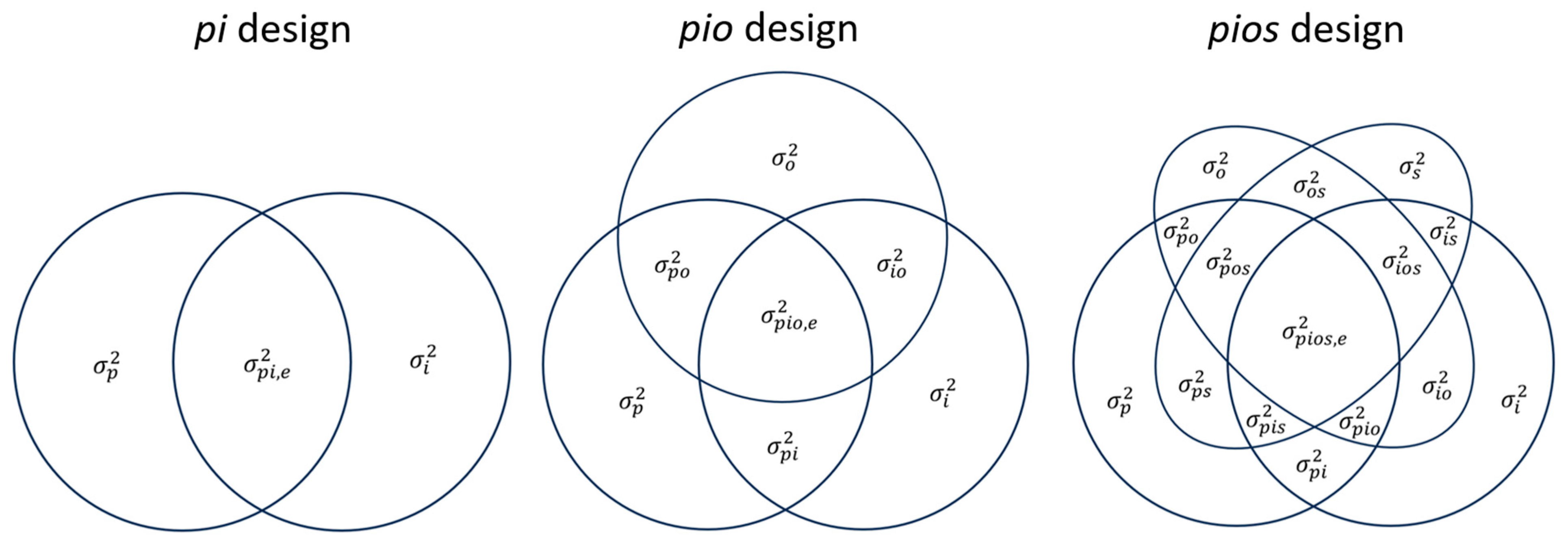
6.2.1. persons × items (pi) designs

In

Table 4. G and global D coefficients and variance components for GT persons × items designs using ULS estimation.

Scale Metric/Index	Procedure
	GENOVA	gtheory Package in R	Jorgensen	Indicator Mean
2-point metric
G coefficient	0.942	0.942	0.942 (0.924, 0.959)	0.942 (0.924, 0.959)
Global D coefficient	0.940	0.940	0.940 (0.921, 0.955)	0.940 (0.921, 0.955)
${\widehat{\sigma }}_p^2$	0.134	0.134	0.134 (0.124, 0.145)	0.134 (0.124, 0.145)
${\widehat{\sigma }}_{pi,e}^2$	0.099	0.099	0.099 (0.072, 0.127)	0.099 (0.072, 0.127)
${\widehat{\sigma }}_i^2$	0.004	0.004	0.004 (0.003, 0.010)	0.004 (0.003, 0.010)
4-point metric
G coefficient	0.959	0.959	0.959 (0.956, 0.962)	0.959 (0.956, 0.962)
Global D coefficient	0.957	0.957	0.957 (0.954, 0.960)	0.957 (0.954, 0.960)
${\widehat{\sigma }}_p^2$	0.765	0.765	0.765 (0.754, 0.775)	0.765 (0.754, 0.775)
${\widehat{\sigma }}_{pi,e}^2$	0.389	0.389	0.389 (0.362, 0.416)	0.389 (0.362, 0.416)
${\widehat{\sigma }}_i^2$	0.023	0.023	0.024 * (0.018, 0.035)	0.024 * (0.018, 0.035)
8-point metric
G coefficient	0.965	0.965	0.965 (0.964, 0.965)	0.965 (0.964, 0.965)
Global D coefficient	0.963	0.963	0.962 * (0.962, 0.963)	0.962 * (0.962, 0.963)
${\widehat{\sigma }}_p^2$	3.355	3.355	3.355 (3.344, 3.366)	3.355 (3.344, 3.366)
${\widehat{\sigma }}_{pi,e}^2$	1.471	1.470 *	1.470 * (1.442, 1.497)	1.470 * (1.442, 1.497)
${\widehat{\sigma }}_i^2$	0.096	0.096	0.099 * (0.085, 0.118)	0.099 * (0.085, 0.118)

Note. GT = generalizability theory, ULS = Unweighted Least Squares estimation, p = persons, i = items, and ,e = remaining relative residual error. Values within parentheses represent 95% Monte Carlo confidence interval limits [56]. All results reported in the tables are based on ${n\prime }_i=12.$ Values that differ with those from GENOVA in the table are marked with asterisks.

, we report variance components, G coefficients, and global D coefficients for observed scores within the pi designs obtained from GENOVA, the gtheory package in R, and the two SEM procedures (Jorgensen’s and our new method). For the two-point scale metric, results are identical across all procedures, with estimated G and global D coefficients, respectively, equaling 0.942 and 0.940, and 95% confidence intervals for all indices within the SEM analyses failing to capture zero. For the four-point metric, results are also identical across procedures except for the variance component for items being 0.001 higher (0.024 vs. 0.023) in the two SEM analyses compared to the two conventional packages. G and global D coefficients for four scale points further increase to 0.959 and 0.957, respectively, and the 95% confidence intervals for all indices again fail to capture zero. For the eight-point metric, results are identical for the SEM procedures and identical for the two conventional procedures except for the pi,e variance component (1.471 vs. 1.470), but these pairs of methods differ slightly from each other, with the global D coefficient for the SEM procedures being 0.001 lower (0.962 vs. 0.963) and the i variance component being 0.003 higher (0.099 vs. 0.096). Across procedures, the G coefficient for the eight-point metric equals 0.965, but the difference between it and the G coefficient for the four-point scale (0.965 − 0.959 = 0.006) is noticeably smaller than the difference in G coefficients between the two- and four-point scales (0.959 − 0.942 = 0.017). This same trend of diminishing improvement in accuracy with increases in numbers of scale points holds for global D coefficients and for each of the conventional reliability coefficients previously reported in Table 3.

One of the key advantages of doing GT analyses using SEMs is that estimation procedures such as WLSMV can be used to adjust for scale coarseness effects resulting from limited numbers of response options and/or unequal intervals between those options by referencing results to a continuous latent response variable metric. Such results for G and global D coefficients, in turn, can serve as estimated upper bounds for score accuracy that might be achieved by increasing number of scale points. WLSMV estimation results reported in

Table 5. G and global D coefficients and variance components for GT persons × items designs using WLSMV estimation.

Scale Point/Index	Procedure
	Jorgensen	Indicator Mean
2-point metric
G coefficient	0.986 (0.982, 0.989)	0.986 (0.982, 0.989)
Global D coefficient	0.983 (0.979, 0.986)	0.983 (0.979, 0.986)
${\widehat{\sigma }}_p^2$	5.899 (4.612, 7.185)	5.899 (4.612, 7.184)
${\widehat{\sigma }}_{pi,e}^2$	1.000 (1.000, 1.000)	1.000 (1.000, 1.000)
${\widehat{\sigma }}_i^2$	0.199 (0.138, 0.290)	0.199 (0.138, 0.290)
4-point metric
G coefficient	0.980 (0.976, 0.982)	0.980 (0.976, 0.982)
Global D coefficient	0.977 (0.973, 0.980)	0.977 (0.973, 0.980)
${\widehat{\sigma }}_p^2$	4.032 (3.388, 4.675)	4.032 (3.388, 4.674)
${\widehat{\sigma }}_{pi,e}^2$	1.000 (1.000, 1.000)	1.000 (1.000, 1.000)
${\widehat{\sigma }}_i^2$	0.123 (0.093, 0.166)	0.123 (0.093, 0.166)
8-point metric
G coefficient	0.979 (0.976, 0.982)	0.979 (0.976, 0.982)
Global D coefficient	0.977 (0.973, 0.980)	0.977 (0.973, 0.980)
${\widehat{\sigma }}_p^2$	3.966 (3.398, 4.534)	3.966 (3.398, 4.534)
${\widehat{\sigma }}_{pi,e}^2$	1.000 (1.000, 1.000)	1.000 (1.000, 1.000)
${\widehat{\sigma }}_i^2$	0.109 (0.083, 0.144)	0.109 (0.083, 0.144)

Note. GT = generalizability theory, WLSMV = Weighted Least Squares Mean and Variance adjusted estimation, p = persons, i = items, and ,e = remaining relative residual error. Values within parentheses represent 95% Monte Carlo confidence interval limits [56]. All results reported in the table are based on ${n\prime }_i=12.$

are identical for the two SEM procedures in relation to variance components, G coefficients, and global D coefficients, and all corresponding 95% confidence intervals again fail to capture zero. In comparison to the observed score results previously described, G and global D coefficients, respectively, increase from 0.942 and 0.940 to 0.986 and 0.983 for the two-point metric; from 0.959 and 0.957 to 0.980 and 0.977 for the four-point metric, and from 0.965 and 0.963 to 0.979 and 0.977 on the eight-point metric. As would be expected, results for G and global D coefficients are more consistent across numbers of response options using WLSMV because, in all instances, they are referenced to a continuous metric rather than varying discrete scale score metrics, with differences in score accuracy between WLSMV and ULS estimates diminishing with increases in number of original raw score scale points.

6.2.2. persons × items × occasions (pio) designs

Congruence in observed score results across the four procedures continues to hold for the pio design, with no differences among variance components, G coefficients, and global D coefficients for the two-point scale; differences no larger than 0.001 for the four-point scales; and differences no greater than 0.002 for the eight-point scale (see

Table 6. G and global D coefficients and variance components for GT persons × items × occasions designs using ULS estimation.

Scale Point/Index	Procedure
	GENOVA	gtheory Package in R	Jorgensen	Indicator Mean
2-point
G coefficient	0.884	0.884	0.884 (0.821, 0.951)	0.884 (0.821, 0.951)
Global D coefficient	0.882	0.882	0.882 (0.816, 0.946)	0.882 (0.817, 0.947)
${\widehat{\sigma }}_p^2$	0.132	0.132	0.132 (0.125, 0.140)	0.132 (0.125, 0.140)
${\widehat{\sigma }}_{pi}^2$	0.016	0.016	0.016 (−0.010, 0.043)	0.016 (−0.010, 0.043)
${\widehat{\sigma }}_{po}^2$	0.010	0.010	0.010 (−0.001, 0.020)	0.010 (−0.001, 0.020)
${\widehat{\sigma }}_{pio,e}^2$	0.077	0.077	0.077 (0.044, 0.109)	0.077 (0.044, 0.109)
${\widehat{\sigma }}_i^2$	0.004	0.004	0.004 (0.003, 0.007)	0.004 (0.003, 0.007)
${\widehat{\sigma }}_o^2$	0.000	0.000	0.000 (0.000, 0.001)	0.000 (0.000, 0.001)
${\widehat{\sigma }}_{io}^2$	0.000	0.000	0.000 (0.001, 0.004)	0.000 (0.000, 0.002)
4-point
G coefficient	0.905	0.905	0.905 (0.893, 0.917)	0.905 (0.893, 0.917)
Global D coefficient	0.902	0.902	0.902 (0.890, 0.914)	0.902 (0.890, 0.914)
${\widehat{\sigma }}_p^2$	0.742	0.742	0.742 (0.734, 0.749)	0.742 (0.734, 0.749)
${\widehat{\sigma }}_{pi}^2$	0.058	0.058	0.058 (0.032, 0.084)	0.058 (0.032, 0.084)
${\widehat{\sigma }}_{po}^2$	0.050	0.050	0.050 (0.039, 0.061)	0.050 (0.039, 0.061)
${\widehat{\sigma }}_{pio,e}^2$	0.281	0.281	0.281 (0.249, 0.314)	0.281 (0.249, 0.314)
${\widehat{\sigma }}_i^2$	0.021	0.021	0.022 * (0.017, 0.028)	0.022 * (0.017, 0.028)
${\widehat{\sigma }}_o^2$	0.000	0.000	0.001 * (0.000, 0.002)	0.001 * (0.000, 0.002)
${\widehat{\sigma }}_{io}^2$	0.000	0.000	0.001 * (0.001, 0.005)	0.000 (0.000, 0.003)
8-point
G coefficient	0.913	0.913	0.913 (0.910, 0.916)	0.913 (0.910, 0.916)
Global D coefficient	0.911	0.911	0.910 * (0.908, 0.913)	0.911 (0.908, 0.913)
${\widehat{\sigma }}_p^2$	3.251	3.251	3.251 (3.243, 3.258)	3.251 (3.243, 3.258)
${\widehat{\sigma }}_{pi}^2$	0.237	0.237	0.237 (0.210, 0.263)	0.237 (0.210, 0.263)
${\widehat{\sigma }}_{po}^2$	0.204	0.204	0.204 (0.193, 0.214)	0.204 (0.193, 0.214)
${\widehat{\sigma }}_{pio,e}^2$	1.037	1.037	1.037 (1.004, 1.070)	1.037 (1.005, 1.070)
${\widehat{\sigma }}_i^2$	0.087	0.087	0.089 * (0.079, 0.102)	0.089 * (0.079, 0.102)
${\widehat{\sigma }}_o^2$	0.001	0.001	0.002 * (0.000, 0.005)	0.002 * (0.000, 0.005)
${\widehat{\sigma }}_{io}^2$	0.002	0.002	0.003 * (0.002, 0.009)	0.002 (0.001, 0.005)

Note. GT = generalizability theory, ULS = Unweighted Least Squares estimation, p = persons, i = items, o = occasions, and ,e = remaining relative residual error. Values within parentheses represent 95% Monte Carlo confidence interval limits [56]. All results reported in the tables are based on ${n\prime }_i=12 \mathrm{a}\mathrm{n}\mathrm{d} {n\prime }_o=1.$ Values that differ with those from GENOVA in the table are marked with asterisks.

). Except for the global D coefficient on the eight-point scale for Jorgensen’s method (0.910), the magnitudes of G and global D coefficients do not vary across the four procedures, respectively, equaling 0.884 and 0.882 for the two-point metric, 0.905 and 0.902 for the four-point metric, and 0.913 and 0.911 for the eight-point metric. Values for these coefficients are lower than corresponding ones from the pi design due to inclusion of another estimated source of measurement error (occasions). The slight differences in indices that appear across procedures are generally between the traditional GT and SEM analyses. In contrast to results for the pi design, several of the 95% confidence intervals within the pio design capture zero, including the pi, po, o, and io variance components for the two-point scale; the o and io variance components for the four-point scale; and the o variance component for the eight-point scale. The preponderance of confidence intervals that capture zero involving occasions makes sense because perceptions of composing skills were not expected to change appreciatively across the first week gap between administrations of the MUSPI.

Results for WLSMV estimates in

Table 7. G and global D coefficients and variance components for GT persons × items × occasions design using WLSMV estimation.

Scale Point/Index	Procedure
	Jorgensen	Indicator Mean
2-point
G coefficient	0.920 (0.896, 0.937)	0.920 (0.896, 0.937)
Global D coefficient	0.917 (0.893, 0.935)	0.917 (0.893, 0.935)
${\widehat{\sigma }}_p^2$	11.570 (8.294, 14.839)	11.570 (8.297, 14.842)
${\widehat{\sigma }}_{pi}^2$	0.717 (0.429, 1.003)	0.717 (0.431, 1.003)
${\widehat{\sigma }}_{po}^2$	0.864 (0.628, 1.101)	0.864 (0.628, 1.101)
${\widehat{\sigma }}_{pio,e}^2$	1.000 (1.000, 1.000)	1.000 (1.000, 1.000)
${\widehat{\sigma }}_i^2$	0.354 (0.241, 0.507)	0.354 (0.242, 0.507)
${\widehat{\sigma }}_o^2$	0.005 (0.000, 0.032)	0.005 (0.000, 0.032)
${\widehat{\sigma }}_{io}^2$	0.013 * (0.010, 0.048)	0.009 (0.007, 0.030)
4-point
G coefficient	0.915 (0.900, 0.927)	0.915 (0.900, 0.927)
Global D coefficient	0.913 (0.896, 0.925)	0.913 (0.897, 0.925)
${\widehat{\sigma }}_p^2$	6.238 (5.170, 7.305)	6.238 (5.171, 7.307)
${\widehat{\sigma }}_{pi}^2$	0.342 (0.281, 0.402)	0.342 (0.281, 0.403)
${\widehat{\sigma }}_{po}^2$	0.466 (0.402, 0.530)	0.466 (0.402, 0.531)
${\widehat{\sigma }}_{pio,e}^2$	1.000 (1.000, 1.000)	1.000 (1.000, 1.000)
${\widehat{\sigma }}_i^2$	0.182 (0.143, 0.233)	0.182 (0.143, 0.233)
${\widehat{\sigma }}_o^2$	0.004 (0.000, 0.017)	0.004 (0.000, 0.017)
${\widehat{\sigma }}_{io}^2$	0.007 * (0.004, 0.019)	0.004 (0.002, 0.010)
8-point
G coefficient	0.899 (0.884, 0.911)	0.899 (0.884, 0.911)
Global D coefficient	0.897 (0.881, 0.909)	0.897 (0.881, 0.909)
${\widehat{\sigma }}_p^2$	6.325 (5.340, 7.308)	6.325 (5.336, 7.310)
${\widehat{\sigma }}_{pi}^2$	0.354 (0.311, 0.397)	0.354 (0.311, 0.397)
${\widehat{\sigma }}_{po}^2$	0.597 (0.543, 0.650)	0.597 (0.543, 0.650)
${\widehat{\sigma }}_{pio,e}^2$	1.000 (1.000, 1.000)	1.000 (1.000, 1.000)
${\widehat{\sigma }}_i^2$	0.167 (0.132, 0.211)	0.167 (0.132, 0.211)
${\widehat{\sigma }}_o^2$	0.004 (0.000, 0.016)	0.004 (0.000, 0.016)
${\widehat{\sigma }}_{io}^2$	0.006 * (0.004, 0.016)	0.003 (0.002, 0.009)

Note. GT = generalizability theory, WLSMV = Weighted Least Squares Mean and Variance adjusted estimation, p = persons, i = items, o = occasions, and ,e = remaining relative residual error. Values within parentheses represent 95% Monte Carlo confidence interval limits [56]. All results reported in the tables are based on ${n\prime }_i=12 \mathrm{a}\mathrm{n}\mathrm{d} {n\prime }_o=1.$ Values that differ with those from Indicator Mean procedure in the table are marked with asterisks.

for the pio design are identical for the two SEM procedures except that the io variance component within our procedure is 0.004 lower on the two-point scale and 0.003 lower on the four- and eight-point scales. As with the pi designs, G and global D coefficients within the WLSMV pio designs are more similar in magnitude across numbers of scale points than are those for the ULS designs. Due to the enhanced precision of the WLSMV estimates, the number of confidence intervals capturing zero is reduced and limited to the o variance component across all scale metrics.

6.2.3. persons × items × occasions × skills (pios) design

Observed score results for the pios design reported in

Table 8. G and global D coefficients and variance components for GT persons × items × occasions × skills designs using ULS estimation.

Scale Point/Index	Procedure
	GENOVA	gtheory Package in R	Jorgensen	Indicator Mean
2-point
G coefficient	0.860	0.860	0.860 (0.839, 0.881)	0.860 (0.839, 0.881)
Global D coefficient	0.852	0.852	0.856 * (0.835, 0.876)	0.852 (0.830, 0.871)
${\widehat{\sigma }}_p^2$	0.111	0.111	0.111 (0.109, 0.113)	0.111 (0.109, 0.113)
${\widehat{\sigma }}_{pi}^2$	0.007	0.007	0.007 (−0.001, 0.014)	0.007 (−0.001, 0.014)
${\widehat{\sigma }}_{po}^2$	0.004	0.004	0.004 (0.001, 0.007)	0.004 (0.001, 0.007)
${\widehat{\sigma }}_{ps}^2$	0.042	0.042	0.042 (0.038, 0.046)	0.042 (0.038, 0.046)
${\widehat{\sigma }}_{pio}^2$	0.006	0.006	0.006 (−0.005, 0.016)	0.006 (−0.005, 0.016)
${\widehat{\sigma }}_{pis}^2$	0.008	0.008	0.007 * (−0.008, 0.023)	0.007 * (−0.008, 0.023)
${\widehat{\sigma }}_{pos}^2$	0.005	0.005	0.005 (−0.001, 0.012)	0.005 (−0.001, 0.012)
${\widehat{\sigma }}_{pios,e}^2$	0.063	0.063	0.063 (0.043, 0.082)	0.063 (0.043, 0.082)
${\widehat{\sigma }}_i^2$	0.002	0.002	0.001 * (0.000, 0.001)	0.002 (0.001, 0.003)
${\widehat{\sigma }}_o^2$	0.000	0.000	0.000 (0.000, 0.000)	0.000 (0.000, 0.001)
${\widehat{\sigma }}_s^2$	0.004	0.004	0.002 * (0.001, 0.002)	0.004 (0.003, 0.005)
${\widehat{\sigma }}_{io}^2$	0.000	0.000	0.000 (0.000, 0.001)	0.000 (0.000, 0.001)
${\widehat{\sigma }}_{is}^2$	0.000	0.000	0.000 (0.001, 0.002)	0.000 (0.001, 0.002)
${\widehat{\sigma }}_{os}^2$	0.000	0.000	0.000 (0.000, 0.001)	0.000 (0.000, 0.000)
${\widehat{\sigma }}_{ios}^2$	0.000	0.000	0.000 (0.000, 0.001)	0.000 (0.000, 0.001)
4-point
G coefficient	0.884	0.884	0.884 (0.881, 0.887)	0.884 (0.880, 0.887)
Global D coefficient	0.876	0.876	0.880 * (0.876, 0.883)	0.876 (0.872, 0.879)
${\widehat{\sigma }}_p^2$	0.717	0.717	0.717 (0.715, 0.719)	0.717 (0.715, 0.719)
${\widehat{\sigma }}_{pi}^2$	0.027	0.027	0.027 (0.019, 0.034)	0.027 (0.020, 0.035)
${\widehat{\sigma }}_{po}^2$	0.025	0.025	0.025 (0.022, 0.028)	0.025 (0.022, 0.028)
${\widehat{\sigma }}_{ps}^2$	0.219	0.219	0.219 (0.214, 0.223)	0.219 (0.214, 0.223)
${\widehat{\sigma }}_{pio}^2$	0.019	0.019	0.019 (0.008, 0.030)	0.019 (0.010, 0.031)
${\widehat{\sigma }}_{pis}^2$	0.026	0.026	0.026 (0.011, 0.041)	0.026 (0.013, 0.043)
${\widehat{\sigma }}_{pos}^2$	0.021	0.021	0.021 (0.015, 0.027)	0.021 (0.015, 0.028)
${\widehat{\sigma }}_{pios,e}^2$	0.237	0.237	0.237 (0.218, 0.257)	0.237 (0.218, 0.257)
${\widehat{\sigma }}_i^2$	0.016	0.016	0.005 * (0.005, 0.006)	0.017 * (0.015, 0.019)
${\widehat{\sigma }}_o^2$	0.001	0.001	0.000 * (0.000, 0.001)	0.001 (0.000, 0.002)
${\widehat{\sigma }}_s^2$	0.020	0.020	0.008 * (0.007, 0.010)	0.021 * (0.018, 0.024)
${\widehat{\sigma }}_{io}^2$	0.000	0.000	0.002 * (0.001, 0.002)	0.000 (0.000, 0.001)
${\widehat{\sigma }}_{is}^2$	0.002	0.002	0.002 (0.002, 0.003)	0.002 (0.002, 0.003)
${\widehat{\sigma }}_{os}^2$	0.000	0.000	0.002 * (0.002, 0.002)	0.000 (0.000, 0.001)
${\widehat{\sigma }}_{ios}^2$	0.000	0.000	0.000 (0.001, 0.001)	0.001 * (0.001, 0.002)
8-point
G coefficient	0.889	0.889	0.889 (0.888, 0.890)	0.889 (0.888, 0.890)
Global D coefficient	0.882	0.882	0.884 * (0.883, 0.885)	0.882 (0.881, 0.883)
${\widehat{\sigma }}_p^2$	3.183	3.183	3.183 (3.181, 3.185)	3.183 (3.181, 3.185)
${\widehat{\sigma }}_{pi}^2$	0.112	0.112	0.112 (0.105, 0.120)	0.112 (0.105, 0.120)
${\widehat{\sigma }}_{po}^2$	0.114	0.114	0.114 (0.110, 0.117)	0.114 (0.110, 0.117)
${\widehat{\sigma }}_{ps}^2$	0.908	0.908	0.908 (0.904, 0.912)	0.908 (0.904, 0.912)
${\widehat{\sigma }}_{pio}^2$	0.075	0.075	0.075 (0.064, 0.085)	0.075 (0.064, 0.085)
${\widehat{\sigma }}_{pis}^2$	0.099	0.099	0.099 (0.084, 0.114)	0.099 (0.084, 0.114)
${\widehat{\sigma }}_{pos}^2$	0.083	0.083	0.083 (0.077, 0.089)	0.083 (0.077, 0.089)
${\widehat{\sigma }}_{pios,e}^2$	0.858	0.858	0.858 (0.839, 0.877)	0.858 (0.839, 0.877)
${\widehat{\sigma }}_i^2$	0.065	0.065	0.022 * (0.021, 0.024)	0.068 * (0.064, 0.073)
${\widehat{\sigma }}_o^2$	0.002	0.002	0.003 * (0.002, 0.004)	0.003 * (0.002, 0.004)
${\widehat{\sigma }}_s^2$	0.081	0.081	0.066 * (0.063, 0.070)	0.083 * (0.078, 0.090)
${\widehat{\sigma }}_{io}^2$	0.001	0.001	0.006 * (0.006, 0.007)	0.001 (0.001, 0.002)
${\widehat{\sigma }}_{is}^2$	0.008	0.008	0.008 (0.008, 0.011)	0.007 * (0.006, 0.009)
${\widehat{\sigma }}_{os}^2$	0.000	0.000	0.001 * (0.001, 0.001)	0.000 (0.000, 0.001)
${\widehat{\sigma }}_{ios}^2$	0.001	0.001	0.001 (0.001, 0.002)	0.001 (0.001, 0.002)

Note. GT = generalizability theory, ULS = Unweighted Least Squares estimation, p = persons, i = items, o = occasions, s = skills, and ,e = remaining relative residual error. Values within parentheses represent 95% Monte Carlo confidence interval limits [56]. All results reported in the tables are based on ${n\prime }_i=12, {n\prime }_o=1, \mathrm{a}\mathrm{n}\mathrm{d} {n\prime }_s=4.$ Values that differ with those from GENOVA in the table are marked with asterisks.

on the two-point metric vary by no more than 0.004 across the conventional and SEM procedures, but those for Jorgensen’s SEM method begin to diverge more from those for the other procedures on the four- and eight-point scales. Indices for the two conventional procedures and our SEM procedure vary by no more than 0.001 on the four-point matric and 0.003 on the eight-point metric, whereas differences between Jorgensen’s SEM and the other procedures vary by as much as 0.012 for the s variance component on the four-point metric and by 0.043 for the i variance component on the eight-point metric. Confidence intervals based on our procedure capture zero for the pi, pio, pis, pos, o, io, os, and ios variance components on the two-point metric, for the o, io, and os variance components on the four-point metric, and for the os variance component on the eight-point metric. As in the previous two designs, differences between G and global D coefficients are greater between the two- and four-point metrics than between the four- and eight-point metrics.

Within the WLSMV analyses reported in

Table 9. G and global D coefficients and variance components for GT persons × items × occasions × skills designs using WLSMV estimation.

Scale Point/ Index	Procedure
	Jorgensen	Indicator Mean
2-point
G coefficient	0.899 (0.877, 0.918)	0.899 (0.877, 0.918)
Global D coefficient	0.895 * (0.872, 0.913)	0.890 (0.866, 0.909)
${\widehat{\sigma }}_p^2$	23.544 * (15.012, 32.092)	23.541 (15.002, 32.083)
${\widehat{\sigma }}_{pi}^2$	1.098 (0.591, 1.613)	1.098 (0.588, 1.610)
${\widehat{\sigma }}_{po}^2$	0.843 * (0.482, 1.208)	0.844 (0.481, 1.207)
${\widehat{\sigma }}_{ps}^2$	5.875 (3.698, 8.057)	5.875 (3.713, 8.050)
${\widehat{\sigma }}_{pio}^2$	0.797 (0.294, 1.302)	0.797 (0.296, 1.298)
${\widehat{\sigma }}_{pis}^2$	0.200 * (−0.057, 0.456)	0.199 (−0.057, 0.457)
${\widehat{\sigma }}_{pos}^2$	0.564 (0.308, 0.820)	0.564 (0.308, 0.819)
${\widehat{\sigma }}_{pios,e}^2$	1.000 (1.000, 1.000)	1.000 (1.000, 1.000)
${\widehat{\sigma }}_i^2$	0.142 * (0.088, 0.214)	0.435 (0.270, 0.655)
${\widehat{\sigma }}_o^2$	0.016 * (0.002, 0.045)	0.029 (0.003, 0.080)
${\widehat{\sigma }}_s^2$	0.340 * (0.198, 0.535)	0.852 (0.497, 1.339)
${\widehat{\sigma }}_{io}^2$	0.044 * (0.032, 0.070)	0.010 (0.006, 0.025)
${\widehat{\sigma }}_{is}^2$	0.090 * (0.066, 0.146)	0.079 (0.058, 0.133)
${\widehat{\sigma }}_{os}^2$	0.076 * (0.046, 0.120)	0.002 (0.000, 0.012)
${\widehat{\sigma }}_{ios}^2$	0.011 * (0.012, 0.031)	0.012 (0.013, 0.032)
4-point
G coefficient	0.900 (0.883, 0.914)	0.900 (0.883, 0.914)
Global D coefficient	0.895 * (0.877, 0.909)	0.892 (0.873, 0.907)
${\widehat{\sigma }}_p^2$	8.783 (7.232, 10.336)	8.783 (7.236, 10.333)
${\widehat{\sigma }}_{pi}^2$	0.312 (0.237, 0.387)	0.312 (0.237, 0.387)
${\widehat{\sigma }}_{po}^2$	0.370 (0.288, 0.453)	0.370 (0.288, 0.453)
${\widehat{\sigma }}_{ps}^2$	2.059 (1.765, 2.355)	2.059 (1.765, 2.355)
${\widehat{\sigma }}_{pio}^2$	0.160 (0.103, 0.218)	0.160 (0.104, 0.217)
${\widehat{\sigma }}_{pis}^2$	0.091 (0.046, 0.136)	0.091 (0.046, 0.136)
${\widehat{\sigma }}_{pos}^2$	0.118 (0.080, 0.156)	0.118 (0.080, 0.156)
${\widehat{\sigma }}_{pios,e}^2$	1.000 (1.000, 1.000)	1.000 (1.000, 1.000)
${\widehat{\sigma }}_i^2$	0.068 * (0.061, 0.078)	0.199 (0.156, 0.252)
${\widehat{\sigma }}_o^2$	0.001 * (0.000, 0.006)	0.008 (0.001, 0.022)
${\widehat{\sigma }}_s^2$	0.113 * (0.084, 0.151)	0.255 (0.178, 0.356)
${\widehat{\sigma }}_{io}^2$	0.083 * (0.076, 0.092)	0.003 (0.002, 0.006)
${\widehat{\sigma }}_{is}^2$	0.028 * (0.024, 0.038)	0.019 (0.015, 0.028)
${\widehat{\sigma }}_{os}^2$	0.045 * (0.035, 0.057)	0.001 (0.000, 0.003)
${\widehat{\sigma }}_{ios}^2$	0.002 * (0.003, 0.007)	0.003 (0.003, 0.007)
8-point
G coefficient	0.891 (0.875, 0.904)	0.891 (0.875, 0.904)
Global D coefficient	0.773 * (0.743, 0.796)	0.884 (0.867, 0.898)
${\widehat{\sigma }}_p^2$	10.150 * (8.463, 11.839)	10.149 (8.462, 11.840)
${\widehat{\sigma }}_{pi}^2$	0.354 (0.286, 0.422)	0.354 (0.286, 0.422)
${\widehat{\sigma }}_{po}^2$	0.460 (0.373, 0.547)	0.460 (0.374, 0.546)
${\widehat{\sigma }}_{ps}^2$	2.424 (2.139, 2.710)	2.424 (2.140, 2.709)
${\widehat{\sigma }}_{pio}^2$	0.193 (0.140, 0.245)	0.193 (0.140, 0.245)
${\widehat{\sigma }}_{pis}^2$	0.194 (0.150, 0.237)	0.194 (0.150, 0.237)
${\widehat{\sigma }}_{pos}^2$	0.407 * (0.368, 0.445)	0.406 (0.368, 0.445)
${\widehat{\sigma }}_{pios,e}^2$	1.000 (1.000, 1.000)	1.000 (1.000, 1.000)
${\widehat{\sigma }}_i^2$	0.212 * (0.201, 0.225)	0.207 (0.162, 0.260)
${\widehat{\sigma }}_o^2$	1.254 * (1.154, 1.360)	0.008 (0.001, 0.023)
${\widehat{\sigma }}_s^2$	0.888 * (0.776, 1.010)	0.258 (0.181, 0.361)
${\widehat{\sigma }}_{io}^2$	0.364 * (0.351, 0.378)	0.003 (0.002, 0.006)
${\widehat{\sigma }}_{is}^2$	0.261 * (0.256, 0.271)	0.022 (0.018, 0.031)
${\widehat{\sigma }}_{os}^2$	0.861 * (0.828, 0.898)	0.001 (0.000, 0.003)
${\widehat{\sigma }}_{ios}^2$	0.003 (0.003, 0.007)	0.003 (0.003, 0.007)

Note. GT = generalizability theory, WLSMV = Weighted Least Squares Mean and Variance adjusted estimation, p = persons, i = items, o = occasions, s = skills, and ,e = remaining relative residual error. Values within parentheses represent 95% Monte Carlo confidence interval limits [56]. All results reported in the tables are based on ${n\prime }_i=12, {n\prime }_o=1, \mathrm{a}\mathrm{n}\mathrm{d} {n\prime }_s=4.$ Values that differ with the Indicator Mean procedure in the table are marked with asterisks.

, discrepancies in indices between the Indicator Mean and Jorgensen’s procedures are even more pronounced, with differences observed for all but one variance component reflecting absolute differences in scores (i.e., the ios variance component for the original eight-point metric). The largest such difference equals 1.246 for the o variance component in relation to the original eight-point metric, with differences in variance components for absolute differences in scores together leading to a counterintuitive global D coefficient of 0.773 for Jorgensen’s procedure versus 0.884 for our procedure when the G coefficient equals 0.891 for both SEM procedures. Overall, these results cast doubt on the appropriateness of using Jorgensen’s procedure for estimating absolute error indices within three-facet GT designs, and especially when scales have eight response options.

6.3. Cut-Score-Specific D Coefficients

In Figure 2, we provide indicator mean method-based cut-score-specific D coefficients in six panels to represent each design and estimation procedure, with the two-, four-, and eight-point scale results represented by Z scores (i.e., standard deviation distances away from the scale mean) for comparative purposes. Conceptually, cut-score-specific D coefficients reflect proportions of random agreement in classifying scores above or below targeted cut points along the assessment continuum when making criterion-referenced decisions [65,66,67]. Consistent with the results for global D coefficients already discussed, differences in cut-score-specific D coefficients are more congruent across numbers of scale points on continuous latent response variable than on observed score metrics, with differences between the coefficients for ULS and WLSMV estimation diminishing with increases in the number of original scale points. As is typically the case, within each panel, the magnitude of D coefficients increases as cut scores get further and further away from the mean of each scale.

7. Discussion

7.1. Overview

Applications of GT analyses within SEM frameworks has steadily increased over recent years. At first, these analyses were limited to estimation of variance components reflecting relative differences in scores (see, e.g., [38,39,40,41,42,43]), but Jorgensen [44] recently extended those frameworks to allow for derivation of variance components reflecting absolute differences in scores within one- and two-facet designs. Subsequently, applications of Jorgensen’s procedures to data collected in live assessment settings using these same designs confirmed that they yielded results highly comparable to those obtained from standalone GT packages and variance components estimation programs within popular comprehensive statistical packages such as SPSS, SAS, and R [14,46,68]. Our goal in the study reported here was to offer an alternative approach to deriving variance components reflecting absolute differences in scores that we believed to be more versatile and widely applicable than Jorgensen’s procedure. To investigate the effectiveness of our new indicator mean-based method, we compared results from it to those obtained using Jorgensen’s SEM procedure and the GT packages GENOVA [57] and gtheory in R [58,59].

7.2. Discrepancies between SEM Methods for Estimating Absolute Error Indices

In keeping with previous research [14,44,46,68], Jorgensen’s procedure yielded results highly comparable to those obtained from the GENOVA package and gtheory package in R for one- and two-facet random effects GT designs, but this proved to be less so overall for three-facet designs, and particularly for those in which items had eight scale points. In contrast, congruence of results between our indicator mean-based procedure and those from the conventional GT packages continued to hold for three-facet designs for any number of scale points considered here. The consistency between our method results and those from the conventional packages occurs because facet condition means derived from our procedure uses indicator intercepts that directly match observed score means obtained from standard ANOVA-based techniques. Moreover, implementing our procedure for deriving absolute errors does not introduce any additional parameters to estimate. As a result, our method remains unaffected by the complexity of the model or the number of scale points, ensuring robust and accurate variance component estimation across various designs. The precision achieved by our procedure, in turn, generalizes well to estimation procedures such as WLSMV when observed score results are transformed to continuous latent response variable metrics.

The discrepancies in absolute error variance components and D coefficients between our procedure and Jorgensen’s are likely due to the extra steps needed to get factor means and indicator intercepts to align with effect coding constraints as facet conditions and numbers of scale points increase. As facet conditions and scale points increase, additional parameter estimates and iterations are needed for optimal fitting. For example, when analyzing the pios design with eight scale points and ULS estimation, our procedure entailed 49 iterations, 291 model parameters, and 187 equality constraints, whereas Jorgensen’s procedure required 66 iterations, 390 model parameters, and 292 equality constraints. As model complexity increases, deviations from effect coding constraints that force the sum of indicator intercepts for each factor to equal zero increase with more scale points, potentially leading to less accurate variance component estimates.

7.3. Summary of Advantages of the Indicator Mean-Based Method and Future Applications

The primary advantages of our indicator mean-based procedure over Jorgensen’s procedure in deriving indices related to absolute error demonstrated here include: (1) use of fewer constraints within SEMs to derive absolute error indices, (2) inclusion of indicator intercepts within SEMs that directly match observed score means, (3) formulas for estimating absolute error variance components that more directly match those within ANOVA-based analyses, (4) more precise estimation of absolute error variance components for designs that include more than two facets and multiple scale points, and (5) extensions to estimation procedures within such analyses that more accurately correct for scale coarseness effects. At a more general level, the present results also highlighted improvements in score accuracy gained when increasing numbers of observed scale points using ULS estimates and the importance of taking all relevant sources of measurement error into account when estimating score generalizability and dependability across all designs. Our extended online Supplementary Material includes code in R for implementing all procedures we illustrated here within one-, two-, and three-facet random effects GT designs. The same techniques are directly applicable to any set of facets including raters for subjectively scored measures.

Although not demonstrated explicitly here, our procedure also can be extended to multivariate and bifactor GT designs with any number of facet conditions and scale points and to derive variance components for absolute error and D coefficients for GT-based designs that allow for congeneric relationships between indicators and underlying factors. We currently are completing research studies to investigate these applications and to extend hypothesis testing procedures for comparing the magnitudes of single-occasion alpha and omega coefficients developed by Deng and Chan [72] to comparisons of G coefficients derived from multi-facet GT designs representing essential tau-equivalent versus congeneric relationships. Collectively, we believe that such applications will go a long way in combining and broadening the benefits of GT and contemporary SEM techniques.

References

1. Cronbach, L.J.; Rajaratnam, N.; Gleser, G.C. Theory of generalizability: A liberalization of reliability theory. Br. J. Stat. Psychol. 1963, 16, 137–163. [Google Scholar] [CrossRef]
2. Cronbach, L.J.; Gleser, G.C.; Nanda, H.; Rajaratnam, N. The Dependability of Behavioral Measurements: Theory of Generalizability for Scores and Profiles; Wiley: New York, NY, USA, 1972. [Google Scholar]
3. Shavelson, R.J.; Webb, N.M. Generalizability Theory: A Primer; Sage: Thousand Oaks, CA, USA, 1991. [Google Scholar]
4. Brennan, R.L. Generalizability Theory; Springer: New York, NY, USA, 2001. [Google Scholar]
5. Chen, D.; Hebert, M.; Wilson, J. Examining human and automated ratings of elementary students’ writing quality: A multivariate generalizability theory application. Am. Educ. Res. J. 2022, 59, 1122–1156. [Google Scholar] [CrossRef]
6. Anderson, T.N.; Lau, J.N.; Shi, R.; Sapp, R.W.; Aalami, L.R.; Lee, E.W.; Tekian, A.; Park, Y.S. The utility of peers and trained raters in technical skill-based assessments a generalizability theory study. J. Surg. Educ. 2022, 79, 206–215. [Google Scholar] [CrossRef]
7. Tindal, G.; Yovanoff, P.; Geller, J.P. Generalizability theory applied to reading assessments for students with significant cognitive disabilities. J. Spec. Educ. 2010, 44, 3–17. [Google Scholar] [CrossRef]
8. Mantzicopoulos, P.; French, B.F.; Patrick, H.; Watson, J.S.; Ahn, I. The stability of kindergarten teachers’ effectiveness: A generalizability study comparing the framework for teaching and the classroom assessment scoring system. Educ. Assess. 2018, 23, 24–46. [Google Scholar] [CrossRef]
9. Lightburn, S.; Medvedev, O.N.; Henning, M.A.; Chen, Y. Investigating how students approach learning using generalizability theory. High. Educ. Res. Dev. 2021, 41, 1618–1632. [Google Scholar] [CrossRef]
10. Ohta, R.; Plakans, L.M.; Gebril, A. Integrated writing scores based on holistic and multi-trait scales: A generalizability analysis. Assess. Writ. 2018, 38, 21–36. [Google Scholar] [CrossRef]
11. Shin, J. Investigating and optimizing score dependability of a local ITA speaking test across language groups: A generalizability theory approach. Lang. Test. 2022, 39, 313–337. [Google Scholar] [CrossRef]
12. Hollo, A.; Staubitz, J.L.; Chow, J.C. Applying generalizability theory to optimize analysis of spontaneous teacher talk in elementary classrooms. J. Speech Lang. Hear. R. 2020, 63, 1947–1957. [Google Scholar] [CrossRef] [PubMed]
13. Bergee, M.J. Performer, rater, occasion, and sequence as sources of variability in music performance assessment. J. Res. Music Educ. 2007, 55, 344–358. [Google Scholar] [CrossRef]
14. Vispoel, W.P.; Lee, H.; Chen, T.; Hong, H. Using structural equation modeling to reproduce and extend ANOVA-based generalizability theory analyses for psychological assessments. Psych 2023, 5, 249–273. [Google Scholar] [CrossRef]
15. Kumar, S.S.; Merkin, A.G.; Numbers, K.; Sachdev, P.S.; Brodaty, H.; Kochan, N.A.; Trollor, J.N.; Mahon, S.; Medvedev, O. A novel approach to investigate depression symptoms in the aging population using generalizability theory. Psychol. Assess 2022, 34, 684–696. [Google Scholar] [CrossRef]
16. Winterstein, B.P.; Willse, J.T.; Kwapil, T.R.; Silvia, P.J. Assessment of score dependability of the Wisconsin Schizotypy Scales using generalizability analysis. J. Psychopathol. Behav. Assess. 2010, 32, 575–585. [Google Scholar] [CrossRef]
17. Truong, Q.C.; Krägeloh, C.U.; Siegert, R.J.; Landon, J.; Medvedev, O.N. Applying generalizability theory to differentiate between trait and state in the Five Facet Mindfulness Questionnaire (FFMQ). Mindfulness 2020, 11, 953–963. [Google Scholar] [CrossRef]
18. LoPilato, A.C.; Carter, N.T.; Wang, M. Updating generalizability theory in management research: Bayesian estimation of variance components. J. Manag. 2015, 41, 692–717. [Google Scholar] [CrossRef]
19. Wang, L.; Finn, A. Measuring CBBE across brand portfolios: Generalizability theory perspective. J. Target. Meas. Anal. Mark. 2012, 20, 109–116. [Google Scholar] [CrossRef]
20. Finn, A. Generalizability modeling of the foundations of customer delight. J. Model. Manag. 2006, 1, 18–32. [Google Scholar] [CrossRef]
21. Highhouse, S.; Broadfoot, A.; Yugo, J.E.; Devendorf, S.A. Examining corporate reputation judgments with generalizability theory. J. Appl. Psychol. 2009, 94, 782. [Google Scholar] [CrossRef]
22. Andersen, S.A.W.; Nayahangan, L.J.; Park, Y.S.; Konge, L. Use of generalizability theory for exploring reliability of and sources of variance in assessment of technical skills: A systematic review and meta-analysis. Acad. Med. 2021, 96, 1609–1619. [Google Scholar] [CrossRef]
23. Lagha, R.A.R.; Boscardin, C.K.; May, W.; Fung, C.C. A comparison of two standard-setting approaches in high-stakes clinical performance assessment using generalizability theory. Acad. Med. 2012, 87, 1077–1082. [Google Scholar] [CrossRef] [PubMed]
24. Spring, A.M.; Pittman, D.J.; Aghakhani, Y.; Jirsch, J.; Pillay, N.; Bello-Espinosa, L.E.; Josephson, C.; Federico, P. Generalizability of high frequency oscillation evaluations in the ripple band. Front. Neurol. 2018, 9, 510. [Google Scholar] [CrossRef]
25. Kreiter, C.; Zaidi, N.B. Generalizability theory’s role in validity research: Innovative applications in health science education. Health Prof. Educ. 2020, 6, 282–290. [Google Scholar] [CrossRef]
26. Kreiter, C.D.; Wilson, A.B.; Humbert, A.J.; Wade, P.A. Examining rater and occasion influences in observational assessments obtained from within the clinical environment. Med. Educ. Online 2016, 21, 29279. [Google Scholar] [CrossRef] [PubMed]
27. Medvedev, O.; Truong, Q.C.; Merkin, A.; Borotkanics, R.; Krishnamurthi, R.; Feigin, V. Cross-cultural validation of the stroke riskometer using generalizability theory. Sci. Rep. 2021, 11, 19064. [Google Scholar] [CrossRef]
28. Preuss, R.A. Using generalizability theory to develop clinical assessment protocols. Phys. Ther. 2013, 93, 562–569. [Google Scholar] [CrossRef]
29. O’Brien, J.; Thompson, M.S.; Hagler, D. Using generalizability theory to inform optimal design for a nursing performance assessment. Eval. Health Prof. 2019, 42, 297–327. [Google Scholar] [CrossRef] [PubMed]
30. Baldwin, S.A.; Larson, M.J.; Clayson, P.E. The dependability of electrophysiological measurements of performance monitoring in a clinical sample: A generalizability and decision analysis of the ERN and Pe. Psychophysiology 2015, 52, 790–800. [Google Scholar] [CrossRef] [PubMed]
31. Carbine, K.A.; Clayson, P.E.; Baldwin, S.A.; LeCheminant, J.; Larson, M.J. Using generalizability theory and the ERP reliability analysis (ERA) toolbox for assessing test- retest reliability of ERP scores Part 2: Application to food- based tasks and stimuli. Int. J. Psychophysiol. 2021, 166, 188–198. [Google Scholar] [CrossRef]
32. Clayson, P.E.; Carbine, K.A.; Baldwin, S.A.; Olsen, J.A.; Larson, M.J. Using generalizability theory and the ERP reliability analysis (ERA) toolbox for assessing test- retest reliability of ERP scores Part 1: Algorithms, framework, and implementation. Int. J. Psychophysiol. 2021, 166, 174–187. [Google Scholar] [CrossRef]
33. Lafave, M.R.; Butterwick, D.J. A generalizability theory study of athletic taping using the Technical Skill Assessment Instrument. J. Athl. Training 2014, 49, 368–372. [Google Scholar] [CrossRef]
34. Wickel, E.E.; Welk, G.J. Applying generalizability theory to estimate habitual activity levels. Med. Sci. Sports Exerc. 2010, 42, 1528–1534. [Google Scholar] [CrossRef] [PubMed]
35. Coussens, A.H.; Rees, T.; Freeman, P. Applying generalizability theory to examine the antecedents of perceived coach support. J. Sport Exerc. Psychol. 2015, 37, 51–62. [Google Scholar] [CrossRef]
36. Jiang, Z.; Raymond, M.; Shi, D.; DiStefano, C. Using a linear mixed-effect model framework to estimate multivariate generalizability theory parameters in R. Behav. Res. Methods 2020, 52, 2383–2393. [Google Scholar] [CrossRef]
37. Vispoel, W.P.; Lee, H.; Hong, H. Applying multivariate generalizability theory to psychological assessments. Psychol. Methods 2023, 1–23. [Google Scholar] [CrossRef] [PubMed]
38. Ark, T.K. Ordinal Generalizability Theory Using an Underlying Latent Variable Framework. Ph.D. Thesis, University of British Columbia, Vancouver, BC, Canada, 2015. Available online: https://open.library.ubc.ca/soa/cIRcle/collections/ubctheses/24/items/1.0166304 (accessed on 23 December 2023).
39. Marcoulides, G.A. Estimating variance components in generalizability theory: The covariance structure analysis approach. Struct. Equ. Modeling 1996, 3, 290–299. [Google Scholar] [CrossRef]
40. Morris, C.A. Optimal Methods for Disattenuating Correlation Coefficients under Realistic Measurement Conditions with Single-Form, Self-Report Instruments (Publication No. 27668419). Ph.D. Thesis, University of Iowa, Iowa City, IA, USA; p. 2020.
41. Raykov, T.; Marcoulides, G.A. Estimation of generalizability coefficients via a structural equation modeling approach to scale reliability evaluation. Int. J. Test. 2006, 6, 81–95. [Google Scholar] [CrossRef]
42. Vispoel, W.P.; Morris, C.A.; Kilinc, M. Applications of generalizability theory and their relations to classical test theory and structural equation modeling. Psychol. Methods 2018, 23, 1–26. [Google Scholar] [CrossRef]
43. Vispoel, W.P.; Morris, C.A.; Kilinc, M. Practical applications of generalizability theory for designing, evaluating, and improving psychological assessments. J. Pers. Assess. 2018, 100, 53–67. [Google Scholar] [CrossRef]
44. Jorgensen, T.D. How to estimate absolute-error components in structural equation models of generalizability theory. Psych 2021, 3, 113–133. [Google Scholar] [CrossRef]
45. Vispoel, W.P.; Morris, C.A.; Kilinc, M. Using generalizability theory with continuous latent response variables. Psychol. Methods 2019, 24, 153–178. [Google Scholar] [CrossRef]
46. Vispoel, W.P.; Hong, H.; Lee, H. Benefits of doing generalizability theory analyses within structural equation modeling frameworks: Illustrations using the Rosenberg Self-Esteem Scale [Teacher’s corner]. Struct. Equ. Model. 2024, 31, 165–181. [Google Scholar] [CrossRef]
47. Vispoel, W.P.; Lee, H.; Chen, T. Estimating Reliability, Measurement Error from Multiple Sources, and Subscale Added Value within Multivariate Structural Equation Model Designs. 2024; manuscript submitted for publication. [Google Scholar]
48. Vispoel, W.P.; Xu, G.; Kilinc, M. Expanding G-theory models to incorporate congeneric relationships: Illustrations using the Big Five Inventory. J. Personal. Assess. 2021, 104, 429–442. [Google Scholar] [CrossRef] [PubMed]
49. Vispoel, W.P.; Xu, G.; Schneider, W.S. Interrelationships between latent state-trait theory and generalizability theory within a structural equation modeling framework. Psychol. Methods 2022, 27, 773–803. [Google Scholar] [CrossRef] [PubMed]
50. Vispoel, W.P.; Lee, H.; Chen, T.; Hong, H. Analyzing and comparing univariate, multivariate, and bifactor generalizability theory designs for hierarchically structured personality traits. J. Pers. Assess. 2023, 1–16. [Google Scholar] [CrossRef] [PubMed]
51. Vispoel, W.P.; Lee, H.; Hong, H. Analyzing multivariate generalizability theory designs within structural equation modeling frameworks. Struct. Equ. Modeling 2023, 1–22. [Google Scholar] [CrossRef]
52. Vispoel, W.P.; Lee, H.; Chen, T.; Hong, H. Extending applications of generalizability theory-based bifactor model designs. Psych 2023, 5, 545–575. [Google Scholar] [CrossRef]
53. Vispoel, W.P.; Lee, H.; Xu, G.; Hong, H. Expanding bifactor models of psychological traits to account for multiple sources of measurement error. Psychol. Assess. 2022, 34, 1093–1111. [Google Scholar] [CrossRef]
54. Vispoel, W.P.; Lee, H.; Xu, G.; Hong, H. Integrating bifactor models into a generalizability theory-based structural equation modeling framework. J. Exp. Educ. 2023, 91, 718–738. [Google Scholar] [CrossRef]
55. Jorgensen, T.D.; Pornprasertmanit, S.; Schoemann, A.M.; Rosseel, Y.; Miller, P.; Quick, C.; Garnier-Villarreal, M.; Selig, J.; Boulton, A.; Preacher, K. Package ‘Semtools’. 2022. Available online: https://cran.r-project.org/web/packages/semTools/semTools.pdf (accessed on 23 December 2023).
56. Preacher, K.J.; Selig, J.P. Advantages of Monte Carlo confidence intervals for indirect effects. Commun. Methods Meas. 2012, 6, 77–98. [Google Scholar] [CrossRef]
57. Crick, J.E.; Brennan, R.L. Manual for GENOVA: A Generalized Analysis of Variance System; American College Testing Technical Bulletin 43; ACT, Inc.: Iowa City, IA, USA, 1983. [Google Scholar]
58. Moore, C.T. gtheory: Apply Generalizability Theory with R. R Package Version 1.2. 2016. Available online: https://CRAN.R-project.org/package=gtheory (accessed on 23 December 2023).
59. Huebner, A.; Lucht, M. Generalizability Theory in R. Pract. Assess. Res. Eval. 2019, 24, 1–12. [Google Scholar]
60. Rosseel, Y. lavaan: An R package for structural equation modeling. J. Stat. Softw. 2012, 48, 1–36. [Google Scholar] [CrossRef]
61. Rosseel, Y.; Jorgensen, T.D.; Rockwood, N. Package ‘lavaan’. R Package Version (0.6-15). 2023. Available online: https://cran.r-project.org/web/packages/lavaan/lavaan.pdf (accessed on 23 December 2023).
62. Vispoel, W.P. Measuring and understanding self-perceptions of musical ability. In International Advances in Self Research; Marsh, H.W., Craven, R.G., McInerney, D.M., Eds.; Information Age: Greenwich, CT, USA, 2003; Volume 1, pp. 151–180. [Google Scholar]
63. Vispoel, W.P. Integrating self-perceptions of music skill into contemporary models of self-concept. Vis. Res. Music. Educ. 2021, 16, 33. [Google Scholar]
64. Vispoel, W.P.; Lee, H. Understanding the Structure of Music Self-Concept from Multiple Analytic Perspectives. In Proceedings of the Annual Meeting of the American Psychological Association, Washington, DC, USA., 5 August 2023. [Google Scholar]
65. Brennan, R.L.; Kane, M.T. An index of dependability for mastery tests. J. Educ. Meas. 1977, 14, 277–289. [Google Scholar] [CrossRef]
66. Kane, M.T.; Brennan, R.L. Agreement coefficients as indices of dependability for domain-referenced tests. Appl. Psych. Meas. 1980, 4, 105–126. [Google Scholar] [CrossRef]
67. Brennan, R.L. Examining the dependability of scores. In R. A. Berk A Guide to Criterion-Referenced Test Construction; John Hopkins University Press: Baltimore, MD, USA, 1984; pp. 293–332. [Google Scholar]
68. Vispoel, W.P.; Hong, H.; Lee, H.; Jorgensen, T.R. Analyzing complete generalizability theory designs using structural equation models. Appl. Meas. Educ. 2023, 36, 372–393. [Google Scholar] [CrossRef]
69. Little, T.D.; Siegers, D.W.; Card, N.A. A non-arbitrary method or identifying and scaling latent variables in SEM and MACS models. Struct. Equ. Model. 2006, 13, 59–72. [Google Scholar] [CrossRef]
70. Bates, D.; Maechler, M.; Bolker, B. Package ‘lme4’. R Package Version (1.1-32). 2023. Available online: https://cran.r-project.org/web/packages/lme4/lme4.pdf (accessed on 23 December 2023).
71. Marcoulides, G.A. An alternative method for estimating variance components in generalizability theory. Psychol. Rep. 1990, 66, 379–386. [Google Scholar] [CrossRef]
72. Deng, L.; Chan, W. Testing the difference between reliability coefficients alpha and omega. Educ. Psychol. Meas. 2017, 77, 185–203. [Google Scholar] [CrossRef]
Figure 1. Diagrams representing complete partitioning of observed score variance within GT pi, pio, and pios designs. Note. GT = generalizability theory, p = persons, i = items, o = occasions, s = skills, and ,e = remaining relative residual error.
Psych 06 00024 g001
Figure 2. Cut-score-specific D coefficients for ULS and WLSMV pi, pio and pios GT designs on Z score (M = 0, SD = 1) metrics. Note. ULS = Unweighted Least Squares estimation, WLSMV = Weighted Least Squares Mean and Variance adjusted estimation, p = persons, i = items, o = occasions, s = skills, and GT = generalizability theory, D coefficient = dependability coefficient.
Psych 06 00024 g002