
Evaluating the Effect of Planned Missing Designs in Structural Equation Model Fit Measures

ECEO, COPELABS, Lusofona University, 1749-024 Lisbon, Portugal
Psych 2023, 5(3), 983-995; https://doi.org/10.3390/psych5030064
Submission received: 7 August 2023
/
Revised: 31 August 2023
/
Accepted: 1 September 2023
/
Published: 6 September 2023
(This article belongs to the Special Issue Feature Papers in Psychometrics and Educational Measurement)
Abstract
:In a planned missing design, the nonresponses occur according to the researcher’s will, with the goal of increasing data quality and avoiding overly extensive questionnaires. When adjusting a structural equation model to the data, there are different criteria to evaluate how the theoretical model fits the observed data, with the root mean square error of approximation (RMSEA), standardized root mean square residual (SRMR), comparative fit index (CFI) and Tucker–Lewis index (TLI) being the most common. Here, I explore the effect of the nonresponses due to a specific planned missing design—the three-form design—on the mentioned fit indices when adjusting a structural equation model. A simulation study was conducted with correctly specified model and one model with misspecified correlation between factors. The CFI, TLI and SRMR indices are affected by the nonresponses, particularly with small samples, low factor loadings and numerous observed variables. The existence of nonresponses when considering misspecified models causes unacceptable values for all the four fit indexes under analysis, namely when a strong correlation between factors is considered. The results shown here were performed with the simsem package in R and the full information maximum-likelihood method was used for handling missing data during model fitting.
1. Introduction
It is usually challenging for researchers to know the exact number of questions that will be answered in a survey, which can lead to incomplete data. Such a challenge can be overcome by either imposing a limit to the number of questions in the survey or using a planned missing design. The latter allows the questions in a survey to be divided into groups, with each person only answering some of these (a subset of groups). This strategy allows collecting data from all questions in the survey, thus avoiding nonresponses and invasive questionnaires.
In a planned missing design, the nonresponses occur according to the will of the researcher. The goal of planned missing design is to ensure data quality with lower effort of the participants [1,2,3,4]. However, considering how missing data can negatively influence the results of the analysis [5], some researchers avoid planned missing design.
According to Enders [5], the use of contemporary methods for handling missing data, such as full information maximum likelihood (FIML) and multiple imputation (MI), allows researchers to analyze and fit models without excluding incomplete cases. These techniques incorporate the omissions in the study designs and thus allow for incomplete questionnaires. Such methods for handling missing data are theoretically appealing because they require weaker assumptions about the causes of missing data. Here, I use the FIML method on handling missing data.
Furthermore, the structural equation model (SEM) is a modeling technique very popular in different fields, particularly education, psychology, and marketing [6,7]. Fitting an SEM involves finding estimates for the model parameters that result in a variance–covariance matrix with the best fit to the theoretical model.
Many fit measures have been developed and implemented in different statistical software packages when using a SEM. Bandalous and Finney [8], Hair and colleagues [9] and Nye [10] recommended that more than one fit index should be reported when studying the quality of model fit in applied research. Conversely, Schumacker and Lomax [11] have shown that additional indices might depend on whether the researcher is interested in model fitting, model parsimony or model comparison. The fit indices usually used in this type of modeling are the root mean square error of approximation (RMSEA), standardized root mean square residual (SRMR), comparative fit index (CFI) and Tucker–Lewis index (TLI).
There are several studies that aim to evaluate the effect of the data non-normality, sample dimension, model type and factor loading values on the fit indices used in an SEM [12,13,14]. Other studies were conducted using different estimation techniques in the adjustment of a structural equation models [15]. The effect of model misspecification, is also discussed by some authors, including Fitzgerald and colleagues [16], Maydeu-Olivares [17] or Zhang and Savalei [18]. Some other work on the behavior of fit measures under the existence of nonresponses in SEM with ordinal data has been published by Liu and colleagues [19,20], and some others have proposed correcting some fit indices [16,18,21]. In contrast, Jia and colleagues [6], Moore and colleagues [7] and Schoemman and colleagues [22] studied the effect of a planned missing design in the parameter estimate bias, standard error bias, model convergence and power analysis. The effect of omissions by design in SEM fit measures was not considered despite its importance in multiple fields.
Omissions by design consist of deliberately and randomly omitting some questions from a survey for some participants, with the goal of avoiding extensive questionnaires and ensuring participant engagement. Indeed, if the demands on participants are too high, both the quality and quantity of the responses will decrease. Examples of these kinds of omissions are the three-form design and the two-method presented by Graham and colleagues [1].
As such, I aim to evaluate the effect of the existence of omissions by design on the adjustment of a structural equation model with distinct sizes. Also considered are different sample sizes, parameters values and some model misspecification.
I start by presenting the used planned missing design, followed by the model under analysis, the respective fit measures, and the simulation conditions of the performed work. The results of the Monte Carlo simulation study are then detailed. Finally, the results are discussed, and the conclusions are established. This simulation study was performed with the package simsem in R [23].
2. Materials and Methods
2.1. Planned Missing Design
Missing or incomplete data represent a persistent problem in several studies in different fields, such as education, psychology or marketing. For some authors, this is one of the most important statistical problems in the research [24], and the practice was to exclude the missing observations from the data modeling [25]. The use of a planned missing design could help with this problem.
Another possible approach frequently used in online survey and presented by some authors [26,27,28] to reduce missing data rate is the use of forced answering options. However, in the literature review, it is possible to conclude that forcing participants to answer all the survey questions increases drop-out rates and results in poor data quality. Furthermore, this procedure could even be considered against ethical norms of voluntariness [29,30,31].
A planned missing design allows the reduction in the amount of time it takes participants to complete the survey and consequently asks more questions than could be answered by a single participant. So, it is a question of cost effectiveness and design efficiency. The aim is to efficiently collect high quality data while reducing participant burden. Researchers have proposed some of this type of design, which produces data with a mechanism missing completely at random (MCAR). According to Little and Rubin [32], an MCAR mechanism is present if the likelihood of missingness is unrelated to the variable itself or to other variables in the dataset, which is what happens in a planned missing design where the observed items are a simple random sample of the set of complete items.
A particular case of a planned missing design is the 3-form design [33]. This design can be used in cross-sectional and longitudinal research, and it consists of splitting the questions of the survey in four groups, X, A, B and C. All participants must answer the questions in the X block, and are then assigned, randomly, to answer two of the remaining blocks (from A, B and C). Consequently, instead of answering to questions in the four groups, one-third of the participants answer questions in set XAB, one-third answer XAC and one-third answer XBC (Forms 1, 2 and 3, respectively, in Table 1). This method can reduce the number of questions that each participant answered from 100% to 67%, without reducing the overall number of questions asked. Given that questions in X group are answered by all the participants in the survey, according to Graham and colleagues [1], these should contain the most important questions for the study. It is important to highlight that the number of questions in each set is not necessarily the same.
2.2. Structural Equation Model
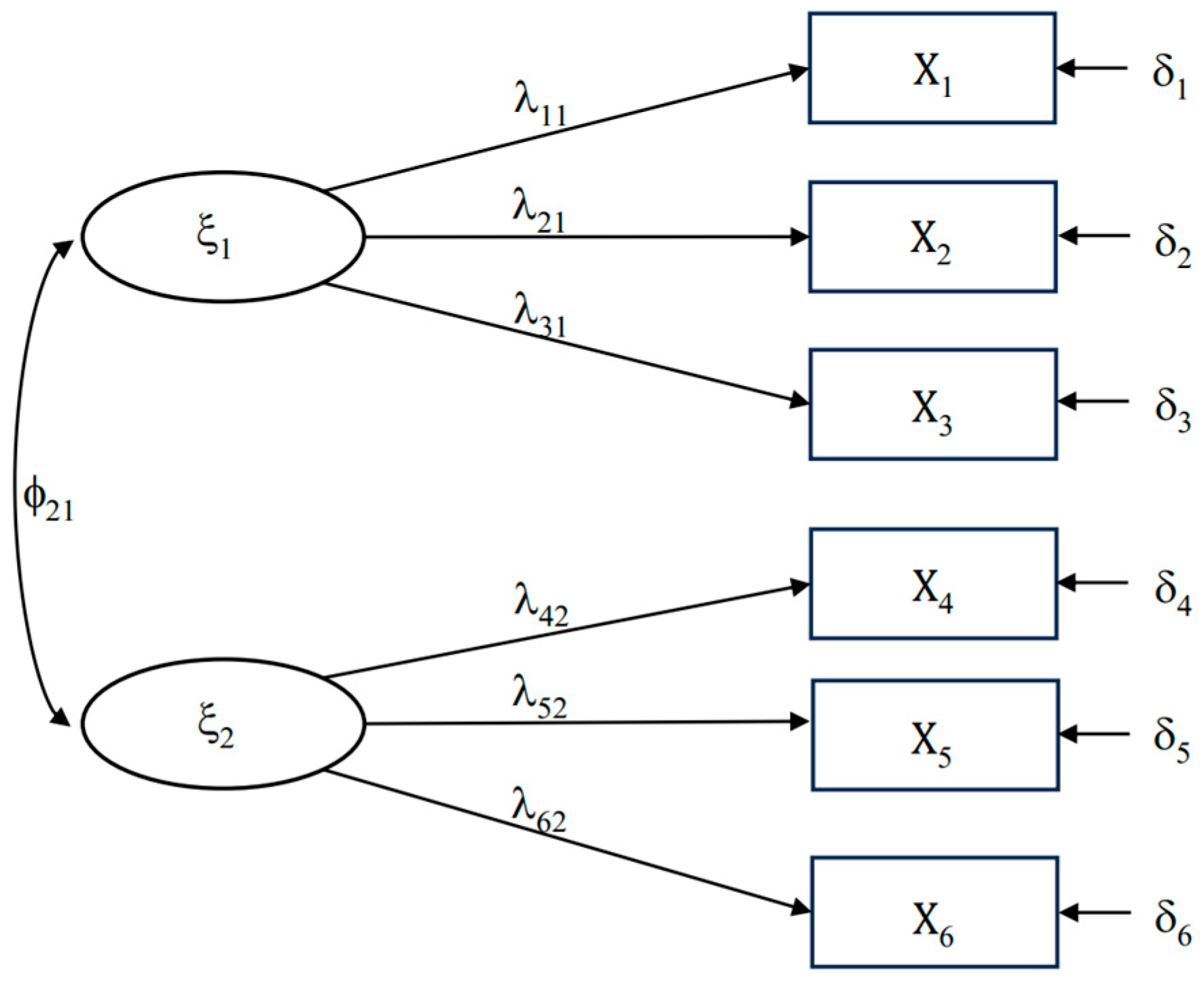
The structural equation model (SEM) considered (Figure 1) is described by the equation
where is the k-observed variables vector, is the n-latent variables vector, is the k-residual terms vector and is the matrix of factor loadings. It is assumed that
The variance–covariance matrix of the model is given by
where is the variance-covariance matrix of the latent variables , and is the variance–covariance matrix of the residual terms (diagonal). The parameters of the model are the factor loadings and factor covariances and the variances of the residual terms are given by .
The estimation of a structural equation model consists in finding the parameter estimates that result in a variance–covariance matrix, S, that best reproduces the variance–covariance implicit to the theoretical model considered, ∑ [34]. This process uses a discrepancy function, a mathematical procedure that minimizes the difference between the matrices S and ∑. The most common adjustment function is that obtained by the maximum-likelihood method [9]. If there are omissions in the data, the structural equation model estimation can be made using the FIML. In this estimation method, all the available information (all the cases) is used in the estimation process of model parameters and the standard errors, with some of the cases contributing more information than others [5,35]. When the omission mechanism of the data is MCAR, and the data have a normal multivariate distribution, the FIML method produces consistent and efficient parameter estimates, standard errors and statistical tests [5].
Another, procedure for handling missing data is MI. In this approach, values are assigned to missing observations. This procedure consists of three steps: a first imputation step where the omissions are imputed with m different values, an analysis step where the model is adjusted for each of the m datasets and a final step where the m results obtained in the previous step are combined. Contrary to the FIML method, it is quite computationally demanding, particularly in the imputation phase [5].
It should be noted that an SEM is composed by the measurement model and the structural model. A measurement model examines the relationship between latent variables and the observed variables. The structural model examines the relationship between the latent variables. In this work, a measurement model (Figure 1) is considered. This type of model is particularly important for the study of a multidimensional concept or for the development of a scale in psychology or education studies [36,37,38].
2.3. Fit Measures
The quantification of the adjustment of an SEM is very important and can be performed using some different indices, which are based in distinct criteria to identify the best model [39]. Although many fit indices are available for this purpose, the most used with this type of modeling are the RMSEA, the SRMR, the CFI and the TLI. In contrast, the behavior of these fit indices has been analyzed in other simulation studies with other conditions [13,14,40,41,42,43]. Most researchers agree that more than one fit index should be used to assure confidence in the model fit [8,9]. Given the frequent use of these fit indices, it is important to understand how they perform when used with models with nonresponses imposed by the researcher.
The RMSEA [44] is an absolute fit index. This type of index assesses the differences between S and ∑ and is considered the most direct form of assessment of how suitable the theoretical model fits the sample data [9]. Lower values represent a better fit, with RMSEA < 0.05 being considered a good fit. Nevertheless, values under 0.08 are acceptable [45,46].
The RMSEA is given by
where F is the minimum value of the discrepancy function.
Similarly, the SRMR [47] is also an absolute fit index and is given by
where is a component of the sample matrix S, is a component of the theoretical model matrix ∑ and p is the number of observed variables. The SRMR ranges between 0 and 1, with lower values indicating better fitting [48]. When SRMR < 0.05, it can be interpreted as a good fit.
The CFI [49] is an incremental fit index, which compares the postulated model with a more restricted baseline model [9]. Typically, this model has all correlations between observed variables set to zero and is called the null model.
The CFI index is given by
where and represent the chi-square statistic and the degrees of freedom for the baseline model, respectively. The and denote the chi-square statistic and degrees of freedom for the postulated model, respectively. The CFI index take values between 0 and 1, with higher values indicating a better fit. The fit of the model is considered good when CFI ≥ 0.95 [45].
The TLI [50] is also an incremental fit index and is given by
2.4. Simulation Conditions
The current research explores the effect of the nonresponses due to a specific planned missing design, the 3-form design, on the structural equation models fit indices CFI, TLI, RMSEA and SRMR. The simulation conditions were obtained by manipulating five variables: sample size, model size, factor loadings and correlation between factors, in an SEM model with two factors. Three different sample sizes are considered with 200, 500 and 1000 observations (small, medium, and large, respectively), values like those found in [6,11,12]. Model size refers to the total number of observed variables in the model, and 18 and 36 indicators (medium and large number of indicators) have been considered because, according to Jackson and colleagues [51], the medium number of indicators considered in the models is 17. I also consider an SEM with two factors, as performed by Muthén and Muthén [52], Madson and colleagues [53], Derby and Smith [54], Meng and colleagues [37] and In’nami and colleagues [38] (an example with six observed variables is presented in Figure 1). For the factor loadings the values 0.4 and 0.8 (low and high values) are considered, which are similar values to those found in Iacobucci [12], McNeish and colleagues [55], Schumacher and Lomax [11] and Shi and colleagues [14]. These authors considered factor loading values between 0.3 and 0.9. The correlation between factors was 0.1 and 0.9 (a weak and a strong association). I also consider a model misspecification in the correlation between factors as Fitzgerald and colleagues [16] or Shi and colleagues [14] assumed. The parameters were randomly drawn from a uniform distribution, with boundaries of 0.05 and 0.15 for weak correlation and 0.85 and 0.95 for strong correlation. For more about model misspecification with SEM, see the work of Robitzsch [56].
Datasets with complete observations and with nonresponses according to a 3-form design are generated. The percentage of missing data is maintained equally in all the generated databases, regardless the number of indicators in the model, and is the same as that used by Schoemann and colleagues [22]. In Table 2, I present the planned missing designs generated with a SEM with two factors. The omissions were generated for indicators in both factors.
A total of 1000 replications was generated considering all the possible combinations between the manipulated variables with complete and missing data. The nonresponses under analysis result from a 3-form design. The number of replications considered is as in McNeish and colleagues [55] or Schoemann and colleagues [22].
This simulation study was performed with the package simsem in R [23]. It allows the variation of parameter values and model misspecification across parameters. It is also possible to impose missing data in the simulated data and easily summarize results from simulations afterwards. For handling missing data, the FIML method is the default option, which was used in this work.
3. Results
The obtained results of the proposed simulation work are presented in Table 3, Table 4, Table 5 and Table 6. All of them present the mean value of the indices of interest obtained from the 1000 replications, from which it is possible to conclude that, when the sample size increases, all the indices present better values: CFI and TLI increase and SRMR and RMSEA decrease. In general, the results are worst with nonresponses when considering a misspecified models versus correctly specified models.
In Table 3, I present the obtained CFI values. With low factor loadings (0.4) and small sample size (200), it is possible to see that the CFI values are below the cutoff when there are missing data. In big models, even with complete data the obtained, the CFI value is under the acceptable (0.933). If the factor loadings are high (0.8), the CFI values obtained are acceptable despite the existence of nonresponses.
The CFI values for models with strong correlation between factors (0.9) show that nonresponses in correctly specified models causes values to be below the cutoff (0.942), in big models (36 indicators) with low factor loadings (0.4) and small samples. Independently of the factor loading values or sample size, omissions in models with misspecification causes unacceptable CFI values. The worst results are for models with low factor loadings and medium number of indicators, when this index takes values of 0.706, 0.724 and 0.726, according to the different samples sizes (200, 500 and 1000).
In Table 4, I show the obtained results for the TLI index. When a weak correlation between factors is considered, the existence of nonresponses causes TLI values to be below the cutoff in large models (36 indicators) with factor loadings equal to 0.4 and small sample sizes. Even with complete data, the obtained value is under the acceptable (0.932). For models with strong correlation between factors, the existence of omissions in models with misspecification leads to bad TLI values (below the desirable), whatever the factor loading values, model size or sample size are. TLI lowers with smaller factor loading values. The worst situation happens when the factor loadings are low and the model is of medium size (18 indicators), taking the values 0.666, 0.687 and 0.690, according to sample dimension.
When analyzing Table 5, in small samples with low factor loadings and weak correlation, the SRMR values are above 0.05 with both complete and missing data in correctly or misspecified models. With factor loading value of 0.8 and small and medium sample sizes, only when there are omissions with misspecified models, the SRMR index takes values above the acceptable, although the obtained values are worse in larger models. The results of SRMR index for models with strong correlation between factors show that the existence of omissions in correctly specified models only causes unacceptable values when the sample is small. However, if there are omissions when considering misspecified models, regardless of the sample size or the model size, the SRMR index values are far above the acceptable. If factor loadings are high, the existence of nonresponses with misspecified models causes the index’s values to be much higher than 0.05. The worst situation happens when a big model is considered, with the values lying around 0.392.
The obtained values for RMSEA index are presented in Table 6. When in the presence of a medium sized model with low factor loadings and a strong correlation between factors, this index presents values above the cutoff if there are nonresponses with misspecified models, regardless the sample size. Also, with high factor loadings and models of medium size, RMSEA values are unacceptable, around 0.097. If the model is of big size and small sample size the obtained result is 0.056, slightly above the desirable.
4. Discussion
This study explores the effect of nonresponses in the most popular fit measures of a structural equation model. Missing data are generated according a three-form design, in which the nonresponses are due to the will of the researcher. The purpose of using such a design is to increase the quality of the data, avoiding the effort of inquiry and the consequent non-response. However, there is low usage of this type of design, according to Enders [5], “Planned missing designs are highly useful and underutilized tools that will undoubtedly increase in popularity in the future”. Another procedure presented in psychology or marketing studies, to avoid nonresponses, is the forced answer options. However, the costs of the effect of using this method in terms of quality reduction and dropout rate may be high.
Also, in this study, I considered correctly specified and misspecified models with misspecification in the correlation between factors, as in the works of Shi and colleagues [14], Fitzgerald and colleagues [16], McNeisch and colleagues [55].
The findings regarding the effects of this type of missing values on the RMSEA index, only show values above the cutoff, when the correlation between factors is strong in misspecified models with high factor loadings and medium sized models, or in small samples with large models. The RMSEA index did not show to be affected by nonresponses in correctly specified models, which has been noted by Davey [57] and Hoyle [58]. In their work, Zhang and Savalei [59] explored the existence of a bias in the RMSEA values, concluding that factors such as the missing data mechanism and the type of misspecification are determinant for it. Recently, Fitzgeral and colleagues [16] proposed a correction for the RMSEA index to overcome this issue. The work of Lai [21] follows the same purpose.
The SRMR values showed this index to be affected by nonresponses, particularly with small samples, low factor loadings and with medium and large number of observed variables in the model. In these cases, it presents values above the cutoff, even for complete data. However, if a misspecified model with data from a three-form design in small samples is considered, the SRMR values are the worst. With high factor loadings, even with medium and large samples, the SRMR is above the acceptable. As stated by Jia and colleagues [6], when using a planned missing design, it is not simply that a larger sample is better, it depends on the other conditions of the study.
The CFI index is affected by a three-form design, particularly, with small samples, low factor loadings and high number of observed variables (large models). In this case, it presents values under the cutoff, even for complete data. As presented by Shi and colleagues [14], CFI showed to be affected by the size of the model when data from a three-form design are considered. If there is a misspecification in the correlation between factors, the CFI index presents unacceptable values, despite the sample and model size as well as the factor loadings assumed. Zhang and Savalei [18,59] point the use of the estimation method FIML for handling missing data as the cause of the distortion in CFI and RMSEA values.
For all the considered indices, a larger number of observed variables in the model causes worse values, lower for the CFI index and higher for the RMSEA and SRMR indices. Additionally, models with low factor loadings have worse values for the considered fit indices. These results for all the four indices are in line with the work of Shi and colleagues [14]. According to these authors, small sample sizes, high number of observed variables in the model and lower factor loadings lead to a worse fit. In the same sense is the work of Moshagen [60], which shows the effect of the sample size and model size on the fit indices.
When factor loading values are low, in small samples, the obtained SRMR and CFI values suggest a weak fit model-data. According to McNeish and colleagues [55] and Hancock and Mueller [61], there is another measure that is important to pay attention to when performing a study, measurement quality, considered as the strength of the standardized factor loadings by the authors. In McNeish and colleagues [55] work, they show the large influence measurement quality (factor loadings values) has on fit indices values and how greatly the cutoffs would change if they were derived under an alternative level of measurement quality. They highlight the fact that the cutoffs established by Hu and Bentler [45] are derived from models, most of them with factor loading values of 0.7 and a few with 0.75 or 0.80, considered high values for factor loadings. So, the findings of this study do not seem to be aligned with the reliability paradox presented by Hancock and Mueller [61].
The indices CFI, TLI and RMSEA are affected in the same way by a three-form design, when the correlation between factors is weak, regardless of the model being or not correctly specified. However, for the SRMR index, this only happens with low factor loadings. According to Themessl-Huber [62], all statistics have problems detecting misspecified models when factor loadings are low. These findings in models with low factor loadings are particularly important, as in psychology, where studies are performed with a mean value for factor loadings, according to Peterson [63], of 0.32. As such, there is the need to look to all the assumptions of the study, as suggested by Jia and colleagues [6]. When the correlation is strong, all the indices are affected by the model misspecification, regardless of sample size.
Considering large sample sizes, with data from a three-form design, for different models and parameter values, all the four fit measures did not appear to be affected as they all presented acceptable fit values (good fit) in correctly specified models. Furthermore, the RMSEA, TLI and CFI indices presented similar results with complete and missing data, whereas the same does not happen with the SRMR index. In the study of Cangur and Ercan [15], with complete data, the SRMR show to be the index with worst performance. As in the work of Fan, Thompson and Wang [64], all the fit indices showed to be affected by the sample size, particularly by small samples.
On the other hand, it was possible to see that the number of indicators in the model (model size) impacts the fit measures, particularly, CFI, TLI and SRMR, as stated by Shi and colleagues [14], when considering misspecified models. For RMSEA the effect is the opposite to that stated in the work of these authors.
This work has some limitations that can be further improved. The findings are based on a particular three-form design, as presented by Schoemann and colleagues [22]. This three-form design has a specific number of variables in each set X, A, B and C, resulting in a percentage of missing data in the data base of approximately 11.1%, and, despite the number of indicators considered in the model, this percentage was maintained so the results are comparable. In future works, it would be interesting to increase the percentage of nonresponses by manipulating the number of indicators in each set of variables and considering ordinal missing data.
Considering the two-method suggested by Graham [1], it would also be interesting and valuable to compare the obtained values, because the study of omissions by design has been underestimated, particularly with misspecified models.
Finally, considering other structural equation models frequently used in psychology studies and understanding the behavior of the fit measures when the data present omissions by design is also challenging.
5. Conclusions
The present work aims to help applied researchers that are using structural equation models with data obtained from a particular planned missing design, a three-form design. The later design allows us to reduce the number of questions in a survey that each participant answered without reducing the overall number of questions in the survey. Consequently, this reduces the time and burden needed to complete each survey, improving the quality and the quantity of the obtained responses. They are particularly important in psychological research, where time and resources are limited. However, is important to understand the consequences of using such a design in the usual fit measures considered in the evaluation of the adjustment of a SEM.
The results obtained in the current study showed that for small samples, TLI and CFI have a similar behavior with omissions from a three-form design with correctly and misspecified models. They have worse values with a strong correlation between factors despite the model size and the factor loading values. The SRMR index is affected by a three-form design with correctly specified models when the factor loadings are low and if the factor loadings are high in misspecified models. The RMSEA index shows a bad fit only if it considers misspecified models with strong correlation between factors.
All the four fit measures did not appear to be affected for the existence of nonresponses from a three-form design, and all of them presented acceptable fit values (good fit) with correctly specified models when considering large sample sizes despite different models or parameter values. However, the existence of a model misspecification leads to worse values for the fit measures, particularly when there is a strong correlation between factors.
The obtained results highlight the necessity of considering nonresponse patterns during model fitting with misspecified models and factors with strong correlations.
Funding
This research received no external funding.
Data Availability Statement
Codes to generate and analyze the data will be made available upon reasonable request by contacting the corresponding author.
Conflicts of Interest
The author declares no conflict of interest.
References
- Graham, J.; Taylor, B.; Olchowski, A.; Cumsville, P. Planned missing data designs in psychological research. Psychol. Methods 2006, 11, 323–343. [Google Scholar] [CrossRef]
- Graham, J.; Hofer, S.; Mackinnon, D. Maximizing the usefulness of data obtained with planned missing value patterns: An application of maximum likelihood procedures. Multivar. Behav. Res. 1996, 31, 197–218. [Google Scholar] [CrossRef] [PubMed]
- McArdle, J.J. Structural factor analysis experiments with incomplete data. Multivar. Behav. Res. 1994, 29, 409–454. [Google Scholar] [CrossRef] [PubMed]
- Raghunathan, T.; Grizzle, J. A Split Questionnaire Survey Design. J. Am. Stat. Assoc. 1995, 90, 54–63. [Google Scholar] [CrossRef]
- Enders, C.K. Applied Missing Data; The Guilford Press: New York, NY, USA, 2010; pp. 21–36. [Google Scholar]
- Jia, F.; Moore, E.W.G.; Kinai, R.; Crowe, K.S.; Schoemann, A.M.; Little, T. Planned missing data designs with small sample sizes: How small is too small? Int. J. Behav. Dev. 2014, 38, 435–452. [Google Scholar] [CrossRef]
- Moore, E.W.G.; Lang, K.M.; Grandfield, E.M. Maximizing data quality and shortening survey time: Three-form planned missing data survey design. Psychol. Sport Exerc. 2020, 51, 1–12. [Google Scholar] [CrossRef]
- Bandalous, D.L.; Finney, S.J. Factor analysis: Exploratory and confirmatory. In The Reviewer’s Guide to Quantitative Methods in the Social Sciences; Hancock, G.R., Mueller, R.O., Eds.; Routledge: New York, NY, USA, 2010; pp. 109–130. [Google Scholar] [CrossRef]
- Hair, J.F.; Black, W.C.; Babin, B.J.; Anderson, R.E.; Tatham, R.L. Multivariate Data Analysis, 6th ed.; Pearson: Columbus, OH, USA, 2006; pp. 426–461. [Google Scholar]
- Nye, C.D. Reviewer Resources: Confirmatory Factor Analysis. Organ. Res. Methods 2022. online publishing. [Google Scholar] [CrossRef]
- Schumacker, R.E.; Lomax, R.G. A Beginner’s Guide to Structural Equation Modelling, 3rd ed.; Routledge/Taylor & Francis Group: New York, NY, USA, 2010. [Google Scholar]
- Iacobucci, D. Structural equation modelling: Fit indices, sample size, and advanced topics. J. Consum. Psychol. 2010, 20, 90–98. [Google Scholar] [CrossRef]
- Kenny, D.A.; McCoach, D.B. Effect of the number of variables on measures of fit in structural equation modelling. Struct. Equ. Model. 2003, 10, 333–351. [Google Scholar] [CrossRef]
- Shi, D.; Lee, T.; Maydeu-Olivares, A. Understanding the Model Size Effect on SEM Fit Indices. Educ. Psychol. Meas. 2019, 79, 310–334. [Google Scholar] [CrossRef]
- Cangur, S.; Ercan, I. Comparison of model Fit Indices Used in Structural Equation Modeling Under Multivariate Normality. J. Mod. Appl. Stat. Methods 2015, 14, 152–167. [Google Scholar] [CrossRef]
- Fitzgerald, C.A.; Estabrook, R.; Martin, D.P.; Brandmaier, A.M.; von Oertzen, T. Correcting the Bias of the Root Mean Squared Error of Approximation under Missing Data. Methodology 2021, 17, 189–204. [Google Scholar] [CrossRef]
- Maydeu-Olivares, A. Assessing the size of model misfit in structural equation models. Psychometrika 2017, 82, 533–558. [Google Scholar] [CrossRef] [PubMed]
- Zhang, X.; Savalei, V. New computations for RMSEA and CFI following FIML and TS estimation with missing data. Psychol. Methods 2023, 28, 263–283. [Google Scholar] [CrossRef] [PubMed]
- Liu, Y.; Sriutaisuk, S. Evaluation of Model Fit in Structural Equation Models with Ordinal Missing Data: An examination of the D 2 Method. Struct. Equ. Model. Multidiscip. J. 2020, 27, 561–583. [Google Scholar] [CrossRef]
- Liu, Y.; Sriutaisuk, S.; Chung, S. Evaluation of model fit in structural equation models with ordinal missing data: A comparison of the D 2 and MI2S methods. Struct. Equ. Model. Multidiscip. J. 2021, 28, 740–762. [Google Scholar] [CrossRef]
- Lai, K. Correct estimation methods for RMSEA under missing data. Struct. Equ. Model. Multidiscip. J. 2021, 28, 207–218. [Google Scholar] [CrossRef]
- Schoemann, A.M.; Miller, P.; Pornprasertmanit, S.; Wu, W. Using Monte Carlo simulations to determine power and sample size for planned missing designs. Int. J. Behav. Dev. 2014, 38, 471–479. [Google Scholar] [CrossRef]
- Pornprasertmanit, S.; Miller, P.; Schoemann, A.; Jorgensen, T.D. Simsem: SIMulated Structural Equation Modeling (Version 0.5-16) [R Package]. 2021. Available online: http://simsem.org/ (accessed on 1 July 2022).
- Azar, B. Finding a solution for missing data. Monit. Psychol. 2002, 33, 70. [Google Scholar]
- Peugh, J.L.; Enders, K. Missing data in educational research: A review of reporting practices and suggestions for improvement. Rev. Educ. Res. 2004, 74, 525–556. [Google Scholar] [CrossRef]
- Albaum, G.; Roster, C.A.; Wiley, J.; Rossiter, J.; Smith, S.M. Designing web surveys in marketing research: Does use of forced answering affect completion rates? J. Mark. Theory Pract. 2010, 18, 285–294. [Google Scholar] [CrossRef]
- Roster, C.A.; Albaum, G.; Smith, S.M. Topic sensitivity and Internet survey design: A cross-cultural/national study. J. Mark. Theory Pract. 2014, 22, 91–102. [Google Scholar] [CrossRef]
- De Leeuw, E.D.; Hox, J.J.; Boevé, A. Handling Do-Not-Know Answers: Exploring New Approaches in Online and Mixed-Mode Surveys. Soc. Sci. Comput. Rev. 2016, 34, 116–132. [Google Scholar] [CrossRef]
- Décieux, J.P.; Mergener, A.; Neufang, K.M.; Sischka, P. Implementation of the forced answering option within online surveys: Do higher item response rates come at the expense of participation and answer quality? Psihologija 2015, 48, 311–326. [Google Scholar] [CrossRef]
- Steijer, S.; Reips, U.-D.; Voracek, M. Forced-response in online surveys: Bias from reactance and an increase in sex-specific dropout. J. Am. Soc. Inf. Sci. Technol. 2007, 58, 1653–1660. [Google Scholar] [CrossRef]
- Sischka, P.; Décieux, J.P.; Mergener, A.; Neufang, K.M.; Schmidt, A.F. The Impact of Forced Answering and Reactance on Answering Behavior in Online Surveys. Soc. Sci. Comput. Rev. 2020, 40, 405–425. [Google Scholar] [CrossRef]
- Little, R.J.A.; Rubin, D.B. Statistical Analysis with Missing Data, 2nd ed.; Wiley: Hoboken, NJ, USA, 2002. [Google Scholar] [CrossRef]
- Graham, J.; Hofer, S.; Piccinin, A.M. Analysis with missing data in drug prevention research. In Advances in Data Analysis for Prevention Intervention Research; National Institute on Drug Abuse Research Monograph Series; Collins, L.M., Seitz, L., Eds.; National Institute on Drug Abuse: Washington, DC, USA, 1994; Volume 142, pp. 13–63. [Google Scholar] [CrossRef]
- Bollen, K. Structural Equations with Latent Variables; Wiley: New York, NY, USA, 1989; pp. 80–116, 179–223. [Google Scholar]
- Arbuckle, J.L. Full information estimation in the presence of incomplete data. In Advanced Structural Equation Modelling; Marcoulides, G.A., Schumacker, R.E., Eds.; Lawrence Erlbaum Associates: Mahwah, NJ, USA, 1996; pp. 243–277. [Google Scholar]
- Golaszewski, N.M.; Bartholomew, J.B. The development of the Physical Activity and Social Support Scale. J. Sport Exerc. Psychol. 2019, 41, 215–229. [Google Scholar] [CrossRef]
- Meng, M.; He, J.; Guan, Y.; Zhao, H.; Yi, J.; Yae, S.; Li, L. Factorial Invariance of the 10-item Connor-Davidson Resilience Scale Across Gender Among Chinese Elders. Front. Psychol. 2019, 10. [Google Scholar] [CrossRef]
- In’nami, Y.; Koizumi, R. Factor Structure of the revised TOEIC® test: A multi-sample analysis. Lang. Test. 2021, 29, 131–152. [Google Scholar] [CrossRef]
- Yuan, K.-H. Fit indices versus test statistics. Multivar. Behav. Res. 2005, 40, 115–148. [Google Scholar] [CrossRef]
- Kenny, D.A.; Kanishan, B.; McCoach, D.B. The performance of RMSEA in models with small degrees of freedom. Sociol. Methods Res. 2015, 44, 486–507. [Google Scholar] [CrossRef]
- Maydeu-Olivares, A. Maximum likelihood estimation of structural equation models for continuous data: Standard errors and goodness of fit. Struct. Equ. Model. 2017, 24, 383–394. [Google Scholar] [CrossRef]
- Maydeu-Olivares, A.; Shi, D.; Rosseel, Y. Assessing fit in structural equation models: A Monte-Carlo evaluation of RMSEA versus SRMR confidence intervals and tests of close fit. Struct. Equ. Model. 2018, 25, 389–402. [Google Scholar] [CrossRef]
- Savalei, V. The relationship between root mean square error of approximation and model misspecification in confirmatory factor analysis models. Educ. Psychol. Meas. 2012, 72, 910–932. [Google Scholar] [CrossRef]
- Steiger, J.H. Structural model evaluation and modification: An interval estimation approach. Multivar. Behav. Res. 1990, 25, 173–180. [Google Scholar] [CrossRef] [PubMed]
- Hu, L.; Bentler, P.M. Cutoff criteria for fit indices in covariance structure analysis: Conventional criteria versus new alternatives. Struct. Equ. Model. 1999, 6, 1–55. [Google Scholar] [CrossRef]
- Kaplan, D. Structural Equation Modeling—Foundations and Extensions; Sage Publications: Madison, WI, USA, 2009; pp. 112–120. [Google Scholar] [CrossRef]
- Jöreskog, K.G.; Sörbom, D. LISREL VI: Analysis of Linear Structural Relationship by Maximum Likelihood and Least Squares Methods; National Educational Resources: Chicago, IL, USA, 1981; Available online: https://ssicentral.com/ (accessed on 1 July 2022).
- Kline, R.B. Principles and Practice of Structural Equation Modeling, 5th ed.; Guilford Press: New York, NY, USA, 2023; Chapter 10; pp. 156–180. [Google Scholar]
- Bentler, P.M. Comparative Fit Indices in Structural Equation Models. Psychol. Bull. 1990, 107, 238–246. [Google Scholar] [CrossRef]
- Tucker, L.R.; Lewis, C. The reliability coefficient for maximum likelihood factor analysis. Psychometrika 1973, 38, 1–10. [Google Scholar] [CrossRef]
- Jackson, D.L.; Gillaspy, J.A.; Purc-Stephenson, R. Reporting practices in confirmatory factor analysis: An overview and some recommendations. Psychol. Methods 2009, 14, 6–23. [Google Scholar] [CrossRef]
- Muthén, L.K.; Muthén, B.O. How to use a Monte Carlo Study to decide on sampled Size and Determine Power. Struct. Equ. Model. Multidiscip. J. 2002, 9, 599–620. [Google Scholar] [CrossRef]
- Madson, M.B.; Mohn, R.S.; Schumacher, J.A.; Landry, A.S. Measuring client experiences of motivational interviewing during a lifestyle intervention. Meas. Eval. Couns. Dev. 2015, 48, 140–151. [Google Scholar] [CrossRef] [PubMed]
- Derby, D.C.; Smith, T.J. Exploring the factorial structure for behavioural consequences of college student drinking. Meas. Eval. Couns. Dev. 2008, 41, 32–41. [Google Scholar] [CrossRef]
- McNeish, D.; An, J.; Hancock, G.R. The Thorny Relation Between Measurement Quality and Fit Index Cutoffs in Latent Variable Models. J. Person. Assess. 2018, 100, 43–52. [Google Scholar] [CrossRef] [PubMed]
- Robitzch, A. Modeling Model Misspecification in Structural Equation Models. Stats 2023, 6, 689–705. [Google Scholar] [CrossRef]
- Davey, A. Issues in evaluating model fit with missing data. Struct. Equ. Model. Multidiscip. J. 2005, 12, 578–597. [Google Scholar] [CrossRef]
- Hoyle, R.H. Handbook of Structural Equation Modelling; Guilford Press: New York, NY, USA, 2012. [Google Scholar]
- Zhang, X.; Savalei, V. Examining the effect of missing data on RMSEA and CFI under normal theory full-information maximum likelihood. Struct. Equ. Model. Multidiscip. J. 2020, 27, 219–239. [Google Scholar] [CrossRef]
- Moshagen, M. The model size effect in SEM: Inflated goodness-of-fit statistics are due to the size of the covariance matrix. Struct. Equ. Model. Multidiscip. J. 2012, 19, 86–98. [Google Scholar] [CrossRef]
- Hancock, G.R.; Mueller, R.O. The reliability paradox in assessing structural relations within covariance structure models. Educ. Psychol. Meas. 2011, 71, 306–324. [Google Scholar] [CrossRef]
- Themessl-Huber, M. Evaluation of the χ2-statistic and different fit-indices under misspecified number of factors in confirmatory factor analysis. Psychol. Test Assess. Model. 2014, 56, 219–236. [Google Scholar]
- Peterson, R.A. A meta-analysis of variance accounted for and factor loadings in exploratory factor analysis. Mark. Lett. 2000, 11, 261–275. [Google Scholar] [CrossRef]
- Fan, X.; Thompson, B.; Wang, L. Effects of sample size, estimation methods, and model specification on structural equation modeling fit indexes. Struct. Equ. Model. Multidiscip. J. 1999, 6, 56–83. [Google Scholar] [CrossRef]
Figure 1.
Structural equation model with two factors and six observed variables (three in each factor).
Figure 1.
Structural equation model with two factors and six observed variables (three in each factor).


Table 1.
The three-form design: O—observed value, NA—not available.
| Question Set | ||||
|---|---|---|---|---|
| Form | X | A | B | C |
| 1 | O | O | O | NA |
| 2 | O | O | NA | O |
| 3 | O | NA | O | O |
Table 2.
Variables considered in each of the groups: X, A, B and C of the 3-form design when considered a model with two factors.
Table 2.
Variables considered in each of the groups: X, A, B and C of the 3-form design when considered a model with two factors.
| Number of Indicators in the Model | Questions in Each Set | |||
|---|---|---|---|---|
| X | A | B | C | |
| 18 | 1, 2, 3, 4, 6, 8, 10, 11, 12, 14, 16, 18 | 5, 13 | 7, 15 | 9, 17 |
| 36 | 1, 2, 3, 4, 7, 8, 9, 10, 13, 14, 15, 16, 19, 20, 23, 24, 25, 26, 29, 30, 31, 32, 35, 36 | 5, 6, 21, 22 | 11, 12, 27, 28 | 17, 18, 33, 34 |
Table 3.
CFI values for different sample sizes, complete data, data from a 3-form and data from a 3-form with a misspecified model. Model with 18 and 36 indicators, factor loadings 0.4 and 0.8, correlation between factors 0.1 and 0.9.
Table 3.
CFI values for different sample sizes, complete data, data from a 3-form and data from a 3-form with a misspecified model. Model with 18 and 36 indicators, factor loadings 0.4 and 0.8, correlation between factors 0.1 and 0.9.
| Number of Indicators | CFI | |||||||
|---|---|---|---|---|---|---|---|---|
| 18 | 36 | |||||||
| Correlation | Factor Loading | Sample Size | Complete | 3-Form | 3-Form+ Misspec | Complete | 3-Form | 3-Form+ Misspec |
| 0.1 | 0.4 | 200 | 0.964 | 0.944 | 0.942 | 0.933 | 0.878 | 0.872 |
| 500 | 0.986 | 0.982 | 0.980 | 0.986 | 0.978 | 0.977 | ||
| 1000 | 0.994 | 0.992 | 0.990 | 0.995 | 0.993 | 0.991 | ||
| 0.8 | 200 | 0.996 | 0.995 | 0.994 | 0.992 | 0.984 | 0.984 | |
| 500 | 0.999 | 0.998 | 0.998 | 0.998 | 0.998 | 0.997 | ||
| 1000 | 0.999 | 0.999 | 0.999 | 0.999 | 0.999 | 0.999 | ||
| 0.9 | 0.4 | 200 | 0.971 | 0.958 | 0.706 | 0.942 | 0.895 | 0.733 |
| 500 | 0.990 | 0.987 | 0.724 | 0.988 | 0.982 | 0.806 | ||
| 1000 | 0.995 | 0.994 | 0.726 | 0.996 | 0.994 | 0.816 | ||
| 0.8 | 200 | 0.997 | 0.995 | 0.894 | 0.992 | 0.995 | 0.934 | |
| 500 | 0.999 | 0.999 | 0.897 | 0.998 | 0.999 | 0.946 | ||
| 1000 | 0.999 | 0.999 | 0.897 | 0.999 | 0.999 | 0.947 | ||
Table 4.
TLI values for different sample sizes, complete data, data from a 3-form and data from a 3-form with a misspecified model. Model with 18 and 36 indicators, factor loadings 0.4 and 0.8, correlation between factors 0.1 and 0.9.
Table 4.
TLI values for different sample sizes, complete data, data from a 3-form and data from a 3-form with a misspecified model. Model with 18 and 36 indicators, factor loadings 0.4 and 0.8, correlation between factors 0.1 and 0.9.
| Number of Indicators | TLI | |||||||
|---|---|---|---|---|---|---|---|---|
| 18 | 36 | |||||||
| Correlation | Factor Loading | Sample Size | Complete | 3-Form | 3-Form+ Misspec | Complete | 3-Form | 3-Form+ Misspec |
| 0.1 | 0.4 | 200 | 0.983 | 0.959 | 0.955 | 0.932 | 0.871 | 0.864 |
| 500 | 0.996 | 0.993 | 0.988 | 0.989 | 0.980 | 0.978 | ||
| 1000 | 0.999 | 0.998 | 0.994 | 0.998 | 0.996 | 1.000 | ||
| 0.8 | 200 | 0.998 | 0.996 | 0.995 | 0.992 | 0.983 | 0.984 | |
| 500 | 1.000 | 0.999 | 0.998 | 0.999 | 0.998 | 0.997 | ||
| 1000 | 1.000 | 1.000 | 0.999 | 1.000 | 1.000 | 1.000 | ||
| 0.9 | 0.4 | 200 | 0.986 | 0.969 | 0.666 | 0.942 | 0.889 | 0.717 |
| 500 | 0.998 | 0.995 | 0.687 | 0.991 | 0.984 | 0.794 | ||
| 1000 | 0.999 | 0.999 | 0.690 | 0.998 | 0.997 | 0.804 | ||
| 0.8 | 200 | 0.998 | 0.996 | 0.880 | 0.992 | 0.985 | 0.930 | |
| 500 | 1.000 | 0.999 | 0.883 | 0.999 | 0.998 | 0.942 | ||
| 1000 | 1.000 | 1.000 | 0.884 | 1.000 | 1.000 | 0.944 | ||
Table 5.
SRMR values for different sample sizes, complete data and data from a 3-form and data from a 3-form with a misspecified model. Model with 18 and 36 indicators, factor loadings 0.4 and 0.8, correlation between factors 0.1 and 0.9.
Table 5.
SRMR values for different sample sizes, complete data and data from a 3-form and data from a 3-form with a misspecified model. Model with 18 and 36 indicators, factor loadings 0.4 and 0.8, correlation between factors 0.1 and 0.9.
| Number of Indicators | SRMR | |||||||
|---|---|---|---|---|---|---|---|---|
| 18 | 36 | |||||||
| Correlation | Factor Loading | Sample Size | Complete | 3-Form | 3-Form+ Misspec | Complete | 3-Form | 3-Form+ Misspec |
| 0.1 | 0.4 | 200 | 0.055 | 0.067 | 0.069 | 0.060 | 0.075 | 0.077 |
| 500 | 0.035 | 0.042 | 0.044 | 0.038 | 0.045 | 0.047 | ||
| 1000 | 0.024 | 0.029 | 0.032 | 0.027 | 0.032 | 0.033 | ||
| 0.8 | 200 | 0.036 | 0.043 | 0.065 | 0.039 | 0.048 | 0.070 | |
| 500 | 0.023 | 0.026 | 0.052 | 0.025 | 0.029 | 0.055 | ||
| 1000 | 0.016 | 0.019 | 0.047 | 0.018 | 0.020 | 0.029 | ||
| 0.9 | 0.4 | 200 | 0.050 | 0.063 | 0.115 | 0.055 | 0.071 | 0.122 |
| 500 | 0.032 | 0.039 | 0.103 | 0.035 | 0.043 | 0.108 | ||
| 1000 | 0.023 | 0.027 | 0.099 | 0.025 | 0.030 | 0.103 | ||
| 0.8 | 200 | 0.024 | 0.031 | 0.378 | 0.027 | 0.036 | 0.392 | |
| 500 | 0.015 | 0.019 | 0.378 | 0.017 | 0.021 | 0.392 | ||
| 1000 | 0.011 | 0.013 | 0.370 | 0.012 | 0.014 | 0.392 | ||
Table 6.
RMSEA values for different sample sizes, complete data and data from a 3-form and data from a 3-form with a misspecified model. Model with 18 and 36 indicators, factor loadings 0.4 and 0.8, correlation between factors 0.1 and 0.9.
Table 6.
RMSEA values for different sample sizes, complete data and data from a 3-form and data from a 3-form with a misspecified model. Model with 18 and 36 indicators, factor loadings 0.4 and 0.8, correlation between factors 0.1 and 0.9.
| Number of Indicators | RMSEA | |||||||
|---|---|---|---|---|---|---|---|---|
| 18 | 36 | |||||||
| Correlation | Factor Loading | Sample Size | Complete | 3-Form | 3-Form+ Misspec | Complete | 3-Form | 3-Form+ Misspec |
| 0.1 | 0.4 | 200 | 0.013 | 0.016 | 0.016 | 0.018 | 0.025 | 0.026 |
| 500 | 0.007 | 0.008 | 0.009 | 0.007 | 0.008 | 0.009 | ||
| 1000 | 0.005 | 0.005 | 0.006 | 0.004 | 0.004 | 0.003 | ||
| 0.8 | 200 | 0.013 | 0.016 | 0.018 | 0.019 | 0.025 | 0.025 | |
| 500 | 0.007 | 0.008 | 0.010 | 0.007 | 0.008 | 0.009 | ||
| 1000 | 0.005 | 0.005 | 0.008 | 0.004 | 0.005 | 0.003 | ||
| 0.9 | 0.4 | 200 | 0.013 | 0.016 | 0.054 | 0.018 | 0.025 | 0.041 |
| 500 | 0.007 | 0.008 | 0.051 | 0.007 | 0.008 | 0.034 | ||
| 1000 | 0.005 | 0.005 | 0.051 | 0.004 | 0.004 | 0.033 | ||
| 0.8 | 200 | 0.014 | 0.016 | 0.097 | 0.018 | 0.025 | 0.056 | |
| 500 | 0.007 | 0.008 | 0.096 | 0.007 | 0.008 | 0.050 | ||
| 1000 | 0.005 | 0.005 | 0.096 | 0.004 | 0.004 | 0.049 | ||
Disclaimer/Publisher’s Note: The statements, opinions and data contained in all publications are solely those of the individual author(s) and contributor(s) and not of MDPI and/or the editor(s). MDPI and/or the editor(s) disclaim responsibility for any injury to people or property resulting from any ideas, methods, instructions or products referred to in the content. |
© 2023 by the author. Licensee MDPI, Basel, Switzerland. This article is an open access article distributed under the terms and conditions of the Creative Commons Attribution (CC BY) license (https://creativecommons.org/licenses/by/4.0/).
Share and Cite
MDPI and ACS Style
Vicente, P.C.R. Evaluating the Effect of Planned Missing Designs in Structural Equation Model Fit Measures. Psych 2023, 5, 983-995. https://doi.org/10.3390/psych5030064
AMA Style
Vicente PCR. Evaluating the Effect of Planned Missing Designs in Structural Equation Model Fit Measures. Psych. 2023; 5(3):983-995. https://doi.org/10.3390/psych5030064
Chicago/Turabian StyleVicente, Paula C. R. 2023. "Evaluating the Effect of Planned Missing Designs in Structural Equation Model Fit Measures" Psych 5, no. 3: 983-995. https://doi.org/10.3390/psych5030064