An Introduction to Factored Regression Models with Blimp

Abstract

In this paper, we provide an introduction to the factored regression framework. This modeling framework applies the rules of probability to break up or “factor” a complex joint distribution into a product of conditional regression models. Using this framework, we can easily specify the complex multivariate models that missing data modeling requires. The article provides a brief conceptual overview of factored regression and describes the functional notation used to conceptualize the models. Furthermore, we present a conceptual overview of how the models are estimated and imputations are obtained. Finally, we discuss how users can use the free software package, Blimp, to estimate the models in the context of a mediation example.

1. Introduction

In the missing data literature, there has been a consistent focus on breaking up complex multivariate distributions into more manageable conditional distributions. By applying rules of probability, we can take a joint density or distribution of two variables and break it up or “factored” it into the product of the conditional density multiplied by the marginal density. Ibrahim and colleagues [1,2,3] first introduced this approach, and the literature has referred to this specification as fully Bayesian estimation, sequential specification, or factored regression [4,5,6,7,8,9]. The factored regression approach simplifies many issues that arise when accounting for missing data, where we generally model the joint distribution of all missing variables and our outcomes to obtain unbiased estimates under assumptions of how the unobserved values came to be—e.g., missing at random [10].

This paper introduces how to specify factored regression models and apply them to estimate models with missing predictors and outcomes. We illustrate how we can leverage factored regression to obtain parameter estimates or produce multiple imputations, which are then used for subsequent analyses. Throughout the paper, we discuss using the Bayesian and imputation software package Blimp Version 3.0 [11] to estimate the models. Blimp is a free standalone software package that extends factored regression to a flexible latent variable modeling framework and can handle a wide array of missing response types, nonlinear relationships, and multilevel data structures common in psychological and social sciences. While we will focus on specifying the models with Blimp, several alternative R packages exist to specify similar statistical models—see mdmb, smcfcs, JointAI packages [12,13,14].

The structure of this paper is as follows. First, we provide a brief conceptual overview of factored regression and describe the functional notation we use throughout the article. Second, we illustrate the factored regression approach concretely by applying it to a three-variable moderated regression. Third, we briefly discuss the estimation of factor regression using Markov chain Monte Carlo techniques and obtain “imputations” for the missing observations—i.e., via data augmentation [15]. Fourth, we discuss the extension of factored regression to a path modeling framework using a single-mediator interaction model [16]. Fifth, we illustrate how the factored regression framework can be applied to include measurement models, where we illustrate how to specify a single-mediator interaction model with a latent by continuous interaction. Sixth, we illustrate how to estimate factor regression models using the freely available Blimp software package [11] via a substantive data example.

2. Factored Regression Modeling Framework

Conceptually, we can think of factored regression as chaining several regression models to characterize an entire joint distribution of variables. Some of these regression models will consist of relationships we are substantively interested in, while others will act as a tool to maintain the association between two variables that may not be of substantive interest. Throughout this paper, we will specify models in terms of a so-called functional notation. To illustrate, suppose we have the joint distribution of two variables, X and Y. A functional notation would represent the joint distribution as

$$f(X,Y),$$

where the $f(\dots )$ represents a general probability distribution for both X and Y. As mentioned above, we can break apart this distribution into two parts:

$$f(X,Y)=f(Y\mid X)f\left(X\right).$$

The first part, $f(Y\mid X)$, is the conditional distribution of Y given X. Said differently, this is a regression model where we are predicting Y from X. Notably, the form of this regression is unspecified; that is, the relationship could be linear, quadratic, logistic, or some more complex relationship. Thus, to specify a factored regression model, we first break up or “factor” a complicated joint distribution of variables into a product of less complicated, often conditional distributions via the functional notation. Second, we specify the form of each function, modeling the relationship between the criterion (variables left of the bar) and the regressors (variables right of the bar). By breaking up the joint distribution into manageable chunks, we are afforded more flexibility to model complex relationships such as interactions, nonlinearities, mixed response types, and clustered data. In contrast, a traditional linear structural equation modeling (SEM) framework generally requires multivariate normality on all endogenous and missing variables, precluding nonlinear relationships between missing predictors.

We will specify factor regressions in two steps. First, we will take the joint distribution of all variables and factor it into the product of several conditional distributions. Second, we specify the actual form or model for each function. Generally speaking, these models will specify the relationship between the criteria (variables left of the bar) and the regressors (variables right of the bar). In essence, we will break up the joint distribution into manageable chunks, and this affords us more flexibility to model complex relationships. In other words, it is easier to specify relationships conditionally given some variables as opposed to jointly. In contrast, a traditional structural equation modeling (SEM) framework generally requires us to consider multivariate normality for all endogenous and missing variables, and this requirement precludes nonlinear relationships between missing variables.

2.1. Illustrating Factored Regression with Moderation

As discussed, factored regression easily accommodates models with incomplete independent variables that are nonlinearly related to a dependent variable. To illustrate, consider a two predictor moderated regression with Y regressed on X, M, and their product.

$$y_i={\beta }_0+{\beta }_1{x}_i+{\beta }_2{m}_i+{\beta }_3{x}_i{m}_i+e_i$$

(1)

For our discussion, we will assume $e_i$ is normally distributed with a constant variance, ${\sigma }_e^2$ and a mean of zero. Furthermore, we will assume that both predictors are incomplete and that missing at random is satisfied. To specify the factored regression model, we use functional notation to factor the joint distribution of Y, X, and M as a product of two distributions:

$$f(X,Y,M)=f(Y\mid X,M)\times f(X,M).$$

(2)

As discussed in the previous section, $f(\dots )$ represents a general probability distribution without a specified form, and heuristically we can think of this as specifying a regression model of any form. For our example, $f(Y\mid X,M)$ is equivalent to the linear regression in Equation (1), or more specifically, the likelihood of this model for all observations. Importantly, this regression model directly accounts for the model’s assumptions—that is, Y is normally distributed conditional on X, M, and their product—by analytically including the product of X and M. In contrast, a traditional linear SEM software requires modeling this interaction using a proxy variable (i.e., precomputing the product as a new variable) and including it as an exogenous predictor, as if it is just another variable. In general, if X or M are incomplete, this approach will induce bias in the parameter estimates because the SEM framework incorrectly models the relationships as multivariate normally distributed when it is not [17,18,19].

Turning to the second density in Equation (2), $f(X,M)$, we will refer to this as the partially factored specification because the joint distribution between the predictors X and M is left unfactored. By default, we opt to model this unfactored density as a multivariate normal distribution for continuous predictors.

$$\begin{array}{cc}\hfill \left[\begin{array}{c}{x}_i\\ m_i\end{array}\right]& \sim {\mathcal{N}}_2\left(\mathit{\mu }=\left[\begin{array}{c}{\mu }_1\\ {\mu }_2\end{array}\right],\mathsf{\Sigma }=\left[\begin{array}{cc}{\sigma }_1^2& {\sigma }_{12}\\ {\sigma }_{12}& {\sigma }_2^2\end{array}\right]\right)\hfill \end{array}$$

(3)

Note, we use ${\mathcal{N}}_2\left(\mathit{\mu },\mathsf{\Sigma }\right)$ to denote a bivariate normal distribution with some mean vector and covariance matrix. Notably, by assuming a multivariate normal distribution, the above specification excludes the possibility of nonlinear associations among the predictors (X and M). In general, we will refer to these models as “predictor models” because they maintain the association between our incomplete predictors. We generally consider these models as ancillary because the model serves the sole purpose of modeling the missing values for the predictors.

An alternative to the partially factored model is the fully factored model, also referred to as sequential specification [7,8], where we break apart the remaining joint distribution of the predictors even further into a product of two conditional distributions.

$$f(X,M)=f(X\mid M)f\left(M\right)$$

(4)

Substituting the above result into Equation (2) gives us the functional notation for the fully factored model.

$$f(Y,X,M)=f(Y\mid X,M)f(X\mid M)f\left(M\right)$$

(5)

Returning to the original moderated regression in Equation (1), if we assume a linear association between X and M, we can specify the factored model as three linear regression models with normally distributed residuals.

$$\begin{array}{cc}\hfill y_i& ={\beta }_0+{\beta }_1{x}_i+{\beta }_2{m}_i+{\beta }_3{x}_i{m}_i+e_i\hfill \\ \hfill x_i& ={\gamma }_{01}+{\gamma }_{11}{m}_i+r_{i1}\hfill \\ \hfill m_i& ={\gamma }_{02}+r_{i2}\hfill \end{array}$$

(6)

In Equation (6), we use “$\gamma$” with with double subscripts to represent nuisance parameters in the predictor models (e.g., $X=1$ and $M=2$). Note, the partial and fully factored specification models above are equivalent but parameterized differently (i.e., one with means and a covariance matrix and the other with regression coefficients and residual variances). Both models will produce the same statistical inferences on the analysis model Y regressed on X, and M when X and M are multivariate normally distributed.

The fully factored specification offers a more flexible modeling approach by allowing us to specify models via their conditional distributions—e.g., conditionally normal [7,8]. Because we are only required to specify a conditional model, the fully factored model also easily accommodates variables on different metrics and nonlinear (i.e., interactions, polynomials, random coefficients) effects among the predictors. To illustrate, suppose M is quadratically related to X. Such a relationship cannot follow a multivariate normal distribution [19], and the partially factored specification would not be able to accommodate such a model. By using the same factored functional model from Equation (5), we can specify the form of the conditional regression models to handle the curvilinear relationship appropriately.

$$\begin{array}{cc}\hfill y_i& ={\beta }_0+{\beta }_1{x}_i+{\beta }_2{m}_i+{\beta }_3{x}_i{m}_i+e_i\hfill \\ \hfill x_i& ={\gamma }_{01}+{\gamma }_{11}{m}_i+{\gamma }_{21}{m}_i^2+r_{i1}\hfill \\ \hfill m_i& ={\gamma }_{02}+r_{i2}\hfill \end{array}$$

(7)

Equation (7) extends the regression equations in Equation (6) with the inclusion of the quadratic term (i.e., $m_i^2$) predicting X.

2.2. Imputation of Missing Observations

Factored regression can be specified in the frequentist paradigm [1,2,8] and estimated via maximum likelihood, or the Bayesian paradigm [3,7] and estimated via a Markov chain Monte Carlo (MCMC) sampler. This section provides a conceptual overview of the latter, focusing on how the software package Blimp [11] constructs its MCMC sampler. Blimp uses this simulative technique to sample parameters and imputations from their posterior distributions. While MCMC methods offer several ways to sample values, factored regression lends itself perfectly to a Gibbs sampling approach [20], which breaks the complex multivariate distribution of parameters into conditional parts. Thus, each regression model in the factorization has its parameters first sampled at a given iteration, and then the criterion of that regression has its missing observation imputed. Blimp draws imputations based on the product of the likelihoods (or sum of the log likelihoods) for each conditional model the variable appears in, regardless of whether it is a criterion or a regressor (i.e., it shows on either side of the conditioning in the functional notation).

To illustrate, let us return to the moderated regression example. Blimp breaks down the sampling similar to how we factored the model in either Equation (2) or (5). Starting with missing observations on Y, at iteration t, the algorithm samples the Y model’s parameters (${\theta }^{\left(t\right)}$) from the conditional distribution given the data and any of the previous iteration’s imputations. Next, Blimp samples the imputations for a missing observation on $y_i$ by sampling from the conditional distribution of $f(Y\mid X,Z)$.

$$\begin{array}{cc}\hfill y_i^{\left(t\right)}& \sim f(y_i\mid x_i,m_i,\theta )\hfill \\ & =\mathcal{N}\left({\beta }_0+{\beta }_1{x}_i+{\beta }_2{m}_i+{\beta }_3{x}_i{m}_i,{\sigma }_e^2\right)\hfill \end{array}$$

(8)

To simplify the notation, we have dropped the superscripted t on the parameters above (i.e., ${\beta }_0$, ${\beta }_1$, ${\beta }_2$, ${\beta }_3$, and ${\sigma }_e^2$), but these parameters are the values sampled just prior to imputation. Importantly, imputations on Y are only drawn from its conditional distribution because Y does not appear in any other model.

After sampling a Y imputation for every missing observation, we begin sampling the predictors’ parameters—${\varphi }_x$ and ${\varphi }_m$. For the partially factored specification, we will denote the parameters of the joint distribution as $\varphi =\left\{{\varphi }_x,{\varphi }_m\right\}$, which is equal to the mean vector ($\mathit{\mu }$) and covariance matrix ($\mathsf{\Sigma }$) in Equation (3). After sampling the predictors’ parameters from their appropriate posterior distribution, we proceed to sample imputations for X and M from their joint density conditional on Y, the analysis model parameters ($\theta$), and the predictor model parameters ($\varphi$). This joint density is equivalent (up to proportionality) to the predictor model’s density weighted by the analysis model’s likelihood.

$$\begin{array}{cc}\hfill f(x_i^{\left(t\right)},m_i^{\left(t\right)}\mid y_i,\theta ,\varphi )& \propto f(y_i\mid x_i,m_i,\theta )\times f(x_i,m_i\mid \varphi )\hfill \\ & \propto \mathcal{N}\left({\beta }_0+{\beta }_1{x}_i+{\beta }_2{m}_i+{\beta }_3{x}_i{m}_i,{\sigma }_e^2\right)\times {\mathcal{N}}_2\left(\mathit{\mu },\mathsf{\Sigma }\right)\hfill \end{array}$$

(9)

Again, we have dropped the superscripted t on the parameters for simplicity. The first line is the functional notation and provides a symbolic representation of the densities that we use to sample the missing values. We specify this up to proportionality—denoted by “∝”. The second line illustrates the form of the two densities that we multiply together. The first density is the same as the analysis model evaluated at its likelihood. The second density is the predictor model we specified in Equation (3) and is also evaluated at its likelihood. Importantly, the first density includes the X by M interaction and serves as a weight for the predictor model; thus, when we draw imputations for our predictors, they will be drawn according to the nonlinear relationship to Y.

Note, Blimp samples from Equation (9) using a different but equivalent specification. Blimp parameterizes the multivariate normal distribution of the predictors as a set of equivalent conditional models (i.e., X predicting M and M predicting X; [19,21,22]), and samples from each missing predictor via a single conditional equation. To illustrate, we can sample from the joint distribution via the following two conditional models:

$$\begin{array}{cc}\hfill f(x_i^{\left(t\right)}\mid m_i,y_i,\theta ,\varphi )& \propto f(y_i\mid x_i,m_i,\theta )\times f(x_i\mid m_i,{\varphi }_x)\hfill \\ & \propto \mathcal{N}\left({\beta }_0+{\beta }_1{x}_i+{\beta }_2{m}_i+{\beta }_3{x}_i{m}_i,{\sigma }_e^2\right)\times \hfill \\ & \phantom{==}|\mathcal{N}\left({\mu }_1+{\gamma }_1[m_i-{\mu }_2],{\sigma }_{r1}^2\right)\hfill \end{array}$$

(10)

and

$$\begin{array}{cc}\hfill f(m_i^{\left(t\right)}\mid x_i,y_i,\theta ,\varphi )& \propto f(y_i\mid x_i,m_i,\theta )\times f(m_i\mid x_i,{\varphi }_m)\hfill \\ & \propto \mathcal{N}\left({\beta }_0+{\beta }_1{x}_i+{\beta }_2{m}_i+{\beta }_3{x}_i{m}_i,{\sigma }_e^2\right)\times \hfill \\ & \phantom{==}\mathcal{N}\left({\mu }_2+{\gamma }_2[x_i-{\mu }_1],{\sigma }_{r2}^2\right).\hfill \end{array}$$

(11)

The above specification simplifies the estimation steps when Equation (3) contains latent response scores (i.e., from categorical regressors) that require the variances in $\mathsf{\Sigma }$ to be constrained due to identification [23]. Although the above distributions do have a known form [24], Blimp generally uses a Metropolis step within the Gibbs sampler [25,26] to sample values by specifying the densities up to proportionality. While using the Metropolis step has less efficient sampling properties (i.e., autocorrelation between repeated samples), it affords the flexibility to specify relationships that do not have a known form (e.g., quadratic relationship).

Turning to the fully factored model, recall that this model breaks down the joint distribution of the predictors using the same factorization technique. Therefore, to construct the MCMC sampler, Blimp first samples from the posterior distribution of the X model’s parameters (${\varphi }_x$) in Equation (6) and then proceed to impute the missing observations of X. The algorithm samples these imputations from the conditional distribution of X given Y, M, $\theta$, and ${\varphi }_x$ (denoted by ellipses below).

$$\begin{array}{cc}\hfill f(x_i^{\left(t\right)}\mid \dots )& \propto f(y_i\mid x_i,m_i,\theta )\times f(x_i\mid m_i,{\varphi }_x)\hfill \\ & \propto \mathcal{N}\left({\beta }_0+{\beta }_1{x}_i+{\beta }_2{m}_i+{\beta }_3{x}_i{m}_i,{\sigma }_e^2\right)\times \mathcal{N}\left({\gamma }_{01}+{\gamma }_{11}{m}_i,{\sigma }_{r1}^2\right)\hfill \end{array}$$

(12)

As with the partial factored model, the first density is the analysis model and acts as a weight, ensuring that the imputations missing observations of X are in line with the X by M interaction. The second density maps onto the regression of X on M—i.e., the second line of Equation (6). This density serves to maintain the association between X and M via the ${\gamma }_{11}$ regression coefficient.

After drawing X’s parameters and imputations, we move on to M. Blimp samples from the conditional distribution of the M model’s parameters (${\varphi }_m$) in Equation (6) and then proceeds to impute the missing observations of M. These imputations are sampled from the conditional distribution of M given Y, X, $\theta$, ${\varphi }_x$, and ${\varphi }_m$ (denoted by ellipses below).

$$\begin{array}{cc}\hfill f(m_i^{\left(t\right)}\mid \dots )& \propto f(y_i\mid x_i,m_i,\theta )\times f(x_i\mid m_i,{\varphi }_x)f(m_i\mid {\varphi }_m)\hfill \\ & \propto \mathcal{N}\left({\beta }_0+{\beta }_1{x}_i+{\beta }_2{m}_i+{\beta }_3{x}_i{m}_i,{\sigma }_e^2\right)\times \hfill \\ & \phantom{==}\mathcal{N}\left({\gamma }_{01}+{\gamma }_{11}{m}_i,{\sigma }_{r1}^2\right)\times \mathcal{N}\left({\gamma }_{02},{\sigma }_{r2}^2\right)\hfill \end{array}$$

(13)

As with the previous steps, the analysis model’s density ensures that the imputations for M are in line with the X by M interaction. Similarly, the second density maintains the relationship between X and M via the ${\gamma }_{11}$ regression coefficient. Both of these densities then act as a weight of the marginal model for M.

Regardless of using the partial or fully factored specification, we proceed to the next iteration, which repeats the same steps. First, we sample the analysis model parameters followed by imputations for Y’s missing observations. Second, we sample the parameters for the predictor model followed by the imputations for their missing observations. This process continues until we save the requested number of iterations or imputed data sets. At which point, Blimp will produce the summarized posterior draws from all the models and save out imputed data sets if requested. Thus, we can either use the posterior summarizes to make Bayesian inferences or use frequentist methods to analyze the multiple imputed data sets and pool the results [27].

3. Mediation Models as Factored Regressions

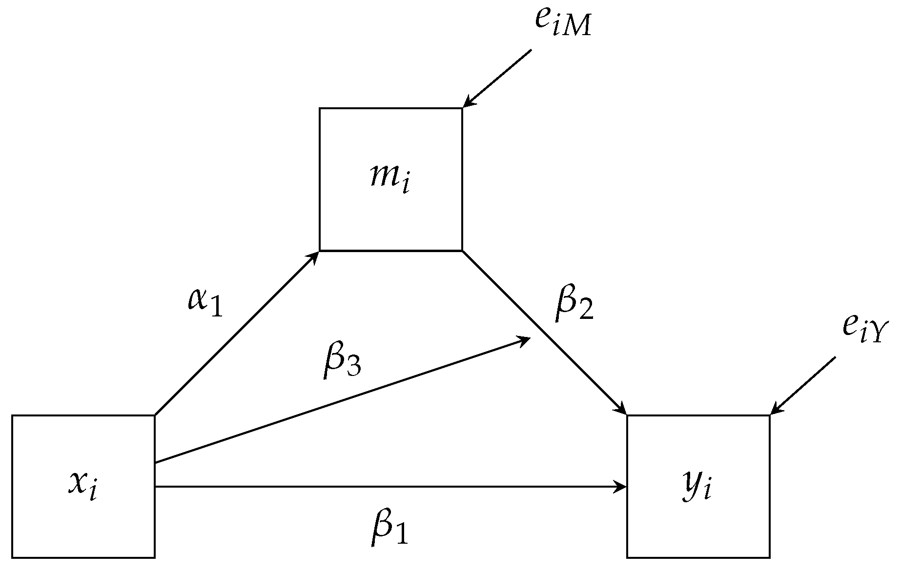
The factored regression framework easily accommodates a wide arrange of path models with incomplete data and nonlinearities. Returning to our moderated regression, suppose we are interested in estimating a meditational process, where M is now a mediator between X and Y. To illustrate, let our analysis consist of a single-mediator interaction model [16].

$$\begin{array}{cc}\hfill y_i& ={\beta }_0+{\beta }_1{x}_i+{\beta }_2{m}_i+{\beta }_3{x}_i{m}_i+e_{iY}\hfill \\ \hfill m_i& ={\alpha }_0+{\alpha }_1{x}_i+e_{iM}\hfill \end{array}$$

(14)

Thus, the mediated effect, $X\to M\to Y$, is given by the product ${\alpha }_1{\beta }_2$ and differs as a function of X (i.e., ${\beta }_3$ coefficient). Figure 1 presents the path diagram for this model. As a convention, we use a path (→) pointing to another path as a representation of a moderated effect. For example, the coefficient ${\beta }_3$ is represented by the path from X to the $M\to Y$ path.

The path diagram has one exogenous variable, X, for which we have not specified a model. As discussed previously, if either X or M are incomplete, a traditional linear SEM software package would require us to improperly estimate the model by assuming a multivariate normal distribution for the product of X and M. The factor regression framework avoids this by explicitly factoring the joint distribution of X, Y, and M as follows.

$$f(X,Y,M)=f(Y\mid X,M)\times f(M\mid X)\times f\left(X\right)$$

(15)

The factorization above differs from Equation (5) by factoring M before X. While the previous moderation model does not preclude us from factoring the model this way, this mediation model requires us to factor the distributions in this order because the $f(M\mid X)$ relationship is of substantive interest. In other words, the factor regression framework directly maps onto how we conceptualize the path model and analysis models. Similar to the moderated regression, when we specify the form of the functional notation, the nonlinear relationship between X and M (i.e., $X\times M$ interaction) will be directly modeled in the conditional distribution $f(Y\mid X,M)$.

The form of the marginal density of X, $f\left(X\right)$, is often specified to be normally distributed with a mean and variance (as is the default in Blimp). However, the general functional notation does not require us to use a normally distributed model. For example, often the X variable in a mediation model is a binary grouping variable. We can easily model a binary variable via a probit regression [23,28,29] model. The probit regression model represents the discrete responses via an underlying normally distributed latent variable with thresholds dividing the latent propensity into observed responses. To illustrate, imagine that X is a binary predictor. We will denote the latent response variable as $X^{\star }$. The link between X and $X^{\star }$ is as follows.

$$\begin{array}{cc}\hfill x_i^{\star }& \sim \mathcal{N}\left(0,1\right)\hfill \\ \hfill x_i& =\left\{\begin{array}{cc}1\hfill & \mathrm{if}{x}_i^{\star }>\tau \hfill \\ 0\hfill & \mathrm{otherwise}\hfill \end{array}\right.\hfill \end{array}$$

(16)

As far as estimation is concerned, the latent response itself is a missing variable, and data augmentation is used to impute the unobserved response per the factorization in Equation (15). Finally, while we illustrate using a probit model to model the binary response, the factored regression specification does allow the use of a logistic model for $f\left(X\right)$. As of Blimp 3.0 [11], a binary logistic model can be estimated using the Pólya-Gamma specification [30,31].

Mediated Latent Variable Model as Factored Regressions

In addition to specifying path models, the factored regression framework can incorporate latent variables and other measurement models. To better explicate this idea, let us modify the mediation model in Equation (14) to allow the mediator to be a latent endogenous variable, $\eta$.

$$\begin{array}{cc}\hfill y_i& ={\beta }_0+{\beta }_1{x}_i+{\beta }_2{\eta }_i+{\beta }_3{x}_i{\eta }_i+e_{iY}\hfill \\ \hfill {\eta }_i& ={\alpha }_0+{\alpha }_1{x}_i+e_{i\eta }\hfill \end{array}$$

(17)

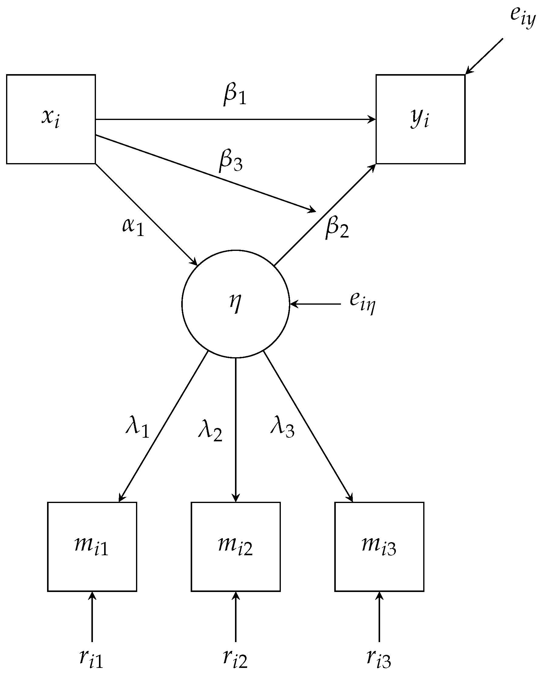
Besides the structural model above, we must also specify a measurement model for the latent factored $\eta$. To illustrate, let us assume that $\eta$ is identified with three items, $M_1$ to $M_3$. In line with traditional factor analysis, we regress the latent factor onto the items.

$$\begin{array}{cc}\hfill m_{i1}& ={\nu }_1+{\lambda }_1{\eta }_i+r_{i1}\hfill \\ \hfill m_{i2}& ={\nu }_2+{\lambda }_2{\eta }_i+r_{i2}\hfill \\ \hfill m_{i3}& ={\nu }_3+{\lambda }_3{\eta }_i+r_{i3}\hfill \end{array}$$

(18)

In Equation (18), we use a subscripted $\nu$ and $\lambda$ to represent the mean structure and loading for a particular item, respectively. Similarly, the double subscripted r is a normally distributed residual or uniqueness for the particular observation and item combination. Figure 2 is the path diagram for both the structural and measurement model, and we exclude the mean structure for simplicity. As a reminder, we use a path pointing to another path as a representation of a moderated effect (i.e., the interaction between the latent $\eta$ and manifest X in Equation 17). The interaction between a latent variable and a manifest variable is an essential feature of our example. As discussed, a traditional linear SEM software assumes multivariate normality among all variables; however, the interaction in our example does not follow this strict multivariate normality and requires specialized methods to estimate [32].

To specify the model via factored regression, we explicitly express the joint distribution of our three indicators ($M_1$ to $M_3$), exogenous predictor (X), and endogenous outcomes ($\eta$ and Y). We then proceed to fully factor this complex joint distribution into a product of conditional distributions.

$$\begin{array}{cc}\hfill f(Y,M_1,M_2,M_3,\eta ,X)& =f(Y\mid M_1,M_2,M_3,\eta ,X)\times f(M_1\mid M_2,M_3,\eta ,X)\times \hfill \\ & \phantom{=m}f(M_2\mid M_3,\eta ,X)\times f(M_3\mid \eta ,X)\times \hfill \\ & \phantom{=m}f(\eta \mid X)\times f\left(X\right)\hfill \end{array}$$

(19)

With the joint distribution fully factored in Equation (19), we then further reduced each conditional model based on the structure we have imposed. More specifically, we can simplify the three conditional distributions associated with the items based upon the imposed factor structure. In other words, our measurement model states that the items are conditionally independent of all other variables given the latent factor. Similarly, the conditional distribution of Y can be simplified as well. With these simplifications, the functional notation for our factored distribution is as follows.

$$\begin{array}{cc}\hfill f(Y,M_1,M_2,M_3,\eta ,X)& =f(Y\mid \eta ,X)\times f(M_1\mid \eta )\times f(M_2\mid \eta )\times \hfill \\ & \phantom{=m}f(M_3\mid \eta )\times f(\eta \mid X)\times f\left(X\right)\hfill \end{array}$$

(20)

Notably, each conditional density on the right-hand side of Equation (20) corresponds to a path in the diagram (Figure 2), and the final density, $f\left(X\right)$, corresponds to an intercept only regression equation for X. Like in traditional linear SEM, constraints are needed to estimate the model, and Blimp, by default, will fix the first factor loading to one (${\lambda }_1=1$) and the intercept for the factor model to zero (${\alpha }_0=0$).

We can estimate the latent mediation model using a similar process to what we previously described. One key difference is that we must obtain imputations for all observations on the latent variable itself. Conceptually, we treat the latent variable no different than a missing manifest variable; the only difference is that every observation is unobserved. Therefore, to obtain imputations on the latent factor, we must sample from the conditional distribution of $\eta$ given all variables and parameters (denoted by ellipses below) for every observation.

$$\begin{array}{cc}\hfill f({\eta }_i^{\left(t\right)}\mid \dots )& \propto f(y_i\mid {\eta }_i,x_i,{\theta }_y)\times f({\eta }_i\mid x_i,{\theta }_{\eta })\times f(m_{i1}\mid {\eta }_i,{\varphi }_1)\times \hfill \\ & \phantom{\propto m}f(m_{i2}\mid {\eta }_i,{\varphi }_2)\times f(m_3\mid {\eta }_i,{\varphi }_3)\hfill \\ & \propto \mathcal{N}\left({\beta }_0+{\beta }_1{x}_i+{\beta }_2{\eta }_i+{\beta }_3{x}_i{\eta }_i,{\sigma }_{eY}^2\right)\times \mathcal{N}\left({\alpha }_0+{\alpha }_1{x}_i,{\sigma }_{e\eta }^2\right)\times \hfill \\ & \phantom{\propto m}\mathcal{N}\left({\nu }_1+{\lambda }_1{\eta }_i,{\sigma }_{r1}^2\right)\times \mathcal{N}\left({\nu }_2+{\lambda }_2{\eta }_i,{\sigma }_{r2}^2\right)\times \mathcal{N}\left({\nu }_3+{\lambda }_3{\eta }_i,{\sigma }_{r3}^2\right)\hfill \end{array}$$

(21)

After sampling imputations on $\eta$ from Equation (21), we condition on those (i.e., treating them as known) at a given iteration and estimate the parameters of the measurement and structural models if they were just linear regressions. Furthermore, the above expression illustrates the fact that we are modeling the interaction relationship between X and $\eta$ by directly accounting for Equation (17) via the density $f(y_i\mid {\eta }_i,x_i,{\theta }_y)$.

Although not immediately apparent, the factored regression specification of the model affords quite a range of flexibility for the relationship of the latent variable and Y. For example, nothing particularly precludes $\eta$ from maintaining only linear or interactive effects. Blimp can easily accommodate other nonlinear relationships (e.g., quadratic, cubic, log-linear) that might be of substantive utility. Finally, while we have imposed normal distributions on the items, the generality of the functional notation allows us to model these regressions as categorical variables easily. For example, the three-item equations in (18) could follow a probit or a logistic model, and in the subsequent section, we illustrate estimating a mediation model with ordinal factor items.

4. Fitting Factored Regressions with Blimp

In this section, we discuss fitting factored regressions to a substantive data example in Blimp (version 3.0 [11]). Below, we review how to factor the models and specify these factorizations with Blimp’s syntax. We include snippets of appropriate syntax and output from running the models to help familiarize readers with estimating and interpreting the results. In addition, we include the complete commented inputs, output, and data set in the supplemental material. Overall, we will look at three analysis examples: (1) a single mediator model, (2) a mediator model with a moderator model, and (3) a latent mediator with a moderator model.

The three analysis examples use a data set that includes psychological correlates of pain severity for a sample of $N=275$ individuals suffering from chronic pain. The main variables for the examples are a biological sex dummy code (0 = female, 1 = male), a binary severe pain indicator (0 = no, minor, or moderate pain, 1 = severe pain), a multi-item depression composite, and a multi-item scale measuring psychosocial disability (a construct capturing pain’s impact on emotional behaviors such as psychological autonomy, communication, and emotional stability), and we provide the variable definitions and missing data rates for these variables in

Table 1. Chronic pain data variable definitions for variables of interest.

Name	Definition	Missing %	Range
male	Biological Sex Dummy Code	0.0	0 or 1
severity	Severe pain dummy code	7.3	0 or 1
depress	Depression composite score	13.5	7 to 28
disability	Psychosocial disability composite	9.1	10 to 34
dep1	Couldn’t experience any positive feelings at all	4.7	1 to 4
dep2	Difficult to work up the initiative to do things	2.2	1 to 4
dep3	I felt that I had nothing to look forward to	1.8	1 to 4
dep4	I felt down-hearted and blue	1.5	1 to 4
dep5	Unable to become enthusiastic about anything	2.2	1 to 4
dep6	I felt I wasn’t worth much as a person	4.0	1 to 4
dep7	I felt that life was meaningless	2.9	1 to 4
disab1	I isolate myself as much as I can from the family	3.3	1 to 6
disab2	I am doing fewer social activities	4.7	1 to 6
disab3	I sometimes behave as if I were confused	3.6	1 to 6
disab4	I laugh or cry suddenly	3.6	1 to 6
disab5	I act irritable and impatient with myself	4.7	1 to 6
disab6	I do not speak clearly when I am under stress	3.6	1 to 6

. The depression scale is the sum of seven 4-point rating scales, and the disability composite is the sum of six 6-point questionnaire items. The first two examples use the continuous sum scores, and the third example uses the item responses as indicators of a latent factor. The examples also include continuous measures of anxiety, stress, and perceived control over pain as auxiliary variables.

Before fitting the models, we will discuss the syntax for reading data into Blimp. The first ten lines of the Blimp script are below, which includes specifying four commands (denoted as capitalized names followed by a colon).

# Read in and set up data

DATA: pain.dat;          # Read Data in

VARIABLES:             # List Variable Names

    id txgrp male age edugroup workhrs

    exercise pain severity anxiety stress

    control depress interfere disability

    dep1:dep7 interf1:interf6 disab1:disab6;

 

ORDINAL: severity male;  # Specify ordinal data

MISSING: 999;        # Missing data code

First, note that Blimp uses a “#” for single-line comments. Second, a semicolon (;) terminates a statement. The DATA command specifies the file path to the data set are reading in. This data set can be tab, space, or comma-delimited. In the above example, we have the pain.dat file in the same folder as the input script, so we do not need to specify the full file path. Next, the VARIABLES command specifies the names and order of the variables in the data set. Blimp also allows these names to appear in the first row of the data set, but then the VARIABLES command must not be used. As a shortcut, Blimp allows specifying multiple variables using a colon. For example, dep1:dep7 is replaced by “dep1 dep2 dep3 dep4 dep5 dep6 dep7”. The ORDINAL command above specifies that the variable severity and male are both ordinal and that we want to model them via a probit specification. Blimp will automatically use the data to determine the number of categories and fit the appropriate ordered probit model. The MISSING command specifies the numerical value that represents a missing value in the data set.

4.1. Fitting a Single Mediator Model

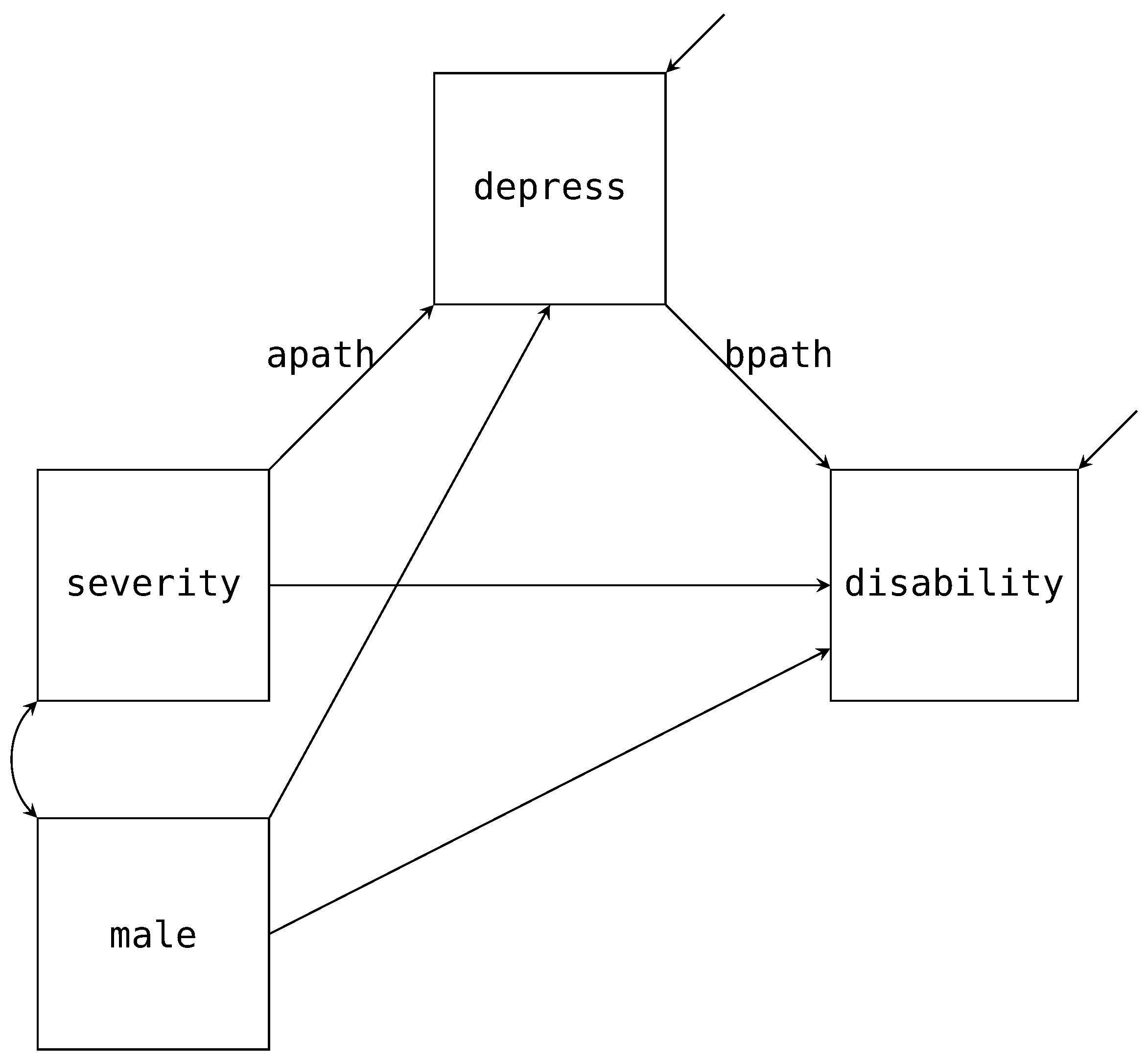
First, we will estimate is a single mediator model that investigates if depression (depress) mediates the effect between pain severity (severity) and the psychosocial disability construct (disability) while controlling for biological sex (male). We provide the path diagram for the model of interest in Figure 3 with the mean structure excluded. To construct the factor regression, we first factor the joint distribution for disability and depress conditional on severity and male.

$$\begin{array}{cc}& f(\mathtt{disability}\mid \mathtt{depress},\mathtt{severity},\mathtt{male})\times \hfill \\ & f(\mathtt{depress}\mid \mathtt{severity},\mathtt{male})\times \hfill \\ & f(\mathtt{severity}\mid \mathtt{male})\hfill \end{array}$$

As already discussed, the factorization maps directly onto the path diagram. For example, Figure 3 has three paths pointing towards depress. These three paths match the same three variables that appear right of the pipe (i.e., ∣). Similarly, we have two paths pointing to depress and the same two variables that appear right of the pipe above. These conditional distributions correspond to the two regression equations we expect from a mediation analysis, and we specify the models via the following Blimp syntax.

# Specify the single mediator model

MODEL:

    # Single-Mediator model controlling for biological sex

    disability ∼ depress@bpath  severity male;

    depress    ∼ severity@apath male;

 

FIXED: male; # Specify no distribution for male

PARAMETERS:  # Post compute the mediated effect

    indirect = apath * bpath;

The MODEL command signifies that we would like to specify our factored models. We list the first factorization, disability conditional on depress, severity, and male, on the first line. A tilde (∼) replaces the pipe in the factorization to specify the appropriate regression model. The @ syntax denotes that we want the regression slope between disability and depress to be labeled as the bpath. The second line after the MODEL command specifies the second factorization, depress conditional on severity, and male and has the apath label. Both of these labeled paths are indicated in Figure 3. Note, we did not specify any regressions for male or severity. By default, Blimp will specify a partially factored model for all predictors (i.e., who are never left of a tilde). Since male is complete, there is no need to include any distributional assumptions about it, and we can indicate this using the FIXED command. Thus, Blimp will by default will estimate the regression of severity on male for us. Alternatively, we could explicitly specify this model by including “severity ∼ male” in the MODEL command.

Finally, the PARAMETERS command allows us to specify quantities of interest. As we will see below, one of the advantages of using simulation methods to estimate the models is that we can easily take the sampled values and create quantities of interest. These quantities will have all the same summarizes as any other parameter (e.g., point estimate, uncertainty, and interval estimates). In this example, we are calculating the mediated effect, saved as the parameter called indirect, by multiplying the apath times the bpath.

In addition to the model syntax, we must specify various settings for the Markov chain Monte Carlo (MCMC) sampler that estimates the model. Below are the four main commands that need to be specified.

# Specify the MCMC sampler parameters

SEED:       398721;  # Set a prng seed

BURN:       1000;  # Set number of burn iterations

ITERATIONS:  10000;  # Set number of post-burn iterations

CHAINS:      4;  # Specify number independent of chains

First, the SEED command is an arbitrary positive integer used to replicate the results of the pseudo-random number generator. While many programs will have a default value if not specified, Blimp purposely requires one to be specified to ensure replicability. Second, the BURN command specifies the number of warm-up iterations the MCMC sampler runs. These iterations will be discarded and not summarized for the parameter summaries. We use the burn-in iterations to ensure convergence, that is, properly sampling from the posterior distributions for the parameters and imputations. We will discuss this more when we look at the output below. Thirdly, the ITERATIONS command requests the total number of post-burn iterations we want to be drawn and summarized as part of the MCMC estimation procedure. Fourthly, the CHAINS command specifies how many independent MCMC processes we want to run. In our example, we are requesting four to be run simultaneously with random starting values. Each chain will be run on a separate processor, allowing us better to utilize the computational power of a modern computer.

4.1.1. Adding Auxiliary Variables to the Model

To supplement the analysis model of interest (Figure 3), we include additional auxiliary variables that will improve estimation with missing data. By adding these additional variables, we hope to better satisfy the missing data assumption about the incomplete observations [33]. Therefore, we also include three continuous measures as auxiliary variables: anxiety (anxiety), stress (stress), and perceived control over pain (control).

To include anxiety, stress, and control into the model as auxiliary variables, we must not substantively change the meaning of the analysis model. We accomplish this by modeling the joint distribution of the auxiliary variables conditional on the predictors and outcomes. Just as we factored the analysis model, we take the joint distribution of the auxiliary variables conditional on the four variables from the analysis (two predictors and two outcomes) and factorize it into the following three conditional distributions.

$$\begin{array}{cc}\hfill & f(\mathtt{anxiety}\mid \mathtt{stress},\mathtt{control},\mathtt{disability},\mathtt{depress},\mathtt{severity},\mathtt{male})\times \hfill \\ \hfill & f(\mathtt{stress}\mid \mathtt{control},\mathtt{disability},\mathtt{depress},\mathtt{severity},\mathtt{male})\times \hfill \\ \hfill & f(\mathtt{control}\mid \mathtt{disability},\mathtt{depress},\mathtt{severity},\mathtt{male})\hfill \end{array}$$

Notably, we include the above factorization is in addition to the factorization that we have already specified for the analysis model. To specify this in Blimp, we replace the previous MODEL command with the following one that includes the factored auxiliary variables.

# Specify the single mediator model

MODEL:

    # Single-Mediator model controlling for biological sex

    disability ∼ depress@bpath  severity male;

    depress    ∼ severity@apath male;

 

    # Model for the Auxiliary Variables

    anxiety ∼ stress control disability depress severity male;

    stress  ∼        control disability depress severity male;

    control ∼                disability depress severity male;

The first two regressions in the syntax are the analysis model that we previously specified. The last three regressions are the three auxiliary models that we will use to better satisfy the missing data assumptions.

By including the auxiliary variables as outcomes regressed on the other variables in our model (i.e., disability, depress, and severity), we explicitly include the conditional distributions into the factorization without changing the meaning of our original analysis model’s densities. In other words, when we draw imputations on the missing variables, these factored regression densities will be a part of the sampling step. To illustrate, the distribution of depress conditional on all other variables is proportional to the product of five densities.

$$\begin{array}{cc}\hfill & f(\mathtt{disability}\mid \mathtt{depress},\mathtt{severity},\mathtt{male})\times f(\mathtt{depress}\mid \mathtt{severity},\mathtt{male})\times \hfill \\ \hfill & f(\mathtt{anxiety}\mid \mathtt{stress},\mathtt{control},\mathtt{disability},\mathtt{depress},\mathtt{severity},\mathtt{male})\times \hfill \\ \hfill & f(\mathtt{stress}\mid \mathtt{control},\mathtt{disability},\mathtt{depress},\mathtt{severity},\mathtt{male})\times \hfill \\ \hfill & f(\mathtt{control}\mid \mathtt{disability},\mathtt{depress},\mathtt{severity},\mathtt{male})\hfill \end{array}$$

Because specifying the auxiliary variable factorization can become tedious as we add more variables, Blimp offers syntax to quickly specify the command in one line.

# Specify auxiliary variable model with one line

anxiety stress control ∼ disability depress severity male;

The above syntax will produce the same exact auxiliary variable models above. In general, we can quickly specify these models by including every auxiliary variable to the left of the tilde and other variables to the right of the tilde.

4.1.2. Output from Single Mediator Model

For the first example, we will give a more broad overview of Blimp’s output, and in the later examples, we will only highlight the essential features that each example introduces. The full output for all models discussed in this article are provided in the supplemental material. Once finished, Blimp’s output opens up with a header giving the software versioning and other information. This header is followed by algorithmic options discussing various aspects of the model, like specified default priors and starting values, and we recommend the interested readers consult the documentation [11] for a discussion of those. The next output section is a table that provides the potential scale reduction factor (PSR or $\widehat{R}$ [25,34]) for the burn-in iterations. The PSR factor represents a ratio of two estimates of the simulation’s posterior variability. As the MCMC algorithm converges to a stationary distribution (i.e., the distribution we are trying to sample from), the two estimates are expected to be equal, resulting in a $\widehat{R}=1.0$.

Blimp calculates the PSR at twenty equally spaced intervals, where we discard the first half of the iterations and use the latter half. Blimp only prints out the highest PSR and the associated parameter number that produced this PSR. A parameter number is given to all estimated, fixed, or generated parameters in the output and, using the command OPTIONS: labels will also print out a table displaying the numbers. As a general rule of thumb, we expect the MCMC sampler to converge once all PSR statistics are below approximately $1.05$ to $1.10$ [25], and the table indicates that the algorithm quickly achieved this within the 1000 burn-in iterations requested.

The next section of the output is more diagnostic information about how well Blimp’s Metropolis sampler performed. As discussed earlier, Blimp uses a Metropolis step within the Gibbs sampler when drawing imputations from the factored distributions. These Metropolis steps require tuning parameters to be controlled so that the imputations are accepted approximately 50% of the time.

Blimp monitors this throughout the process and always prints out one chain’s results by default. If the algorithm fails to tune correctly, an error will be displayed, alerting that more iterations are needed. The above output illustrates that the probability of the sampler accepting imputations for the three missing variables requiring a Metropolis step was approximately 50%.

Following both output sections of diagnostic information, Blimp prints out the sample size and missing data rates of all variables within the model.

In general, this information allows us to double-check that Blimp read the data set correctly, and the output above matches the description of the data in Table 1.

The next output section provides information about the statistical models that we specified. First, Blimp gives the number of parameters across all models. Blimp breaks this into three sections: estimated parameters in the specified models (referred to as an “Outcome Model” in Blimp), generated quantities we specified in the PARAMETERS command, and parameters that are used in the unspecified default models (referred to as a “Predictor Model” in Blimp).

The above output indicates that in total, we have thirty estimated parameters in all specified models and two estimated parameters in the unspecified model for severity. The PREDICTORS section indicates that we have fixed male (i.e., made no distributional assumptions about the complete predictor) and estimated an ordinal probit model for the binary severity variable. The subsequent output then lists all five models that we specified in the syntax and the one generated parameter, indirect.

MODELS

 [1] anxiety ∼ Intercept stress control disability depress severity male

 [2] control ∼ Intercept disability depress severity male

 [3] depress ∼ Intercept severity@apath male

 [4] disability ∼ Intercept depress@bpath severity male

 [5] stress ∼ Intercept control disability depress severity male

 

GENERATED PARAMETERS

 [1] indirect = apath*bpath

By default, Blimp estimates an intercept for all manifest variables, indicated by the special variable name Intercept. This section serves as an overview of the regression equations and reflects the printing order of the models. We can see the three auxiliary models (i.e., regressions for anxiety, control, and stress) and two analysis models with the labeled paths. Finally, there is also a section showing how the generated parameters were computed—i.e., the indirect parameter was computed by multiplying the apath and bpath parameters.

Following the model information, the next section provides the posterior summaries for all specified models.

OUTCOME MODEL ESTIMATES:

 Summaries based on 10,000 iterations using 4 chains.

To reiterate, Blimp defines an “Outcome Model” as any specified relationship in the syntax, including the auxiliary variable models we specified. After the header, Blimp prints the model’s output in the order listed in the Model Information section. For our discussion, we focus on the disability model’s output.

By default, Blimp provides the posterior median, standard deviation, 95% intervals, PSR, and effective sample size (N_EFF). For those unfamiliar with results from a Bayesian analysis, heuristically, we can think of the posterior median and standard deviation as analogous to the point estimate and standard error. Similarly, the 95% posterior interval is comparable to a confidence interval. The PSR is the same PSR we discussed earlier but now computed on all post-burn-in summaries. The effective sample size is a crude approximation of the “effective number of independent simulation draws” ([25] p. 286) for each parameter. Typically speaking, these will be lower than the actual number of samples because of autocorrelation in the MCMC simulation procedure, and it is recommended that more iterations are needed if the effective sample size is less than ten per chain (e.g., less than 40 in our example; [25] p. 287). The model’s output is sectioned into four main categories. The first two sections are the variance parameters and regression coefficients from the model. The next section is the standardized solutions for the regression coefficients. The final section provides the variance explained by the regression coefficients (i.e., $R^2$) and the residual variance. For example, our regression coefficients explained about 20% of the variance, and we are 95% confident the value lies between $0.12$ and $0.29$.

In addition to a summary table for each model’s output, Blimp provides a similar table for the generated indirect quantity.

Just like the proportion of variance explained metrics, this quantity is computed based upon the parameters themselves. Therefore, we obtain posterior summaries, including a 95% posterior interval. The output above illustrates that our indirect effect for the regression of pain severity on disability (i.e., $\mathtt{severity}\to \mathtt{depress}\to \mathtt{disability}$) ranges from $0.43$ to $1.56$ with 95% confidence. The final section of the output is the ancillary model for severity regressed on male. This output also prints out the same posterior summaries but is not of substantive interest. Rather, the model serves to produce imputations for the incomplete predictor, severity.

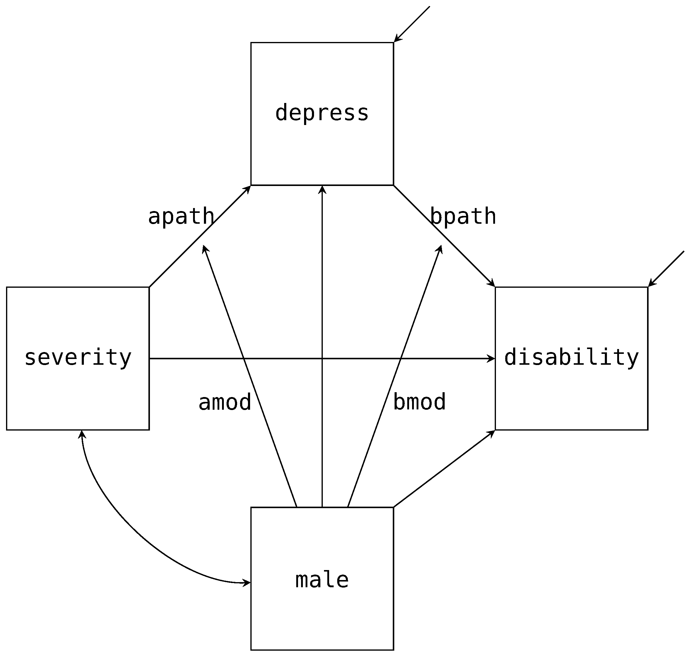
4.2. Single Mediator Model with a Moderator

To continue with our single mediator example, suppose we are interested in investigating if biological sex (male) moderates the A and B paths of the mediation model. The path diagram in Figure 4 adds these two additional paths (labeled amod and bmod in the diagram) with the arrows pointing to the labeled A and B paths. Estimating this model in Blimp is a straightforward extension from the previous example. Notably, the factorization that we discussed in the previous example remains unchanged. What does change is the form of the two substantive models; that is, the models now include the products between male and severity or depress. Below we provide the syntax to extend the mediation model to include the moderated A and B paths.

# Specify the mediation with moderated paths

MODEL:

    # Single-Mediator model with male moderating a and b paths

    disability ∼ depress@bpath  severity male depress*male@bmod;

    depress    ∼ severity@apath male severity*male@amod;

 

    # Specify auxiliary variable model with one line

    anxiety stress control ∼ disability depress severity male;

 

FIXED: male; # Specify no distribution for male

PARAMETERS:  # Post compute the mediated effect

    indirect.female = (apath + (amod * 0)) * (bpath + (bmod * 0));

    indirect.male   = (apath + (amod * 1)) * (bpath + (bmod * 1));

    indirect.diff   = indirect.female - indirect.male;

The above code builds on the previous script. First, we have included the male by depress interaction into the regression and labeled the parameter bmod. Similarly, we have included the male by severity interaction and labeled the parameter amod. Importantly, with these two products added to our regression models, the missing observations in both depress and severity will now be imputed by taking into account the hypothesized nonlinear relationship. Said differently, the likelihoods in the factorizations will directly include the interaction when drawing imputations for missing observations. We have opted to label each moderated path to compute the indirect effects for both males and females. Just like the previous example, we use the PARAMETERS command to post compute the quantities after the sampler estimates the model. The first two lines of the PARAMETERS command computes the indirect effect for females and males, respectively. The third line illustrates that in Blimp, we can use these computed values to calculate the difference in indirect effects between the two groups.

In addition to manually computing the mediated effect for both males and females, Blimp can also produce the conditional regression equations (sometimes referred to as simple effects) for both interactions via the following syntax.

# Specify Simple command to obtain

#   conditional regressions

SIMPLE:

    severity | male;

    depress  | male;

CENTER: severity depress; # Center variables

The SIMPLE command (shown above) can be added on to the script to compute the conditional effect of severity or depress given male equals zero (i.e., females) and one (i.e., males). The variable to the left of the vertical bar is the focal variable, and to the right is the moderator. In our example, because we have specified male as ordinal, Blimp will produce the conditional intercept and slope for each value of the variable. Finally, in line with a typical interaction analysis, we have centered both severity and depress using the CENTER command. Note, by using the CENTER command, Blimp uses the Bayesian estimated mean to center for both variables. This approach allows us to fully capture the mean estimates’ uncertainty and is especially important when the variables are incomplete.

Single Mediator Model with a Moderator Output

Upon running the script, much of the output will be similar to the previously discussed output. This section highlights some of the main differences, and we provide the entire output in the supplemental material. From the model information, the output now displays that we have centered both severity and depress when being used as a predictor.

CENTERED PREDICTORS

 Grand Mean Centered: severity depress

 

MODELS

 [1] anxiety ∼ Intercept stress control disability depress severity male

 [2] control ∼ Intercept disability depress severity male

 [3] depress ∼ Intercept severity@apath male severity*male@amod

 [4] disability ∼ Intercept depress@bpath severity male depress*male@bmod

 [5] stress ∼ Intercept control disability depress severity male

 

GENERATED PARAMETERS

 [1] indirect.female = (apath+(amod*0))*(bpath+(bmod*0))

 [2] indirect.male = (apath+(amod*1))*(bpath+(bmod*1))

 [3] indirect.diff = indirect.female-indirect.male

Note, the centering only occurs when one of the variables is a regressor in a model, and Blimp uses the model parameter for the variable’s mean. In addition to centering, we have the new parameter labels from our analysis models and the generated parameters for the mediated effect for males, females, and the difference between the two groups.

Turning to the output for the disability model again, we present a truncated output table with the standardized coefficients section removed (i.e., where the vertical ellipsis are).

As discussed, we can see that both depress and severity are centered at their overall means for this model; thus, substantively speaking, the interpretation of the intercept is an adjusted mean for the female’s group. In addition, we now have the depress by male interaction, which resulted in an approximately incremental 2% gain in variance explained when compared to the previous model.

Following the disability model, Blimp prints an additional table that provides the conditional effects that we requested with the SIMPLE command.

The table consists of two sets of conditional regression equations. The conditional equations for disability predicted by severity only differ in the intercept because there is no male by severity interaction in this regression. The second set of equations, disability predicted by depress, are the intercepts and slopes holding all other predictors constant at zero (i.e., their means). As with all the generated quantities, the conditional slopes also include 95% posterior intervals that give us a sense of the uncertainty around the parameter. Comparing the female and male slopes, we can see that the interval does not include the other posterior median, which would suggest the slope differences are meaningful and most likely not due to sampling variability.

Finally, the requested generated parameters provide us with the indirect effects for females, males, and the difference between the two effects.

These effects include all the same summaries as before, providing point estimates for each indirect effect and 95% posterior intervals. For example, the output above illustrates that the indirect effect for both males and female are most likely not zero; however, the difference between the two groups is still quite uncertain with the wide posterior interval ranging from $-0.93$ to $1.42$.

4.3. Adding Latent Variables to the Mediation Model

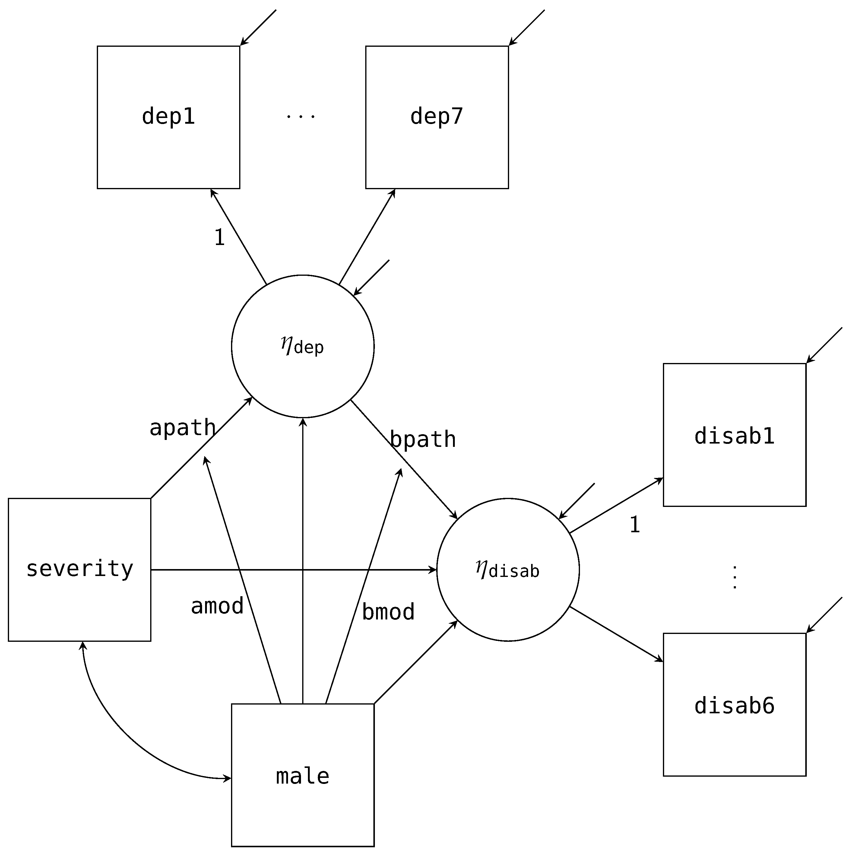
As discussed, factored regression can incorporate measurement models as well. To illustrate the syntax in Blimp, let us look at specifying latent variables for the two multi-item scales: depress and disability. Figure 5 is the path diagram for this model, where the latent factor for depression is normally distributed with seven items as indicators (dep1 to dep7; represented by a set of ellipses in the path diagram), and the latent factor for disability is normally distributed with six items as indicators (disab1 to disab6). As with our previous path diagrams, we have excluded the mean structure from the diagram. In addition, we have fixed the first item for both factors to one for identification.

The structural model’s factorization is similar to that of the single mediator model. The main difference is we are now replacing depress and disability with their latent variables, ${\eta }_{\mathrm{dep}}$ and ${\eta }_{\mathrm{disab}}$. In addition to the structural model, we now must also factor out the measurement model. Multiplying that factorization to the structural model gives us the full functional notation.

$$\begin{array}{cc}& f({\eta }_{\mathrm{disab}}\mid {\eta }_{\mathrm{dep}},\mathtt{severity},\mathtt{male})\times f({\eta }_{\mathrm{dep}}\mid \mathtt{severity},\mathtt{male})\times \hfill \\ & f(\mathtt{disab}\mathtt{1}\mid {\eta }_{\mathrm{disab}})\times f(\mathtt{disab}\mathtt{2}\mid {\eta }_{\mathrm{disab}})\dots \times f(\mathtt{disab}\mathtt{6}\mid {\eta }_{\mathrm{disab}})\times \hfill \\ & f(\mathtt{dep}\mathtt{1}\mid {\eta }_{\mathrm{dep}})\times f(\mathtt{dep}\mathtt{2}\mid {\eta }_{\mathrm{dep}})\dots \times f(\mathtt{dep}\mathtt{7}\mid {\eta }_{\mathrm{dep}})\hfill \end{array}$$

The first line of the factorization above is the structural model, where we are evaluating the mediated effect: $\mathtt{severity}\to {\eta }_{\mathrm{dep}}\to {\eta }_{\mathrm{disab}}$. The second and third lines are the measurement models for the disability and depression factors. Although we have used ellipses instead of writing out the full factored measurement model, all the item models follow the same form. These densities are obtained using the logic we discussed for Equations (19) and (20). Alternatively, we can directly look at the path diagram and deduce that the items are conditionally independent given the latent variables. Finally, because each item is an ordinal variable, we include them in Blimp’s ORDINAL command; therefore, in line with traditional ordinal factor analysis, their regression models will follow an ordered probit specification. Using the factorization that we discussed above, we can specify our model via the following Blimp model syntax.

# Declare latent variables

LATENT: eta_dep eta_disab;

 

# Single-Mediator model with male moderating a and b paths

MODEL:

    # Structural Models

    eta_disab  ∼ eta_dep@bpath  severity male eta_dep*male@bmod;

    eta_dep    ∼ severity@apath male severity*male@amod;

 

    # Measurement Models

    dep1 ∼ eta_dep@1; dep2 ∼ eta_dep; dep3 ∼ eta_dep;

    dep4 ∼ eta_dep;   dep5 ∼ eta_dep; dep6 ∼ eta_dep;

    dep7 ∼ eta_dep;

 

    disab1 ∼ eta_disab@1; disab2 ∼ eta_disab; disab3 ∼ eta_disab;

    disab4 ∼ eta_disab;   disab5 ∼ eta_disab; disab6 ∼ eta_disab;

The LATENT command specifies two new latent variables to add to our data set, eta_dep and eta_disab. By declaring these variables, Blimp will allow us to use them in the MODEL command. As discussed previously, these variables have every observation missing, and each iteration, Blimp will produce imputations via data augmentation according to the model we specified. Mapping onto how we generally conceptualize SEM, we have broken the model syntax down into the structural and measurement parts. The structural part maps onto the same form we specified earlier for the single mediator model. The only difference is replacing the manifest scale scores with their respective latent variables, eta_dep and eta_disab. By default, Blimp excludes the intercept for any latent variable; thus, fixing it to zero for identification. Turning to the measurement model, we specify the regression equations for the two latent variables. In line with standard SEM conventions, we fix the first loading to one (i.e., disab1 and dep1) by using the @ symbol followed by a one. While this syntax matches both the factorization and how Blimp conceptualizes the model, the syntax also allows specifying measurement models concisely using a right-pointing arrow (->).

# Compact syntax to specify measurement models.

eta_dep   -> dep1:dep7;

eta_disab -> disab1:disab6;

The above syntax has two essential features. First, as already mentioned, we use a colon (:) between the names to list all variables names between dep1 to dep7 and disab1 to disab6. Second, when using a right-pointing arrow (->) to predict variables using a factor, by default, Blimp will fix the first variable’s loading to one. Additionally, note that using this syntax still requires the latent variable to be specified via the LATENT command.

Although not shown in Figure 5, we have also included anxiety, stress, and control as auxiliary variables. In line with the previous example, we predict every auxiliary variable as a function of all the other manifest variables in our model. As discussed, this will allow for the imputations on the missing analysis variables to account for the relationship to the auxiliary variables.

MODEL:

    # Specify auxiliary variable model with one line

    anxiety stress control ∼ disab1:disab6 dep1:dep7 severity male;

FIXED: male;         # Specify no distribution for male

PARAMETERS:          # Post compute the mediated effect

    indirect.female = (apath + (amod * 0)) * (bpath + (bmod * 0));

    indirect.male   = (apath + (amod * 1)) * (bpath + (bmod * 1));

    indirect.diff   = indirect.female - indirect.male;

SIMPLE:              # Specify conditional regressions

    severity | male;

    eta_dep  | male;

CENTER: severity;    # Center variables

In addition to specifying the models for the auxiliary variables, we specify that male is fixed with no distribution and post compute the mediated effect for both groups and the difference between the two effects. Finally, we center severity and request for the conditional regression effects for our two focal predictors given the moderator, male.

Latent Single Mediator Model with a Moderator Output

As with the previous example, we highlight some of the main differences in the output and supply the entire output in the supplemental material. The first difference is the number of iterations required for convergence. By including the two latent variables and their ordinal items, the model parameters have gone from a little over thirty to over one hundred free parameters. Therefore, we requested a burn-in of thirty thousand and sampled fifty thousand iterations across four independent chains.

As we can see from the PSR output, our previous burn-in period of one thousand is insufficient to reduce the PSR to acceptable ranges. Increasing the burn-in to thirty thousand adequately reduces the maximum PSR value down well below the 1.05 value suggested by the literature. Therefore, we have reason to believe that the sampler has converged.

Turning to the model printout, we went from five to eighteen conditional models, adding the seven depression and six disability items.

Blimp will list all latent variables first, followed by the manifest variables in alphabetical order. Notably, we see that Blimp conceptualizes an item’s model as the regression of the item onto the latent factor. For example, below is the output for the dep2 regression model.

First, the output has an additional section for the estimated threshold parameters in the ordered probit model. These thresholds break up a normally distributed latent propensity into the observed categories. The loading, $0.747$, is the regression slope for the imputed values of eta_dep, and the standardized coefficient is analogous to the standardized solution in any confirmatory factor analysis. In addition, because there is only one predictor, the proportion of variance explained by the coefficients is equivalent to the estimate of dep2’s reliability under a factor analytic approach. As with other values, Blimp provides the posterior interval for this measure, characterizing the precision in the reliability coefficient.

Moving to the latent disability factor, we provide the output with the standardized coefficients output truncated.

This output illustrates how conceptually nothing has changed compared to using a manifest scale score. The output is no different from any other regression model in Blimp, with estimates of the residual variance, regression coefficients, standardized coefficients (not shown), and the proportion of variance explained. Similarly, the output includes the latent eta_dep by manifest male interaction, and the imputations on eta_dep are drawn in accordance to the nonlinearity. When comparing the above results to the previous example, the scaling of the regression slopes has changed because of the latent variable. Despite this, we can see that we are explaining about 10% more variance with the latent variable ($0.31$ versus $0.21$ with manifest scale score), and this is one of the advantages of incorporating a model to account for the measurement error.

Although we have not presented it, Blimp also produces the conditional regression coefficients and the generated parameters for the latent mediation model. Intrinsically, Blimp does not treat a latent variable differently from a manifest variable. The imputations for either variable are drawn following the factorization discussed throughout the paper and can be saved into multiply imputed data sets.

5. Conclusions

The factored regression framework provides a flexible way to think about complex multivariate modeling problems that arise with missing data. By conceptualizing the problem in terms of the generic functional notation, we can easily focus on specifying the form of each conditional model. In turn, this opens up a wide range of diverse models that are estimable with incomplete data. For example, nothing precludes the factored regression approach from extending to multilevel models. The functional notation itself remains the same. The difference is that the model that represents each function is that of a multilevel model. The free software package we presented, Blimp, can accommodate such multilevel regression models, including the specification of latent variables at all levels. Furthermore, Blimp can accommodate more than just the interaction examples we presented. Blimp will handle any mathematical specification with a wide range of standard math functions at a user’s disposal.

In summary, this article serves as an introduction to the factor regression framework, and we illustrate how to specify the models in Blimp. While we have focused specifically on mediation models, a wide array of examples and syntax are supplied in the Blimp user guide [11].

References

- Ibrahim, J.G. Incomplete data in generalized linear models. J. Am. Stat. Assoc. 1990, 85, 765–769. [Google Scholar] [CrossRef]
- Lipsitz, S.R.; Ibrahim, J.G. A conditional model for incomplete covariates in parametric regression models. Biometrika 1996, 83, 916–922. [Google Scholar] [CrossRef]
- Ibrahim, J.G.; Chen, M.H.; Lipsitz, S.R. Bayesian methods for generalized linear models with covariates missing at random. Can. J. Stat. 2002, 30, 55–78. [Google Scholar] [CrossRef]
- Erler, N.S.; Rizopoulos, D.; Jaddoe, V.W.; Franco, O.H.; Lesaffre, E.M. Bayesian imputation of time-varying covariates in linear mixed models. Stat. Methods Med. Res. 2019, 28, 555–568. [Google Scholar] [CrossRef] [PubMed] [Green Version]
- Erler, N.S.; Rizopoulos, D.; Rosmalen, J.V.; Jaddoe, V.W.; Franco, O.H.; Lesaffre, E.M. Dealing with missing covariates in epidemiologic studies: A comparison between multiple imputation and a full Bayesian approach. Stat. Med. 2016, 35, 2955–2974. [Google Scholar] [CrossRef]
- Zhang, Q.; Wang, L. Moderation analysis with missing data in the predictors. Psychol. Methods 2017, 22, 649. [Google Scholar] [CrossRef]
- Lüdtke, O.; Robitzsch, A.; West, S.G. Regression models involving nonlinear effects with missing data: A sequential modeling approach using Bayesian estimation. Psychol. Methods 2020, 25, 157–181. [Google Scholar] [CrossRef]
- Lüdtke, O.; Robitzsch, A.; West, S.G. Analysis of interactions and nonlinear effects with missing data: A factored regression modeling approach using maximum likelihood estimation. Multivar. Behav. Res. 2020, 55, 361–381. [Google Scholar] [CrossRef] [PubMed]
- Enders, C.K.; Du, H.; Keller, B.T. A model-based imputation procedure for multilevel regression models with random coefficients, interaction effects, and other nonlinear terms. Psychol. Methods 2020, 25, 88–112. [Google Scholar] [CrossRef]
- Rubin, D.B. Inference and missing data. Biometrika 1976, 63, 581–592. [Google Scholar] [CrossRef]
- Keller, B.T.; Enders, C.K. Blimp User’s Guide (Version 3.0); Blimp Software: Los Angeles, CA, USA, 2021. [Google Scholar]
- Robitzsch, A.; Luedtke, O. Model Based Treatment of Missing Data. Available online: https://cran.r-project.org/web/packages/mdmb (accessed on 29 September 2021).
- Bartlett, J.; Keogh, R.; Bonneville, E.F. Multiple Imputation of Covariates by Substantive Model Compatible Fully Conditional Specification. Stata J. 2015, 15, 437–456. [Google Scholar] [CrossRef] [Green Version]
- Erler, N.S.; Rizopoulos, D.; Lesaffre, E.M.E.H. JointAI: Joint Analysis and Imputation of Incomplete Data in R. J. Stat. Softw. 2021, 100, 1–56. [Google Scholar] [CrossRef]
- Gelfand, A.E.; Smith, A.F. Sampling-based approaches to calculating marginal densities. J. Am. Stat. Assoc. 1990, 85, 398–409. [Google Scholar] [CrossRef]
- Judd, C.M.; Kenny, D.A. Process analysis: Estimating mediation in treatment evaluations. Eval. Rev. 1981, 5, 602–619. [Google Scholar] [CrossRef]
- Enders, C.K.; Baraldi, A.N.; Cham, H. Estimating interaction effects with incomplete predictor variables. Psychol. Methods 2014, 19, 39. [Google Scholar] [CrossRef] [PubMed] [Green Version]
- Seaman, S.R.; Bartlett, J.W.; White, I.R. Multiple imputation of missing covariates with non-linear effects and interactions: An evaluation of statistical methods. BMC Med. Res. Methodol. 2012, 12, 46. [Google Scholar] [CrossRef] [Green Version]
- Liu, J.C.; Gelman, A.; Hill, J.; Su, Y.S.; Kropko, J. On the stationary distribution of iterative imputations. Biometrika 2014, 101, 155–173. [Google Scholar] [CrossRef] [Green Version]
- Geman, S.; Geman, D. Stochastic relaxation, Gibbs distributions, and the Bayesian restoration of images. IEEE Trans. Pattern Anal. Mach. Intell. 1984, PAMI-6, 721–741. [Google Scholar] [CrossRef]
- Arnold, B.C.; Castillo, E.; Sarabia, J. Conditional Specification of Statistical Models; Springer Series in Statistics; Springer: New York, NY, USA, 1999. [Google Scholar]
- Arnold, B.C.; Castillo, E.; Sarabia, J.M. Conditionally specified distributions: An introduction. Stat. Sci. 2001, 16, 249–274. [Google Scholar] [CrossRef]
- Albert, J.H.; Chib, S. Bayesian analysis of binary and polychotomous response data. J. Am. Stat. Assoc. 1993, 88, 669–679. [Google Scholar] [CrossRef]
- Kim, S.; Sugar, C.A.; Belin, T.R. Evaluating model-based imputation methods for missing covariates in regression models with interactions. Stat. Med. 2015, 34, 1876–1888. [Google Scholar] [CrossRef] [Green Version]
- Gelman, A.; Stern, H.S.; Carlin, J.B.; Dunson, D.B.; Vehtari, A.; Rubin, D.B. Bayesian Data Analysis; Chapman and Hall/CRC: Boca Raton, FL, USA, 2013. [Google Scholar]
- Lynch, S.M. Introduction to Applied Bayesian Statistics and Estimation for Social Scientists; Springer Science & Business Media: New York, NY, USA, 2007. [Google Scholar]
- Rubin, D.B. Multiple Imputation for Nonresponse in Surveys; Wiley: New York, NY, USA, 1987. [Google Scholar]
- Agresti, A. Analysis of Ordinal Categorical Data, 3rd ed.; Wiley: Hoboken, NJ, USA, 2012. [Google Scholar]
- Johnson, V.E.; Albert, J.H. Ordinal Data Modeling; Springer Science & Business Media: New York, NY, USA, 2006. [Google Scholar]
- Polson, N.G.; Scott, J.G.; Windle, J. Bayesian inference for logistic models using Pólya-Gamma latent variables. J. Am. Stat. Assoc. 2013, 108, 1339–1349. [Google Scholar] [CrossRef] [Green Version]
- Asparouhov, T.; Muthén, B. Expanding the Bayesian Structural Equation, Multilevel and Mixture Models to Logit, Negative-Binomial and Nominal Variables. Struct. Equ. Model. Multidiscip. J. 2021, 28, 622–637. [Google Scholar] [CrossRef]
- Klein, A.; Moosbrugger, H. Maximum likelihood estimation of latent interaction effects with the LMS method. Psychometrika 2000, 65, 457–474. [Google Scholar] [CrossRef]
- Collins, L.M.; Schafer, J.L.; Kam, C.M. A comparison of inclusive and restrictive strategies in modern missing data procedures. Psychol. Methods 2001, 6, 330. [Google Scholar] [CrossRef] [PubMed]
- Gelman, A.; Rubin, D.B. Inference from iterative simulation using multiple sequences. Stat. Sci. 1992, 7, 457–472. [Google Scholar] [CrossRef]
Figure 1.
Path diagram for the single mediator interaction model.
Figure 2.
Path diagram for the single mediator interaction model with latent mediator.
Figure 3.
Path diagram for the single mediator model example.
Figure 4.
Path diagram for the single mediator with moderation example.
Figure 5.
Path diagram for the latent mediation model with moderation example.