Article

Is the Non-Pointness of the Electron Observable in e+e Annihilation at Center-of-Mass Energies 55–207 GeV?

1
School of Physical Sciences, University of Science and Technology of China, No. 96, Jinzhai Road Baohe District, Hefei 230026, China
2
Institute of Physics, Academia Sinica, Taipei 11529, Taiwan
3
Physics and Astronomy Department, Manhattan College, 4513 Manhattan College Parkway, Riverdale, NY 10471, USA
4
Experimental Physics Department, CERN, 1211 Geneva, Switzerland
5
Institute for Particle Physics and Astrophysics, ETH Zurich, Wolfgang-Pauli-Strasse 27, 8093 Zurich, Switzerland
*
Author to whom correspondence should be addressed.
Physics 2023, 5(3), 752-783; https://doi.org/10.3390/physics5030048
Submission received: 15 November 2022 / Revised: 3 June 2023 / Accepted: 10 June 2023 / Published: 10 July 2023
(This article belongs to the Section High Energy Physics)

Abstract

:
The experimental data from VENUS, TOPAS, OPAL, DELPHI, ALEPH and L3 Collaborations collected from 1989 to 2003 are applied to study the quantum electrodynamics (QED) framework through the direct contact interaction term approach, using the annihilation reaction e + e γ γ ( γ ) . The analysis involves performing a χ 2 -test to detect the presence of an excited electron e * , and and evidence of non-point like behavior in the e + e annihilation zone. The analysis yields compelling results, showing a significant signal at a confidence level of approximately 5 standard deviations. These findings suggest the existence of an excited electron with a mass of 308 ± 14 GeV and indicate the presence of a contact interaction characterized by a cutoff scale of 1253.53 ± 226 GeV. Furthermore, the interpretation of the cutoff scale result in terms of a radius of (1.57 ± 0.07) × 10−17 cm raises an intriguing possibility regarding the electron’s non-pointness.

1. Introduction

The electron is one of the most fundamental building blocks of matter, and its discovery over a century ago revolutionized our understanding of the physical world. Since then, it has been the subject of countless investigations, revealing properties that continue to challenge our understanding of nature at the deepest level. A historical account of the electron’s discovery and subsequent study can provide valuable insights into the foundations of modern particle physics.
In 1785, the discovery of Coulomb’s law and in 1820, the discovery of magnetism paved the way for investigating charged particle beams with cathode-ray tubes. By 1869, this possibility was realized.
Charles-Augustin de Coulomb’s law states that the magnitude of the electrostatic force between two point charges is directly proportional to the product of the charges and inversely proportional to the square of the distance between them [1,2].
Three discoveries made in 1820 laid the groundwork for magnetism. Firstly, Hans Christian O ¨ rsted demonstrated that a current-carrying wire produces a circular magnetic field around it [3,4]. Secondly, André-Marie Ampère showed that parallel wires with currents attract each other if the currents flow in the same direction and repel if they flow in opposite directions [5,6,7]. Thirdly, Jean-Baptiste Biot and Félix Savart determined experimentally the forces that a current-carrying, long, straight wire exerts on a small magnet. They found that the forces were inversely proportional to the perpendicular distance from the wire to the magnet [8].
Cathode rays, also known as electron beams or e-beams, are streams of electrons observed in discharge tubes. They are produced by applying a voltage across two electrodes in an evacuated glass tube, causing electrons to be emitted from the cathode (the negative electrode). The phenomenon was first observed in 1869 by Julius Plücker and Johann Wilhelm Hittorf [9,10] and later named “cathode rays” (Kathodenstrahlen) [10,11] by Eugen Goldstein in 1876. In 1897, Joseph John Thomson discovered that cathode rays were composed of negatively charged particles, later named electrons. Cathode-ray tubes (CRTs) use a focused beam of electrons deflected by electric or magnetic fields to create images on a screen [12].
Sir Joseph John Thomson is credited with the discovery of the electron in 1897, the first subatomic particle discovered. He showed that cathode rays were composed of previously unknown negatively charged particles, which must have bodies much smaller than atoms and a very large charge-to-mass ratio [13,14]. Finally, Robert A. Millikan and Harvey Fletcher measured in 1909 the mass and charge separately in the oil drop experiment [15,16,17].
After the discovery of the electron, Max Abraham [18] and Hendric Lorentz [19,20] in 1903 proposed the first models of the electron as an extended spherical electrical charged object with its total energy concentrated in the electric field. However, these models were based on the assumption of a homogeneous distribution of charge density. Although the model provided a means of explaining the electromagnetic origin of the electron’s mass, it also raised the problem of preventing the electron from flying apart under the influence of Coulomb repulsion. Abraham proposed a solution to this inconsistency by suggesting that non-electromagnetic forces (such as, for example, Henri Poincaré stress) were necessary to prevent the electron from exploding. One may say that at that time, modeling the electron within the framework of electromagnetism was deemed impossible. Later, Paul Dirac [21] proposed a point-like model of the electron and recognized the appealing aspect of the Lorentz model [19] regarding the electromagnetic origin of the electron’s mass. Nonetheless, at that time, this idea was found to be inconsistent with the existence of the neutron. Dirac highlighted [21] that although the electron can be treated as a point charge to avoid difficulties with infinite Coulomb energy in equations, its finite size reappears in a new sense in the physical interpretation. Specifically, the interior of the electron can be viewed as a region of space through which signals can be transmitted faster than light.
Arthur Compton firstly introduced the idea of electron spin in 1921. In a paper on investigations into ferromagnetic substances with X-rays [22,23], he writes: “Perhaps the most natural, and certainly the most generally accepted view of the nature of the elementary magnet, is that the revolution of electrons in orbits within the atom give to the atom as a whole the properties of a tiny permanent magnet”. The electron’s spin magnetic moment, μ s , is related to electron’s spin amgular momentum, S, through μ s = g s μ B S / , where the spin g-factor, g s 2 , μ B is the Bohr magneton, and is the reduced Planck constant. The Stern–Gerlach experiment, first proposed by Otto Stern in 1921 and conducted by Walther Gerlach in 1922 [24], inferred the existence of quantized electron spin angular momentum. In the experiment, spatially varying magnetic fields deflected silver atoms with non-zero magnetic moments on their way to a glass slide detector screen, providing evidence for the existence of electron spin. The existence of electron spin can also be inferred theoretically from the spin-statistics theorem and the Pauli exclusion principle. Conversely, given the electron’s spin, one can derive the Pauli exclusion principle [24,25].
The existence of quantized particle spin allows for the possibility of investigating spin-dependent interactions by scattering polarized particle beams on different targets. In nuclear physics, scattering experiments use polarized beam [26,27] sources via electrostatic accelerators such as Tandem accelerators, which can achieve a range of center-of-mass energies from 1.2 MeV [28,29] to 20 MeV [30,31]. There are three types of polarized beams that have been developed: the atomic beam source, which uses the technique of the Stern–Gerlach experiment [32,33], the Lamb-shift source [34,35,36] developed after the discovery of the Lamb shift in 1947 [37], and the crossed-beam source [27,38].
Since 1926, various classical models of spinning point particles have been developed. However, these models face the challenge of constructing a stable point-like particle that includes a single repulsive Coulomb force over a range from zero to infinity.
One model of point-like particles related to electron spin is the Schr o ¨ dinger suggestion [39] that connects electron spin with its Zitterbewegung motion—a trembling motion due to the rapid oscillation of a spinning particle about its classical worldline. The Zitterbewegung concept was motivated by attempts to understand the intrinsic nature of electron spin and involved fundamental studies in quantum mechanics [40,41,42,43,44].
Other types of classical models of point-like spinning particles have been developed. The Yang–Mills model is a class of gauge theories that describe the strong and electroweak interactions in the Standard Model of particle physics. The Weyl model is a spinor field theory that describes massless spin-1/2 particles that do not follow the Dirac equation. The Thirring model is a 1 + 1 dimensional field theory that describes a system of Dirac fermions coupled to a massless bosonic field. It is exactly solvable and has been used as a toy model for studying many-body problems in condensed matter physics. The Gross–Neveu model is a 2 + 1 -dimensional field theory that describes a system of fermions with an interaction term that is quadratic in the fermion field. It is also exactly solvable and has been used to study critical phenomena in condensed matter physics. The Proca model is a relativistic quantum mechanical model that describes a massive vector boson. It is used to describe the massive vector bosons in the electroweak interaction and has been used extensively in the development of the Standard Model. Many reviews and textbooks consider various classical models of point-like spinning particles; some examples include Refs. [45,46,47,48,49]. In general, these kinds of models encounter the problem of divergent self-energy for a point charge and approach this problem in the frame of various generalizations of the classical Lagrangian terms with higher derivatives or extra variables [50,51,52,53,54,55,56,57,58,59] and then restrict undesirable effects by applying geometrical [60,61] or symmetry [62,63] constraints.
The discovery of the Kerr–Newman solution [64] to the Einstein–Maxwell equations in 1965 led to new possibilities for investigating the electron’s structure. Recently, this solution has been used in Ref. [65] to propose a model that considers the interplay between electrodynamics and gravity in the electron’s structure. Coupling electrodynamics with gravity introduces the geometry of De Sitter spaces [66,67], which provides attractive/repulsive forces dependent on distance from the origin and can distinguish between Schwarzschild and De Sitter black holes, ensuring the electron’s stability from the Coulomb repulsion. The theoretical aspects of whether the electron is point-like or not are discussed in Ref. [68].
The modeling of electron structure is driven by the desire to understand fundamental issues, such as the number of fermion families, fermion mass hierarchy and mixing properties, that the Standard Model cannot explain. For example, a natural consequence of the so-called composite models approach [69,70,71,72] to addressing the aforementioned questions is the assumption that quarks and leptons possess substructure. According to this approach, a quark or lepton might be a bound state of three fermions [73] or a fermion and a boson [74]. In many models along this line, quarks and leptons are composed of a scalar and a spin-1/2 preon.Composite models [69,70,71,72] predict a rich spectrum of excited states [69,70,71,72,75] of known particles. Discovering the excited states of quarks and leptons would be the most convincing proof of their substructure. Assuming that ordinary quarks and leptons represent the ground states, it is natural to assign the excited fermions with the same electroweak, color and spin quantum numbers as their low-lying partners. Excited states are transferred to ground states through generalized magnetic-type transitions, where photons (for leptons) or gluons (for quarks) are emitted, as described in Ref. [76]. When excited states have small masses, radiative transition is the main decay mode, but when their masses approach that of the W boson, a large fraction of three-particle final states appear in the decay of excited states.
As discussed above, there is currently no fully predictive model capable of describing the substructure of quarks and leptons. Therefore, one must rely on phenomenological studies of substructure effects, which can manifest in various reactions (see [77] for a review). The search for excited charged and neutral fermions has been ongoing for over 30 years, but to date there has been no success. Quantum electrodynamics (QED) provides an ideal framework for studying potential substructure of leptons. Any deviation from QED’s predictions in differential or total cross-section of e + e scattering can be interpreted as non-point-like behavior of the electron or the presence of new physics. Note that the case of excited quarks [78] is a direct generalization of the lepton case. Theoretical predictions suggest that the transition mechanism of excited quarks, q * , is through gluon, g, emission, q * q g . However, distinguishing this effect from the standard background of three-jet events poses a challenge. As a result, the lepton sector remains the most favorable field for searching for substructure effects from an experimental standpoint. Among the various channels in the e + e scattering experiment, the process of photon pair production e + e γ γ stands out due to its negligible contribution from weak interactions. Additionally, another process of fermion pair production with e + e final state, which is used as the luminosity meter at low angle, is also highly suitable for QED testing in the search for the electron’s substructure. Both processes are presented in Figure 1, left.
The two real photons in the final state of the e + e γ γ reaction are indistinguishable, so the reaction proceeds through the t- and u-channels, while the s-channel is forbidden due to angular momentum conservation. The s-, t-, and u-channels (Mandelstam variables) represent different ways particles interact and exchange energy and momentum. The reaction is highly sensitive to long-range QED interactions, and the two photons in the final state have left-handed and right-handed polarizations which results in total spin of zero, forbidding the s-channel with spin one for γ and Z 0 . As a pure annihilation reaction, the e + and e in the initial state completely annihilate into two photons in the final state, making it easy to subtract the background signal.
The Bhabha reaction e + e e + e is a mixed reaction that occurs via scattering in both the s-channel and t-channel. At energies around the Z 0 pole, the Z 0 contribution dominates. The elastic scattering and annihilation channel are superimposed since the e + and e in the initial and final states are identical. Therefore, the e + e e + e reaction serves as a test for the superimposition of short-range weak interaction and long-range QED interaction.
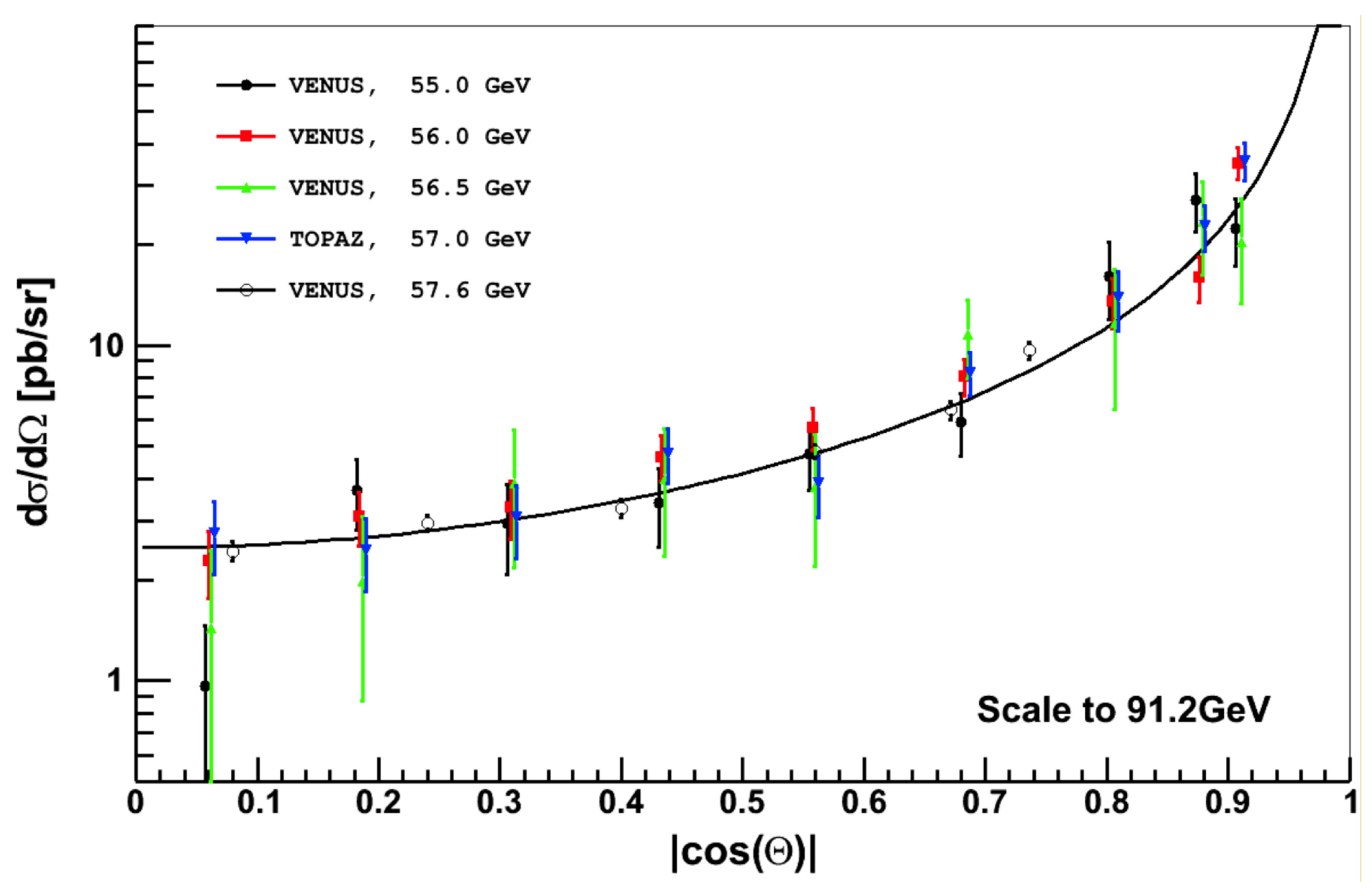
In this paper, we analyze deviations from QED by combining data on the differential cross-section of the e + e γ γ reaction measured via various e + e storage ring experiments. Specifically, the VENUS Collaboration investigated this reaction in 1989 [79] at the center-of-mass energies, s = 55 GeV–57 GeV, while the OPAL Collaboration [80] studied it in 1991 at the Z 0 pole at s = 91 GeV. The TOPAS Collaboration also investigated this reaction in 1992 at s = 57.6 GeV [81], while the ALEPH Collaboration studied it in 1992 at the Z 0 pole at s = 91.0 GeV [82]. Moreover, the DELPHI Collaboration investigated the reaction from 1994 to 2000 at energies ranging from s = 91.0 GeV to 202 GeV [83,84,85], while the L3 Collaboration studied it from 1991 to 1993 at the Z 0 pole, with s = 88.5 GeV to 93.7 GeV [86]. The L3 Collaboration also studied the reaction in 2002 at s ranging from 183 GeV to 207 GeV [87], and the OPAL Collaboration investigated it in 2003 at s ranging from 183 GeV to 207 GeV [88]. Deviations from QED were investigated through the study of contact interactions and excited electron exchange displaced as in Figure 1. Colleagues of some of the authors of this paper have reviewed experimental studies and models of deviations from QED in their Theses [89,90,91]. For earlier review, see [92].
The effective Lagrangian governing a contact interaction exhibits a dependence on the inverse cutoff scale, 1 / Λ , where the power of 1 / Λ is determined by the dimensionality of the fields involved. Additionally, this Lagrangian conserves the helicity of fermion currents. This ensures known particle masses are much less than Λ . Different helicity choices for the fields used in the Lagrangian result in different predictions for angular distributions and polarization observables in reactions where the contact interaction is present. Figure 2b depicts the QED direct contact term, characterized by scale parameters Λ + and Λ , which stand for the cutoff parameter in case of positive and negative interferences, as described in Section 2.5.1. These parameters are subsequently interpreted as being indicative of an extended annihilation radius in the e + e γ γ reaction. Figure 2c depicts Feynman diagrams that are sensitive to the mass of the excited electron, m e * , with the cutoff parameter, Λ e * , being a function of m e * .
In 1989, the VENUS Collaboration [79] established initial limits of Λ + > 81 GeV and Λ > 82 GeV. Table 11 in Ref. [79] provides an overview of other Collaborations that have been studying the same subject. The significance of all analyses was below 1 σ (one standard deviation) and the fitted values of the parameters 1 / Λ 4 and 1 / Λ + 4 were negative. In 2002, the L3 Collaboration [87] established limits on Λ + > 400 GeV, Λ > 300 GeV and m e * > 310 GeV, including negative fit parameters with a significance below 1 σ . In their latest publication on the subject, in 2013 the LEP (Large Electron-Positron collider) Electroweak Working Group [93] conducted an analysis of data from the differential cross-section of all LEP detectors in the energy range of s = 133 GeV to 207 GeV. The group established limits of Λ + > 431 GeV, Λ > 339 GeV and m e * > 366 GeV, which included negative fit parameters with a significance of nearly 2 σ .
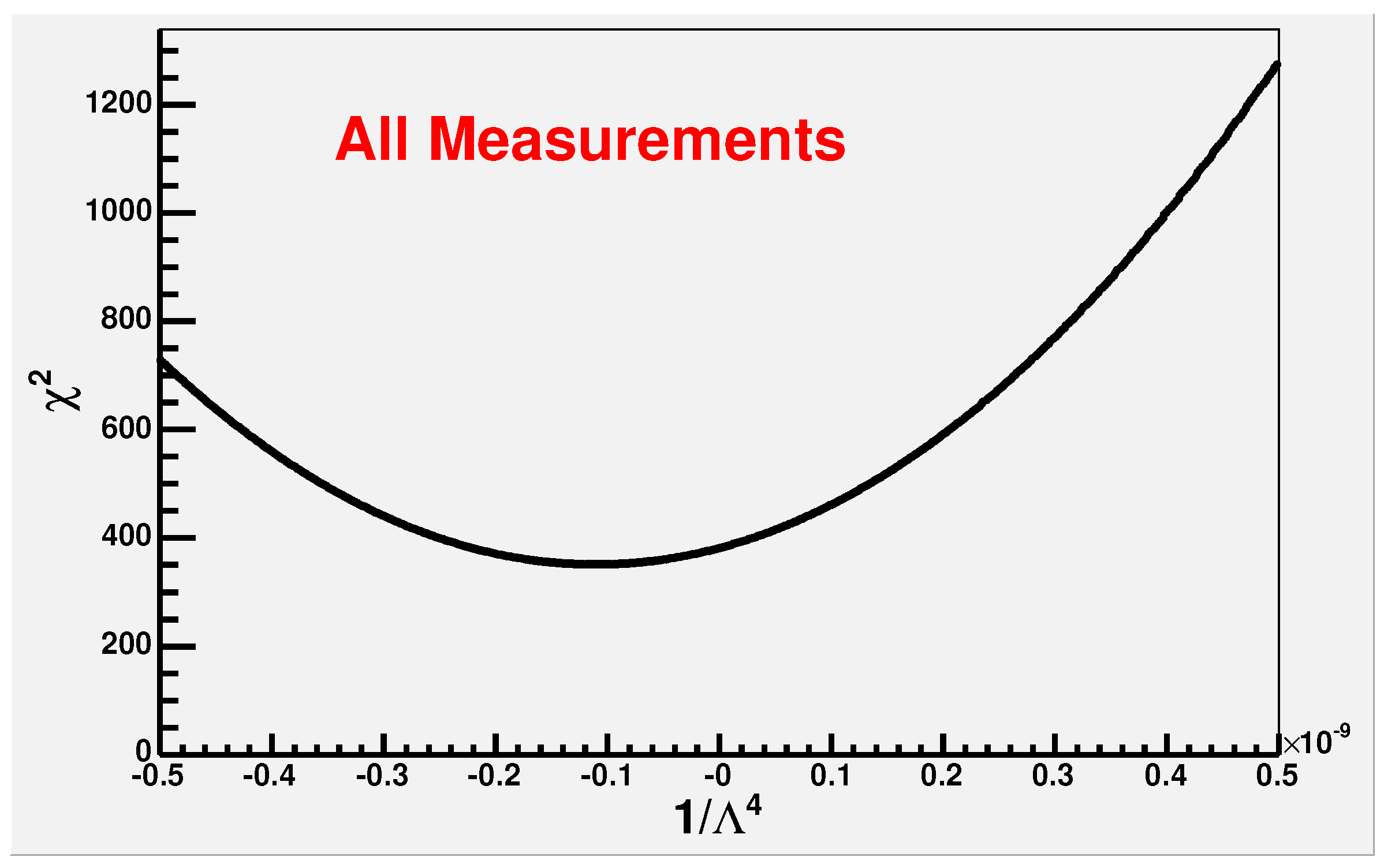
Thus, comparing the results obtained by combining the data from all LEP2 Collaborations with those from L3 alone, it can be observed that the increased statistics have led to more confident results. Based on this observation, we conduct a global fit using data from all six research projects mentioned above to investigate Λ + , Λ , and m e * for s ranging from 55 GeV to 207 GeV, including the corresponding luminosities. An initial attempt to perform the global fit, which involved some of the authors of this paper, has been previously described in detail in Refs. [94,95,96]. It is noteworthy that the global fit revealed a significant deviation of the differential cross-section of the annihilation reaction e + e γ γ from QED predictions, with a statistical significance of 5 σ .
In the current paper, we scrutinize the global fitting procedure by examining all technical details used in the χ 2 -analysis. Section 2 provides a detailed description of the theoretical framework, used for calculating the differential and total cross-sections of the e + e γ γ reaction in QED, including radiative corrections and modifications due to contact interactions and models with excited electrons. Section 3 presents all the data used in the global fitting procedure, along with a description of the cross-section measurement procedure. The χ 2 -analysis, applied for the global fit, is described in Section 4, and in Section 5, we validate the χ 2 -procedure by inferring the total cross-section, which exhibits a similar significance of around 5 σ . The systematic uncertainties of the analysis are discussed in Section 6. In Section 7, we interpret the results of the global fit in the context of the non-pointness of the electron and present conclusions.

2. Theoretical Frameworks

Physical interactions in nature are governed by the principles of local gauge invariance, which are connected to conserved physical quantities of a local region of space. Lagrangian formalism helps to establish the connection between symmetries and conservation laws.
Dirac Lagrangian density describes a free particle of spin 1/2 as follows:
L Dirac = Ψ ¯ ( i γ μ μ m ) Ψ ,
where Ψ is the fermion field, Ψ ¯ = Ψ γ 0 is its adjoint spinor with Ψ the Hermitian congugate of Ψ , γ μ are the Dirac 4 × 4 γ -matrices μ / x μ is the derivative (with x μ being a four-vector with dimensions of length, where μ = 0 denotes time component, and μ = 1 , 2, and 3 the space components), and m is the mass of the particle. The requirement of local gauge invariance leads to the QED Lagrangian,
L QED = Ψ ¯ ( i γ μ μ m ) Ψ + e Ψ ¯ γ μ A μ Ψ 1 4 F μ ν F μ ν ,
where A μ is the gauge field, m A = m γ = 0 , e is the electron charge, e Ψ ¯ γ μ A μ Ψ is the interaction term, and F μ ν = μ A ν ν A μ .

2.1. The Lowest Order Cross-Section of e + e γ γ

The Born-level cross-section [45,97,98,99,100,101] of the e + e γ γ reaction, also known as the leading-order cross-section, is defined by the M -matrix given by
M f i = e Ψ ¯ γ μ Ψ A μ d 4 x ,
where f and i denote the final and initial states, respectively.
At high energies ( s m e 2 ), the mass of the electron can be neglected. Thus, the differential cross-section of the reaction depicted in Figure 2a can be expressed as follows after averaging over the spin states of the initial particles:
d σ 0 d Ω = S 64 π 2 s p f p i M 2 = α 2 s 1 + cos 2 θ k 2 cos 2 θ ,
where Ω cos θ , M 2 is the matrix element, S = 1 / 2 is the statistical factor, the momentum p f = p i , k = E e + / p e + 1 for high energies E e + , where e + denotes the positron, and α = e 2 / 4 π . The angle θ is the photon-scattering angle with respect to the e + e beam axis. The Born-level total cross-section is expressed as
σ 0 = 1 2 α 2 s 0 2 π d ϕ 1 + 1 1 + cos 2 θ k cos 2 θ d ( cos θ ) = 2 π α 2 s ln s m e 2 1 .
As the statistics of the measurements of differential and total cross-sections increases, it becomes essential to account for the radiative corrections discussed below.

2.2. Radiative Corrections

In our analysis, we consider radiative corrections using a Monte Carlo method [97,98,99,100], which incorporates a complete third-order calculation that accounts for electron-mass effects.
The calculations involve six particles: the positron e + with momentum p + , the electron e with momentum p , virtual photons and soft initial photons γ ( k 3 ) with momentum k 3 , as well as hard radiation photons γ ( k 1 ) and γ ( k 2 ) with momentum k 1 and k 2 , respectively. The set of eight virtual photon corrections is illustrated in the Feynman graphs in Figure 3. Figure 4 shows the lowest order Feynman diagrams for two-photon annihilation and the set of corrections, consisting of six soft real photon initial state corrections and eight hard photon corrections [97,98,99,100].
As the exact analytical expression is not available, numerical simulations are used to calculate the corrections of the Feynman diagrams shown in Figure 3 and Figure 4. An event generator [97,98,99,100] was employed to simulate the reaction e + e γ γ ( γ ) . The differential cross-section, including radiative corrections up to O ( α 3 ) , can be expressed as
d σ d Ω α 3 = d σ d Ω Born ( 1 + δ virtual + δ soft + δ hard ) ,
where d σ d Ω Born represents the lowest-order cross-section, while δ virtual , δ soft and δ hard correspond to the virtual, soft-Bremsstrahlung and hard-Bremsstrahlung corrections, respectively.
To differentiate between soft and hard Bremsstrahlung, we introduce a dimensionless discriminator, k 0 1 , into the generator. If the momentum k 3 of the photon from initial state radiation (soft Bremsstrahlung) satisfies k 3 / | p e + | < k 0 , the reaction is considered as two-photon final state; otherwise, it is treated as three-photon final state (hard Bremsstrahlung). To align with the notation used in Equation (4), we use p + as a shorthand for p e + . The two cases are further elaborated on in Section 2.2.1 and Section 2.2.2.

2.2.1. Virtual and Soft Radiative Corrections

If the energies of the photons from initial state radiation (soft Bremsstrahlung) are too small to be detected, i.e., k 3 / | p + | < k 0 , the reaction is treated as a two-photon final state process:
e + ( p + ) + e ( p ) γ ( k 1 ) + γ ( k 2 ) ,
where δ virtual + δ soft are expressed as follows:
δ soft + δ virtual = α π { 2 ( 1 2 v ) ( ln k 0 + v ) + 3 2 1 3 π 2 + 1 2 ( 1 + cos 2 θ ) × [ 4 v 2 ( 3 cos 2 θ ) 8 v cos 2 θ + 4 u v ( 5 + 2 cos θ + cos 2 θ ) + 4 w v ( 5 2 cos θ ) + cos 2 θ u ( 5 6 cos θ + cos 2 θ ) w ( 5 + 6 cos θ + cos 2 ) 2 u 2 ( 5 + 2 cos θ + cos 2 θ ) 2 w 2 ( 5 2 cos θ + cos 2 θ ) ] } ,
where
v = 1 2 ln s m e 2 ,
u = 1 2 ln 2 ( k + cos θ ) m 2 ,
w = 1 2 ln 2 ( k cos θ ) m 2 ,
m = m e p + .
Note that at a low energy regime the expression above includes the mass m e of the electron.
The total cross-section with two γ s in the final state reads
σ 2 γ = σ 0 + 2 α 3 s 2 ( 2 v 1 ) 2 ln k 0 + 4 3 v 3 + 3 v 2 + 2 3 π 2 6 v 1 12 π 2 .

2.2.2. Hard Radiative Corrections

If the energies of the photons from initial state radiation satisfy k 3 / | p + | > k 0 , then the reaction is treated as a three-photon final state process:
e + ( p + ) + e ( p ) γ ( k 1 ) + γ ( k 2 ) + γ ( k 3 ) .
To obtain the differential cross-section of e + e γ γ ( γ ) , one needs to introduce two additional parameters in the phase space. The computation (see [102] for details) is performed in the ultra-relativistic regime, which is as follows:
d σ d Γ i j k = d σ d Ω i d Ω k d x k = α 3 8 π 2 s w i j k F ( i , j , k ) ,
where
w i j k = x i x k y ( z j ) , x i = k i 0 p + ,
y ( z j ) = 2 e x k + x k z j ,
z j = cos ( α i k ) ,
F ( i , j , k ) = P 2 m 2 k j k k 2 k i 2 m 2 k j k k 2 k i + 2 k k k k k j 2 + k j 2 k i k i = P M ( i , j , k )
and α i k is the angle between k i and k j . P binds all permutations of (1, 2, 3). The quantities k i and k i are given by
k i = x i ( k cos θ i )
and
k i = x i ( k + cos θ i ) ,
where θ i is the angle between the momentum of the ith photon and | p + | .
In its turn, the total cross-section with three γ s in the final state reads:
σ 3 γ = 1 3 ! d Γ i j k , i , j , k { 1 , 2 , 3 } ,
where the integral is taken over the phase spaces defined by k 0 < x i < 1 . In practice, Equation (21) can be approximated by an analytical expression, in which the photons are sorted by their energies, such that E γ 1 E γ 2 E γ 3 . Here, γ 1 and γ 2 are treated as annihilation photons, and γ 3 is treated as a hard-Bremsstrahlung photon. Integrating Equation (21) (performed in Refs. [97,98,99,100]), one arrives at
σ 3 γ = 2 α 3 s [ 3 ( ln 4 m 2 1 ) 2 ( 2 ln k 0 + 1 ) ] .

2.3. The Total Cross-Section in e + e γ γ ( γ )

The total cross-section for e + e γ γ ( γ ) is obtained by summing Equations (13) and (22), given by
σ tot = σ 2 γ + σ 3 γ
= σ 0 + 2 α 3 s 4 3 v 3 v 2 + 2 3 π 2 2 v + 2 1 12 π 2 .

2.4. The Numerical Calculation of the e + e γ γ ( γ ) Differential Cross-Section

The third-order differential cross-section is obtained using a Monte Carlo generator [97,98,99,100]. The generator produces events with three photons sorted in descending order of their energies ( E γ 1 E γ 2 E γ 3 ) and at an angle α between photons with energies E γ 1 and E γ 2 , with the correct mixture of soft ( k 3 / | p + | < k 0 ) and hard QED corrections ( k 3 / | p + | > k 0 ), as shown in Figure 3 and Figure 4. The γ -event acceptance range is defined by α min < α < α max . The angle α is analytically related to the scattering angle, θ , thus connecting the limits to | cos θ | .
The binned differential cross-section is calculated as
d σ d Ω i bin = 1 2 π Δ ( | cos θ | ) σ tot N i N ,
where | cos θ | = ( | cos θ 1 | + | cos θ 2 | ) / 2 is the scattering angle, with θ 1 and θ 2 being the scattering angles of photons with energies E γ 1 and E γ 2 , respectively. N i is the number of events in an angular bin width Δ ( | cos θ | ) and N is the total number of generated events.
To search for potential deviations from QED, the generated cross-section (25) is fitted as a function of | cos θ | using a six-parameter χ 2 -fit for each s been analyzed.
As an illustration, we generated one million events at a center-of-mass energy of 189 GeV, within an acceptance range of 14 ° < α < 166 ° , which corresponds to | cos θ | < 0.97 . We used a soft/hard discriminator of k 0 = 0.01 and distributed the events over 50 Δ ( | cos θ | ) bins. The resulting χ 2 -fit of the differential cross-section exhibits the following polynomial behavior
d σ d Ω QED = d σ d Ω Born × 1 + p 1 + p 2 exp x 1.2 2 p 3 2 + p 4 x + p 5 x 2 + p 6 x 3 ,
where x = | cos θ | and
p 1 = 0.2869 , p 2 = 0.51851 , p 3 = 0.19946 , p 4 = 0.39652 , p 5 = 0.41213 , p 6 = 0.70428 .
We note that e + e γ γ ( γ ) channel lacks a comprehensive analysis of theoretical uncertainty, specifically the uncertainty associated with the third-order Monte Carlo prediction. In a QED process, higher-order effects can be approximated to be 10% ( α ) of the correction caused by the highest-order corrections. The theory uncertainty can be estimated to be 10% of the radiative correction for each experiment, with a minimum of 0.5%.

2.5. Deviations from QED

If QED is a fundamental theory, it should be capable of describing the experimental parameters of the e + e γ γ ( γ ) reaction up to the Grand Unification scale. However, currently, QED has only been tested up to center-of-mass energy 100 GeV. Therefore, at higher energy scales, new non-QED phenomena may become observable. If a cutoff scale parameter is found, it can serve as a threshold point for the breakdown of QED and the emergence of new underlying physics. This paper focuses on the mass of the excited electron and the cutoff scale of the contact interaction, which can be interpreted in terms of the size of the electron.

2.5.1. Heavy Electron Mass

This model assumes the existence of an excited state of the electron and the reaction e + e γ γ occurs through the exchange of a virtual excited electron e * in the t- and u-channels, as shown in the Feynman graph in Figure 2c. The interaction is characterized by a coupling between the excited electron and the ordinary electron, as well as between the excited electron and the photon. A magnetic interaction term is introduced [76,103] to account for this interaction in the form,
L e * = e λ 2 m e * Ψ ¯ e * σ μ ν Ψ e F μ ν ,
where λ is the relative magnetic coupling strength to the QED magnetic coupling and σ μ ν = 1 2 γ μ , γ ν . The QED differential cross-section modified by this interaction reads:
d σ d Ω = d σ d Ω QED 1 + s 2 2 λ 2 m e * 4 1 cos 2 θ F ( cos θ ) ,
where F ( cos θ ) is given by
F ( cos θ ) = 1 + s 2 m e * 2 1 cos 2 θ 1 + cos 2 θ × 1 + s 2 m e * 2 2 s 2 m e * 2 2 cos 2 θ 1 .
At condition s / m e 2 2 < < 1 , the expression (29) is reduced to
d σ d Ω = d σ d Ω QED ( 1 ± δ new ) = d σ d Ω QED 1 ± s 2 2 1 Λ ± 4 ( 1 cos 2 θ ) ,
where the scale Λ + = Λ e * is related to m e * by Λ + 2 = m e * 2 / λ and negative contribution Λ is added for symmetry.

2.5.2. Minimal Interaction Length and Non-Pointness of the Electron

The effective Lagrangian for a contact interaction uses current fields of known particles and is proportional to the lowest power of 1 / Λ , which depends on the dimensionality of the fields used. When constructing this Lagrangian, it is important to ensure that fermion currents conserve helicity, which is necessary for composite models. This condition ensures that known particle masses are much less than the energy scale of Λ . Different choices of helicity for the fields used in the Lagrangian result in different predictions for the angular distributions and polarization observables in reactions where the contribution of the contact interaction is considered.
In Refs. [104,105,106,107,108,109,110], the contact interaction between two fermions and two bosons was studied in a general case. In the following discussion, we focus on the simplest dimension-6 operator, which is described by the effective Lagrangian
L 6 = i Ψ ¯ γ μ ( D ν Ψ ) ( g 6 F μ ν + g ˜ 6 F ˜ μ ν ) ,
where coupling constant g n , where n = 6 , is related to the energy scale of Λ by g n = 4 π / Λ ( n 4 ) . The QED covariant derivative is represented by D μ = μ i e A μ with A μ standing for covariant four-potential of the electromagnetic field and the dual of the electromagnetic tensor is F ˜ μ ν , given by F ˜ α β = 1 2 ε α β μ ν F μ ν . The modified differential cross-section reads:
d σ d Ω T = d σ d Ω QED 1 ± δ new = d σ d Ω QED 1 ± s 2 2 α 1 Λ 4 + 1 Λ 4 ˜ ( 1 cos 2 θ ) ,
in the following we use Λ = Λ ˜ = Λ 6 and omit higher-order terms such as Λ 7 or Λ 8 in δ new .
A common method for searching for deviations from QED is to use a χ 2 -test to compare experimentally measured cross-sections with predicted QED cross-sections. To incorporate a non-QED direct contact term into the QED cross-section, an energy scale Λ is introduced via Equation (33). Λ can be interpreted as defining the size of the object where annihilation occurs, which can be calculated using either the generalized uncertainty principle [111,112,113] or the electromagnetic energy, E, and wavelength, λ γ ,114] of the light emitted by the object. The wavelength, λ γ , must be smaller or equal to the size of the interaction area. If the χ 2 -test exhibits a minimum for a certain Λ , the latter defines the region in which e + e annihilation must occur via Λ = E = ν γ , where ν γ = c / λ γ with c the speed of light. We assume that λ γ = r e regulates the size of the electron according to
r e = c / Λ .
Equation (34) provides a generic formula for calculating the size of an object, which can be obtained using the generalized uncertainty principle [115,116,117]. It is worth noting that as Λ approaches infinity in Equation (34), the size of the object tends to zero: r e 0 .

3. The Measurement of the Total and Differential Cross-Section

The e + e γ γ ( γ ) reaction initiates in storage e + e ring accelerators a background-free signal in a detector. For example, Figure 5 shows a typical event display captured in the central detector’s cross-section of the L3 detector at LEP, providing a representation of the signal appearance. Similar signals have been observed in all LEP detectors, as well as in VENUS and TOPAS detectors. The channel’s topology is clean and the event selection is based on the presence of two energetic clusters in the electro-magnetic calorimeter (ECAL). The two highest-energy clusters must meet a minimum energy requirement. The cuts on acollinearity or missing longitudinal momentum, as well as the allowed range in polar angle, of the observed clusters, have been applied. Charged tracks are generally not allowed, except when they can be associated with a photon conversion in one hemisphere, in order to remove background, particularly from Bhabha events.
The limited coverage of the ECAL, along with selection cuts to reject events with charged tracks, reduces the signal efficiency. The impact of the above-mentioned cuts varies significantly depending on the detector geometry, resulting in uncorrelated systematic errors across LEP experiments, VENUS and TOPAS.
The total cross-section is calculated as the ratio of the number N of detected events within the full angular coverage of the ECAL to the efficiency, ε , and the integrated luminosity, L,
σ tot = N ε L .
The binned differential cross-section is calculated as
d σ d Ω i bin = 1 2 π Δ ( | cos θ | ) i · N i L · ϵ i ,
where i defines the angular bin. To compare the measured differential cross-section given in Equation (36) with QED predictions in the ith bin, the average value of cos θ is calculated as
cos θ i = | cos θ | i | cos θ | d σ d Ω ( | cos θ | ) e + e γ γ Born d | cos θ | | cos θ | i d σ d Ω ( | cos θ | ) e + e γ γ Born d | cos θ | .
Here, cos θ is defined as 0.5 ( | cos θ 1 | + | cos θ 2 | ) , where cos θ 1 and cos θ 2 are the scattering angles of the first and second photon, respectively. The average calculation is based on the QED Born-level prediction. The Collaborations present their data in bins of cos θ i where the cross-section is calculated based on the number of events in each bin. Therefore, each value of cos θ i corresponds to the low edge of the bin.

Differential Cross-Section Datasets

This Section describes the data on the differential cross-section of the reaction e + e γ γ that are included in the global fit analysis. The data are reweighted for a single center-of-mass energy, E scale , and presented by plotting the reweighted results along with the QED- α 3 cross-section (6). Since the measurements of the cross-section are obtained with varying event numbers, N i , and at different center-of-mass energies, E i , the reweighting is necessary to enable the visual comparison of different datasets. This is illustrated in Figure 6, Figure 7, Figure 8, Figure 9, Figure 10 and Figure 11.
The reweighting is performed using the equation,
d σ d Ω | cos θ | j scale = i r N i d σ d Ω | cos θ | j i · E i E scale 2 i r N i .
In Equation (38), N i is used to derive the differential cross-section at s = E i , where i = 1 to r, which represents the number of values d σ d Ω i | cos θ | j to be scaled. Here, j is the cos θ bin number and cos θ j is calculated using Equation (37). The plots in Figure 6, Figure 7, Figure 8, Figure 9, Figure 10 and Figure 11 are obtained with E scale = 91.2 GeV. A deviation from QED in the differential cross-section of the e + e γ γ reaction would manifest as an observation of a difference between the QED and experimental differential cross-sections.
The VENUS Collaboration presented the luminosity, e + e γ γ candidates, angular distribution and differential cross-section at four center-of-mass energies s = 55.0 GeV, 56.0 GeV, 56.5 GeV and 57.6 GeV; see Tables 2–4, and 8 in Ref. [79]. The TOPAS Collaboration presented the luminosity and differential cross-section, with bin width, at s = 57.0 GeV; see Tables 1 and 2 in Ref. [81]. Figure 6 displays the reweighted data from the VENUS and TOPAS experiments, obtained using Equation (38) with E scale = 91.2 GeV, with the QED- α 3 differential cross-section at s = 91.2 GeV (black line).
The ALEPH Collaboration provided measurements at s = 91.3 GeV, as well as the bin width; see Table 8.2 in Ref. [82]. Figure 7 shows the ALEPH data scaled to s = 91.2 GeV using Equation (38). Only statistical uncertainties are displayed. The black line corresponds to the QED- α 3 differential cross-section at s = 91.2 GeV.
The DELPHI Collaboration published data in Refs. [83,84,85] from 1994, 1998 and 2000. The year 1994 results in Ref. [83] show the luminosity at s = 91.25 GeV and the differential e + e γ γ cross-section, together with the bin width and number of events per bin. The year 1998 results in Ref. [84] show the same measurements at s = 91.25 GeV, 130.4 GeV, 136.3 GeV, 161.5 GeV 172.4 GeV and 182.7 GeV. The measurements at s = 188.63 GeV, 191.6 GeV, 195.5 GeV, 199.5 GeV and 201.6 GeV are presented in Ref. [85] describing the year 2000 results. Figure 8 displays the DELPHI data scaled with Equation (38) to s = 91.2 GeV. Again, the black line represents the QED- α 3 differential cross-section at s = 91.2 GeV, and only statistical uncertainties are shown.
In Ref. [86], L3 Collaboration published measurements of the differential cross-section, the data on bin size and event counts obtained in 1995 at s = 91.2 GeV. The year 2000 results in Refs. [118,119,120,121] show the same measurements at s = 183 GeV and 189 GeV. The measurements at s = 192 GeV, 196 GeV, 200 GeV, 202 GeV, 205 GeV and 207 GeV are presented in Ref. [87] describing the year 2002 results. Figure 9 displays all L3 differential cross-section data at s = 91 GeV to 207 GeV, scaled with Equation (38) to 91.2 GeV; only statistical uncertainties are shown. As above, the black line represents the QED- α 3 differential cross-section at s = 91.2 GeV.
Figure 9. Same as Figure 6, but with the data by L3 [86,87,118,119,120,121].
Physics 05 00048 g009
Figure 10. Same as Figure 6, but with the data by OPAL [80,88].
Physics 05 00048 g010
In Ref. [80], OPAL Collaboration published measurements of the differential cross-section, the data on bin size and event counts obtained in 1991 at s = 91.0 GeV. The year 2003 results in Ref. [88] show the same measurements at s = 183 GeV, 189 GeV, 192 GeV, 196 GeV, 200 GeV, 202 GeV, 205 GeV and 207 GeV. Figure 10 displays all the OPAL differential cross-section data from s = 91 GeV to 207 GeV, scaled with (38) to 91.2 GeV. Only statistical uncertainties are shown. Again, the black line is the QED- α 3 differential cross-section at s = 91.2 GeV.
Figure 11 combines the differential cross-sections measured by VENUS, TOPAS, ALEPH, L3 and OPAL at the range s = 55 GeV to 207 GeV. All data points are scaled with Equation (38) to 91.2 GeV and only statistical uncertainties are displayed. The black line represents the QED- α 3 differential cross-section at s = 91.2 GeV.
Figure 11. Differential cross-section of the e + e γ γ reaction from VENUS, TOPAS, ALEPH, L3 and OPAL. The black line is the QED- α 3 cross-section (6). The colours and symbols are same as in Figure 6, Figure 7, Figure 8, Figure 9 and Figure 10.
Physics 05 00048 g011
No significant deviations from QED predictions are seen in Figure 6, Figure 7, Figure 8, Figure 9, Figure 10 and Figure 11. In Section 4 just below, we perform a global χ 2 -fit to the combined dataset.

4. Global χ 2 -Test of the Differential Cross-Section

The non-QED model parameters, discussed in Section 2.5, are determined by applying a χ 2 -test to the combined differential cross-section data measured by the VENUS, TOPAS, OPAL, DELPHI, ALEPH and L3 Collaborations. The following expression is minimized using the MINUIT code [122,123] from for the χ 2 -test:
χ 2 = i , j d σ d Ω meas ( | cos θ | i , E j ) d σ d Ω new ( | cos θ | i , E j , Λ ) Δ d σ d Ω meas ( | cos θ | i , E j ) 2 .
Here, d σ d Ω meas ( | cos θ | i , E j ) is the measured differential cross-section at an angular bin (i) and a center-of-mass energy bin (j), while and d σ d Ω new ( | cos θ | i , E j , Λ ) is the QED- α 3 differential cross-section in the same bins and a test parameter Λ , as defined in Equations (31) and (33). The “±” sign in front of δ new in Equations (31) and (33) allows the χ 2 -test to search for positive and negative interference. The term Δ d σ d Ω meas ( | cos θ | i , E j ) is the uncertainty of the mean value of the measurements, which is represented by sum in quadratures of the statistical and systematic uncertainty (to be discussed in Section 6). The χ 2 -test requires details of the differential cross-section and the luminosity at the different center-of-mass energies at which the data were taken. The Section 3 provided a description of the dataset utilized in the analysis, which included individual sub-sets published by the Collaborations. Table 1 provides a summary of the luminosities for all sub-sets from VENUS, TOPAS, ALEPH, DELPHI, L3, and OPAL used in the χ 2 -test.

4.1. Global χ 2 -Test for Heavy Electron m e *

In order to perform the χ 2 -fit in Equation (39), it is necessary to use the differential QED cross-section (26) for a given center-of-mass energy, as well as the differential cross-section calculated for the heavy electron, see Equations (29) and (30). The χ 2 -fit can be performed separately for every data sub-set at respective s by either utilizing the experimentally measured differential cross-section if available, or calculating it using the luminosity, n umber of events per angular bin width and effiiency, as described in Equations (36) and (37). The theoretical QED- α 3 differential cross-section is computed using the numerical calculations of the e + e γ γ ( γ ) reaction discussed in Section 2.4. The parameter 1 / Λ + 4 is used in the cross-section (31) for the test. Table 2 displays the resulting fit parameters ( 1 / Λ + 4 in 1 / GeV 4 ) and fit quality parameter χ 2 / dof (degrees of freedom) of the χ 2 -test for every data sub-set.
About 80% of the data sub-sets in Table 2 exhibit a preference for negative values of 1 / Λ + 4 . This trend is also evident in Figure 12 and Table 3. Figure 12 displays the results of the χ 2 tests for the data sub-sets, grouped according to their Collaborations (ALEPH, DELPHI, L3, OPAL) and combinations of Collaborations such as TRISTAN (TOPAS and VENUS), LEP1 and LEP2. The trend towards negative values of 1 / Λ + 4 becomes more pronounced as the statistics of the grouped combinations increases.
Table 3 shows the values of 1 / Λ 4 , obtained from the fits to the data combined in groups of Collaborations. For TRISTAN, the values are positive with the large error bar for energies ranging from s = 55 GeV to 57.6 GeV. At LEP1, where the data were taken at the Z 0 pole with lower luminosity, the values are already negative with a statistical significance of approximately one standard deviation. This is reflected in the size of the error bars in Table 3. The LEP2 data, covering energies from 133 GeV to 207 GeV, have much higher luminosity and dominate the global fit result. The fitted parameter is negative with a significance of approximately five standard deviations in this energy range. Note that the χ 2 -distribution exhibits a good parabolic shape, as shown in Figure 13. This shape remains almost unaffected when applying the non-parabolic χ 2 in the MINOS routine of the MINUIT program [122,123]. Therefore, the significance deduced from the parabolic shape remains the same.
The best fit value of the parameter 1 / Λ 4 obtained from the χ 2 -fit is shown in Figure 13 and given in Table 4. It has a significance of about five standard deviations, which implies the existence of an excited electron with a mass of m e * = 308 ± 14 GeV, as interpreted through Λ + 2 = m e * 2 / λ , where λ = 1.0 .

4.2. Global χ 2 -Test for a Non-Pointness of the Electron

The ( 1 cos 2 θ ) dependence of the differential cross-section is the same for both the excited electron model (31) and the contact interaction (33). Therefore, the same MINUIT framework can be used to perform the χ 2 test by equating Λ = Λ ˜ = Λ 6 in Equation (39).
The difference between Equation (33) and Equation (31) lies only in the presence of the constant α , but it does not affect the significance of the fit, as shown in Table 4 and Table 5. The result indicates the existence of a contact interaction with a significance of about five standard deviations and a cutoff scale of Λ = 1253.53 ± 226 GeV.
Note that the p-value gives a significance result that is similar to the χ 2 -test, as demonstrated in detail in the total cross-section analysis [124].

5. Indication of a Signal in the Total Cross-Section

It would be instructive to verify whether a signal indicating the existence of the excited electron and contact interaction is also present in the total cross-section of the e + e γ γ ( γ ) reaction.
Studying the sensitivity of the χ 2 test to the total experimental cross-section, σ tot , of the e + e γ γ reaction, represented by combined data from different Collaborations within the energy range 55 GeV to 207 GeV, is a major challenge. This is due to the fact that different experiments measured σ tot at different ranges of the angle θ and with different efficiencies ε at the same or similar center-of-mass energy. On the other hand, the Collaborations compare their measured σ tot with a Monte Carlo-simulated [97,98,99,100] QED total cross-section, σ QED , which is either the same or very similar across all Collaborations. Therefore, we choose to use a benchmark L3 detector and normalize the total cross-sections measured by other detectors with respect to that of L3, along with the corresponding number of events, as described in Ref. [124] in detail. This approach enables us to properly combine the center-of-mass energy points where more than one detector has provided measurements of the total cross-section. Thereby, one can construct ratios, R ( exp ) = σ tot comb / σ QED , by comparing the combined measured total cross-section, σ tot comb , to the simulated one σ QED , at each available center-of-mass energy. The uncertanties for σ tot comb ( Δ σ tot comb ) and R ( exp ) ( Δ R ( exp ) ) are also calculated. The processed numerical values, initially obtained in Ref. [124], are listed in Table 6 and displayed in Figure 14.
No significant disagreement between the combined measured total cross-section, σ tot comb and the predicted value, σ QED , of the e + e γ γ reaction in the center-of-mass energy range 55.0 GeV ≤ s ≤ 207 GeV is observed in Figure 14. The decrease in uncertainties is observed at higher center-of-mass energy bands (LEP energies) due to the contribution of multiple detectors to each s point. To show the potential impact of the parameters inferred at 5 σ significance from the χ 2 -test of the differential cross-section, we plot in Figure 15 the ratio R ( exp ) along with the ratio R ( Λ 6 ) = σ QED , tot L 3 / σ QED + Λ top , tot L 3 , where σ QED , tot L 3 and σ QED + Λ top , tot L 3 are, respectively, the pure QED and the excited electron (contact interaction) modified at Λ = 1253.53 GeV total cross-sections normalized with respect to the L3 detector. For R ( Λ 6 ) , we adopt an analytical approximation,
R ( Λ 6 ) = C 4 C 1 tanh ( C 3 s + C 2 ) ,
where the constants C 1 = 0.0732964 , C 2 = 3.06655 , C 3 = 0.0127994 and C 4 = 0.928311 are obtained from the fit of the Monte Carlo-generated numerical results on R ( Λ 6 ) . The experimental data show (Figure 15) a deviation from the QED prediction above s = 180 GeV.
In sum, Figure 15 indicates a deviation between the total cross-section of the measured data and the QED prediction, in contrast to the differential cross-section test shown in Figure 6, Figure 7, Figure 8, Figure 9, Figure 10 and Figure 11. The data tend to lie below the horizontal line in the energy range s 180 GeV, with R ( Λ 6 ) being approximately 4.0% lower than the QED predicted values.

6. Systematic Uncertainties

Various sources of systematic uncertainties affect the measurement, including uncertainties from the luminosity evaluation, selection efficiency, background estimation, choice of QED- α 3 theoretical cross-section, fit procedure, fit parameter and the choice of scattering angle in | cos θ | for comparison between data and theory. The maximum estimated uncertainties from luminosity, selection efficiency and background evaluations contribute approximately δ Λ / Λ = 0.01 to the total systematic uncertainty in the estimated fit parameter. The choice of theoretical QED cross-section was validated using about 2000 e + e γ γ ( γ ) events generated and processed with the geometry and selection cuts of the L3 detector [97,98,99,100,101]. For scattering angles close to 90 where | cos ( θ ) | experiment 0.05 , the systematic uncertainty contribution ( δ Λ / Λ ) δ | cos θ | is approximately 0.01. The combined effect of these two systematic uncertainties yields the uncertainty of δ Λ / Λ 0.015 . In a small sample of e + e γ γ ( γ ) events, fit values were compared using χ 2 , maximum likelihood, Smirnov–Cramer von Mises and Kolmogorov tests with and without binning [125]. An additional uncertainty of δ Λ / Λ = 0.005 was inferred from the fit procedure variation study. In summary, while multiple sources of systematic uncertainties have been identified, they are all smaller than the statistical uncertainty of the experimental data.
A slight deviation in R ( exp ) from the σ ( QED ) tot cross-section appears in Table 6 and Figure 15 above s = 91.2 GeV. The systematic uncertainty for the measured total cross-section above s > 91.2 GeV ranges from 0.10 pb to 0.13 pb for L3 (see Table 3 in [87]), 0.09 pb to 0.14 pb for DELPHI (see Table 4 in [83]) and 0.05 pb to 0.08 pb for OPAL (see Table 7 in Ref. [87]). The systematic uncertainty for the total QED cross-section of each detector is taken at the level of the systematic uncertainty, Δ σ QED sys = 0.1 pb [87] for every detector above s = 91.2 GeV. Thus, it is quite unlikely that the deviation of R ( exp ) from R ( QED ) could originate from systematic uncertainties. For detailed information, see Ref. [124].

7. Concluding Remarks

The VENUS, TOPAS, OPAL, DELPHI, ALEPH and L3 Collaborations measured the differential cross-section of the e + e γ γ ( γ ) reaction to test QED. Except for ALEPH, all Collaborations observed a negative deviation from the QED, although with low significance. The total cross-section test of LEP2 and the comparison with measurements in Figure 15 support these negative trends. We performed a thorough χ 2 analysis using all available data to search for evidence of an excited electron, e * , and a finite annihilation length, using a direct contact term approach. By conducting a global analysis of the combined datasets, it was possible for the first time to establish a significance of approximately 5 σ on the mass of an excited electron, which is m e * = 308 ± 56 GeV. A similar 5 σ significance effect was detected for a charge distribution radius of the electron, r e = ( 1.57 ± 0.07 ) × 10 17 cm. Therefore, combining the full statistical power of all available LEP and non-LEP high-efficiency experiments on measurements of the cross-section of the reaction of annihilation in e + e collisions allowed us to identify the signal of existence of excited electron and contact interaction at a high level of significance. Earlier analyses have restricted themselves to the data collected only with the LEP detectors and at not all and limited range LEP energies as well as with non-LEP detectors. Therefore, combining the full statistical power of all available LEP and non-LEP high-efficiency experiments on measurements of the cross-section of the reaction of annihilation in e + e collisions, we were able to recognize the signal of the existence of an excited electron and contact interaction at a high level of significance.
Extensive measurements and analyses were conducted to search for quark and lepton compositeness in contact interaction [126], specifically in the Bhabha channel as shown in Figure 1. A hint of axial-vector contact interaction was observed in the data on e + e e + e ( γ ) scattering from ALEPH, DELPHI, L3 and OPAL at center-of-mass energies ranging from 192 to 208 GeV. The detection occurred at Λ = 10 . 3 1.6 + 2.8 TeV [127].
At the Z 0 pole, the e + e γ γ ( γ ) reaction exhibits a suppression of the s-channel, resulting in R ( Λ 6 ) = 0.999 , demonstrating very good agreement. Alternatively, in a Bhabha-like reaction ( e + e e + e ( γ ) ), a different QED test is used to search for m e * , utilizing pair production in the s-channel through γ and Z boson exchange, similar to Bhabha scattering as in Figure 1. The mass values or limits for an excited electron depend on the test reaction used for its study and the theoretical interpretation of Λ values. For example, in the case of the e + e γ γ ( γ ) reaction, these values can be obtained from the Lagrangian (28) (or Equation (4) in Ref. [87]). The L3 Collaboration [128] set the lower limits on 95% CL (confidence level) for pair production of neutral heavy leptons, in the mass range m L * > 102.7 GeV to m L * > 80.5 GeV, depending on the model (Dirac or Majorana). L3 Collaboration also set the lower limits at 95% CL for pair-produced charged heavy leptons from m L * > 102.6 GeV to m L * > 100.8 GeV. Similarly, the OPAL Collaboration set the lower limits on 95% CL for long-lived charged heavy leptons and charginos by ( m L * , m chargino ) > 102.0 GeV, as well as lower limits on the neutral ( L 0 ) and charged ( L ± ) heavy leptons [129,130]. The HERA H1 Collaboration searched for heavy leptons and obtained best-fit limits for e * production in the HERA mass range in the γ final state, with a composite scale parameter Λ excluding values below approximately 300 GeV [131].
The CMS Collaboration is searching for long-lived charged particles in pp collisions [132] using a modified Drell–Yan production process. This involves the annihilation of a quark and an antiquark from two different hadrons, producing a pair of leptons through the exchange of a virtual photon or Z 0 in the s-channel. The study excluded Drell–Yan signals with the charge, | Q | = 1 e , below masses of 574 GeV/ c 2 .
The latest experimental data from hadronic machines [133,134,135,136] do not provide evidence for excited leptons, setting an exclusion limit on the excited electron mass is m e * = 3 TeV for the reaction of single production like e p e * X γ X (with X denoting all particles), which is different from the double e * production investigated in the e + e scattering reaction. The LHC experiments rigorously investigate lepton–quark contact interactions by analyzing high-mass oppositely charged lepton pairs produced through the q q ¯ l l Drell–Yan process [137,138]. However, it is important to note that the result obtained from the Drell–Yan process analysis is not directly comparable to the result obtained from the e + e annihilation analysis. These two methods involve different experimental techniques and hence are sensitive to different types of cut-off parameters, leading to different interpretations in terms of an electron’s size. Future colliders with higher center-of-mass energy and luminosity are considered to continue the search for the excited leptons and contact interactions. The production of two photons at large angles in e + e annihilation has been suggested as a way to measure the luminosity of future circular and linear colliders. These colliders, including the Future Circular Collider, FCC-ee [139], the Circular Electron Positron Collider, CEPC [140], the International Linear Collider, ILC [141], and the Compact Linear Collider, CLIC [142], are designed to have polarized beams and can be used to test the accuracy of the Standard Model and search for signals of new physics.
The high-precision measurements of the electron’s magnetic dipole moment, ( g 2 ) e , provide a powerful tool for constraining the electron’s radius [143,144,145]. If nonstandard contributions to ( g 2 ) e scale linearly with the electron mass, the estimated bound on the electron radius is on the order of 10 21 cm. However, if these contributions scale quadratically with the electron mass, as predicted by chiral symmetry [144], the bound becomes weaker and is at the level of 10 16 cm. Importantly, this does not contradict the result obtained from the measurements of the direct contact term in the annihilation reaction, as obtained in our analysis.
The exchange of the excited electron does not produce non-zero polarization effects in the case of only one polarized beam [146], at least in the lowest order of perturbation theory. This is because the reaction that produces the excited electron conserves space parity, which can be inferred from the expression for the Lagrangian (28). From the other side, contact interaction affects the polarization observables in reaction e + e γ γ ( γ ) when the initial particles are polarized. In the general case, the contact interaction violates space parity [146]. Therefore, non-zero observables arise only when one of the beams is polarized. The pure QED mechanism of this reaction, without taking radiative corrections into account, does not produce such polarization effects. However, electroweak corrections (at the one-loop level, as shown in Ref. [147]) can introduce an additional term to the amplitude of this process that violates parity and, therefore, can lead to non-zero polarization observables. The future colliders, mentioned above, which employ polarized beams, offer a promising opportunity for experimental investigation into the polarization effects of contact interactions.
If one considers the question of whether the non-pointness of the electron is observed in the annihilation reaction, a speculative approach can be taken using a model suggested in Refs. [65,148] based on the superconducting cores [149,150,151,152]. The model proposes an electromagnetic spinning soliton for the electron, accompanied by a de Sitter vacuum disk that generates electric and magnetic fields. Within this framework, it is possible to construct a wave function for the electric field. When connected with the model of Ref. [148], this wave function yields a Lorentz-contracted radius that agrees with experimental findings, approximately r e 10 17 cm [148,153,154]. The numerical coincidence observed between the calculations in Refs. [65,148,153,154] and the experimental results suggests a potential manifestation of the non-point nature of the electron within the frameworks of studies in Refs. [65,148,153,154].
One can speculate that depending on the experimental tests, the electron may exhibit two types of extended interiors. Indeed, in the e + e γ γ ( γ ) reaction, only the QED long-range interaction is tested, while the weak interaction via Z 0 is suppressed by angular momentum conservation. As a result, the Λ t o p of 1253.53 ± 226 GeV, obtained in our analysis is interpreted in terms of size of electron, which amounts to r e 1.57 × 10 17 cm. On the other hand, in the Bhabha reaction, e + e e + e ( γ ) , the short-range weak and QED interactions are involved. Due to the much larger differential cross-section in the Bhabha channel compared to that in the pure QED channel, the Bhabha channel dominates. Moreover, the inclusion of the Z 0 contribution in the reaction results in a significantly higher Λ of 10 . 3 1.6 + 2.8 TeV compared to the e + e γ γ ( γ ) reaction, which in turn leads to an eight-fold reduction in extension if interpreted in terms of a radius. Based on the observed data and analysis, it is tantalizing to suggest that the electron may possess not just one, but two distinct interiors, an outer shell and an inner core. With these intriguing findings, we can tantalizingly speculate that the humble electron is not just a trivial point particle, but rather a complex entity with both an outer shell and an inner core. Could it be that two attributes are combined in this particle, as some theories have suggested [65]? The possibilities are truly fascinating and open up new avenues for further exploration and discoveries in the field of particle physics.

Author Contributions

Conceptualization, J.U., A.S.S. and J.Z.; methodology, J.U., A.S.S., J.Z. and M.L.; software, J.Z., J.U., M.L., Y.C., C.-H.L. and A.S.S.; validation, A.S.S., J.U. and M.L.; formal analysis, J.U., A.S.S., J.Z. and M.L., writing, J.U., A.S.S. and M.L., data curation, J.U., J.Z. and M.L. All authors have read and agreed to the published version of the manuscript.

Funding

This research received no external funding.

Data Availability Statement

Public data have been used for the analysis and are available from the references cited in the manuscript.

Acknowledgments

We express our gratitude to Andrè Rubbia, Claude Becker, Xiaolian Wang, Ziping Zhang and Zizong Xu for their unwavering support of this project over the years. We would also like to honor the memory of Hans Hofer and Hongfang Chen, whose dedication to this study was invaluable.

Conflicts of Interest

The authors declare no conflict of interest.

References and Notes

  1. Coulomb, C.A. Premier mémoire sur l’électricité et le magnétisme. Mémoire l’Acad. Sci. 1785, 569–577, Reprinted in Coulomb, C.A. Mémoires sur L’électricité et le Magnétisme. Extraits des Mémoires de l’Académie Royale des Sciences de Paris, publiés dans le années 1785 à 1789, avec planches at tableaux. Bachelier, libraire: Paris, France, 1789. [Google Scholar]
  2. Coulomb, C.A. Second mémoire sur l’électricité et le magnétisme. Mémoire l’Acad. R. Sci. 1785, 578–611, Reprinted in Coulomb, C.A. Mémoires sur L’électricité et le Magnétisme. Extraits des Mémoires de l’Académie Royale des Sciences de Paris, publiés dans le années 1785 à 1789, avec planches at tableaux. Bachelier, libraire: Paris, France, 1789. [Google Scholar] [CrossRef]
  3. Whittaker, E.T. A History of the Theories of Aether and Electricity; Longman, Green, and Co.: London, UK; Hodges, Figgis & Co. Ltd.: Dublin, UK, 1910; Available online: https://archive.org/details/historyoftheorie00whitrich (accessed on 5 June 2023).
  4. Oersted, H.C. Experiments on the effect of a current of electricity on the magnetic needle. Ann. Philos. 1820, 16, 273–276. Available online: http://www.ampere.cnrs.fr/ice/ice_book_detail.php?lang=fr&type=role&bdd=koyre_ampere&table=ampere_text&bookId=5&typeofbookId=2&num=0 (accessed on 5 June 2023).
  5. Blondel, C. A.-M. Ampère et la Création de l’Électrodynamique, 1820–1827; Bibliothèque Nationale: Paris, France, 1982. [Google Scholar]
  6. Blundell, S.J. Magnetism: A Very Short Introduction; Oxford University Press: Oxford, UK, 2012; p. 31. [Google Scholar] [CrossRef]
  7. Tricker, R.A.R. Early Electrodynamics. The First Law of Circulation; Pergamon Press Ltd.: Oxford, UK, 1965; p. 23. [Google Scholar] [CrossRef]
  8. Biot, J.-B.; Savart, F. Note sur le magnétisme de la pile de Volta. Ann. Chem. Phys. 1820, 15, 222–223. Available online: http://www.ampere.cnrs.fr/ice/ice_book_detail.php?lang=fr&type=text&bdd=koyre_ampere&table=ampere_text&bookId=7&typeofbookId=2&num=0 (accessed on 5 June 2023).
  9. Martin, A. Cathode ray tubes for industrial and military applications. Adv. Electron. Electron Phys. 1986, 67, 183–328. [Google Scholar]
  10. Keithley, J.F. The Story of Electrical and Magnetic Measurements: From 500 B.C. to the 1940s; IEEE Press/Instituteof Electrical and Electronics Engineers, Inc.: New York, NY, USA, 1999; p. 205. Available online: https://www.scribd.com/document/424498727/The-Story-of-Electrical-and-Magnetic-Measurements-From-500-BC-to-the-1940s-pdf (accessed on 5 June 2023).
  11. Goldstein, E. Vorläufige Mittheilungen über elektrische Entladungen in verdünnten Gasen (Preliminary communications on electric discharges in rarefied gases). Monatsber. der Königl. Preuss. Akad. Wissensch. Berlin (Month. Rep. R. Pruss. Acad. Sci. Berlin) 1876, 4 May. 279–295, Quoting p. 286: “13. Das durch die Kathodenstrahlen in der Wand hervorgerufene Phosphorescenzlicht ist höchst selten von gleichförmiger Intensität auf der von ihm bedeckten Fläche, und zeigt oft sehr barocke Muster.” (13. The phosphorescent light that’s produced in the wall by the cathode rays is very rarely of uniform intensity on the surface that it covers and [it] often shows very baroque patterns). Available online: https://books.google.ch/books?id=7-caAAAAYAAJ&pg=PA279&redir_esc=y#v=onepage (accessed on 5 June 2023).
  12. Science History Institute. Education. Scientific Biographies. Joseph “J.J.” John Thomson. Available online: https://sciencehistory.org/education/scientific-biographies/joseph-john-j-j-thomson/ (accessed on 6 June 2023).
  13. Davis, E.A.; Falconer, I.J. J.J. Thompson and the Discovery of the Electron; CRC Press/Taylor & Francis Group: London, UK, 1997. [Google Scholar] [CrossRef]
  14. Thomson, J.J. XL. Cathode rays. London Edinburg Dublin Philos. Magaz. J. Sci. 1897, 44, 293–316. [Google Scholar] [CrossRef] [Green Version]
  15. The Nobel Prize in Physics 1923. Robert. A. Millikan. Nobel Lecture. Available online: https://www.nobelprize.org/prizes/physics/1923/millikan/lecture/ (accessed on 5 June 2023).
  16. NIST. Fundamental Physics Constants: Elementary Charge. In The NIST Reference on Constants, Units and Uncertainty; NIST: Gaithersburg, MD, USA, 2019. Available online: https://physics.nist.gov/cgi-bin/cuu/Value?e (accessed on 5 June 2023).
  17. Tessinga, E.; Mohr, P.J.; Taylor, B.N.; Newell, D.B. CODATA recommended values of the fundamental physics constants: 2018. J. Phys. Chem. Ref. Data 2021, 50, 033105. [Google Scholar] [CrossRef]
  18. Abraham, M. Prinzipien der Dynamik des Elektrons. Ann. Phys. 1903, 315. [Google Scholar] [CrossRef] [Green Version]
  19. Lorentz, H.A. Electromagnetic phenomena in a system moving with any velocity smaller than that of light. Proc. R. Netherl. Acad. Arts Sci. (KNAW) 1903–1904, 6, 809–831, Reprinted in Lorentz, H.A. Collected Papers. Volume V; Springer Science+Business Media, B.V.: Dordrecht, The Netherlands, 1937; 172–197. [Google Scholar] [CrossRef]
  20. Lorentz, H.A. Theory of Electrons and Its Applications to the Phenomena of Light and Radiant Heat; Dover Publications, Inc.: New York, NY, USA, 1952. [Google Scholar]
  21. Dirac, P.A.M. Classical theory of radiating electrons. Proc. R. Soc. Lond. A Math. Phys. Eng. 1938, 167, 148–169. [Google Scholar] [CrossRef]
  22. Compton, A.H. The magnetic electron. J. Frankl. Inst. 1921, 192, 145–155. [Google Scholar] [CrossRef] [Green Version]
  23. Enz, C.P. Heisenberg’s applications of quantum mechanics (1926-33) or the settling of the new land. Helv. Phys. Acta 1983, 56, 993–1001. [Google Scholar] [CrossRef]
  24. Gerlach, W.; Stern, O. Der experimentelle Nachweis der Richtungsquantelung im Magnetfeld. Z. Phys. 1922, 9, 349–352. [Google Scholar] [CrossRef]
  25. Pauli, W. Über den Zusammenhang des Abschlusses der Elektronengruppen im Atom mit der Komplexstruktur der Spektren. Z. Phys. 1925, 31, 765–783. [Google Scholar] [CrossRef]
  26. Schmor, P.W. A review of polarized ion sources. In Proceedings of the 1995 IEEE Conference on Particle Accelerator, Dallas, TX, USA, 1–5 May 1995; IEEE: New York, NY, USA, 1996; pp. 853–857. [Google Scholar] [CrossRef] [Green Version]
  27. Haeberli, W. Sources of polarized ions. Annu. Rev. Nucl. Sci. 1967, 17, 373–426. [Google Scholar] [CrossRef]
  28. Arnold, W.; Ulbricht, J.; Berg, H.; Keiner, P.; Krause, H.H.; Schmidt, R.; Clausnitzer, G. The Giessen polarization facility: II. 1.2 MeV tandem accelerator. Nucl. Instr. Meth. 1977, 143, 457–465. [Google Scholar] [CrossRef]
  29. Krause, H.H.; Stock, R.; Arnold, W.; Berg, H.; Huttel, E.; Ulbricht, J.; Clausnitzer, G. The Giesssen polarization facility: III. Multi-detector analyzing system. Nucl. Instr. Meth. 1977, 143, 467–471. [Google Scholar] [CrossRef]
  30. According to William Barletta, Director of USPAS, the US Particle Accelerator School; see Feder, T. Accelerator school travels university circuit. Phys. Today 2010, 63, 20–22. [Google Scholar] [CrossRef]
  31. Minehara, E.; Abe, S.; Yoshida, T.; Sato, Y.; Kanda, M.; Kobayashi, C.; Hanashima, S. On the production of the KrF and XeF ion beams for the tandem electrostatic accelerators. Nucl. Instrum. Meth. Phys. Res. B 1984, 5, 217–220. [Google Scholar] [CrossRef]
  32. Szczerba, D. Development of a Polarized Atomic Beam Source and Measurement of Spin Correlation Parameters. Ph.D. Thesis, Naturwissenschaften ETH Zürich, Zürich, Switzerland, 2001. [Google Scholar] [CrossRef]
  33. Nass, A.; Stancari, M.; Steffens, E. Studies on beam formation in an atomic beam source. AIP Conf. Proc. 2009, 1149, 863–867. [Google Scholar] [CrossRef]
  34. Clegg, T.B. Lamb-shift polarized ion sources—After 15 years. AIP Conf. Proc. 1982, 80, 21–37. [Google Scholar] [CrossRef]
  35. Arnold, W.; Berg, H.; Krause, H.H.; Ulbricht, J.; Clausnitzer, G. The Giessen poarization facility: I. Lambshift source. Nucl. Instr. Meth. 1977, 143, 441–455. [Google Scholar] [CrossRef]
  36. Ulbricht, J.; Arnold, W.; Berg, H.; Huttel, E.; Krause, H.H.; Clausnitzer, G. The polarised proton capture reaction 7Li(d, γ)8Be in the energy range from 380 to 960 keV. Nucl. Phys. A 1977, 287, 220–236. [Google Scholar] [CrossRef]
  37. Aruldhas, G. Quantum Mechanics, PHI Learning Private Limited: New Delhi, India, 2009; Ch. 15.15. Available online: https://www.scribd.com/document/397840888/G-Aruldhas-Quantum-Mechanics (accessed on 5 June 2023).
  38. Raymond, R.S. An Intense Source of Negative Polarized Hydrogen Ions. Ph.D. Thesis, University of Wisconsin–Madison, Madison, WI, USA, 1979; pp. 123–126. [Google Scholar]
  39. Schrödinger, E. Über die kräftefreie Bewegung in der relativistischen Quantenmechanik. Sitzunber. Preuss. Akad. Wiss. Phys.-Math. Kl. 1930, 24, 418–428. [Google Scholar]
  40. Weyssenhoff, J.; Raabe, A. Relativistic dynamics of spin-fluids and spin-particles. Acta Phys. Pol. 1947, 9, 7–18. Available online: Phttps://www.actaphys.uj.edu.pl/fulltext?series=T&vol=9&no=1&page=19 (accessed on 5 June 2023).
  41. Pryce, M.H.L. The mass-center in the restricted theory of relativity and its connexion with the quantum theory of elementary particles. Proc. R. Soc. A Math. Phys. Eng. Sci. 1948, 195, 62–81. [Google Scholar] [CrossRef]
  42. Fleming, C.N. Covariant position operators, spin and locality. Phys. Rev. B 1965, 137, 188–197. [Google Scholar] [CrossRef]
  43. Riewe, F. Generalized mechanics of a spinning particle. Lett. Nuovo Cim. 1971, 1, 807–808. [Google Scholar] [CrossRef]
  44. Barut, A.O.; Zanghi, N. Classical model of the Dirac electron. Phys. Rev. Lett. 1984, 52, 2009–2012. [Google Scholar] [CrossRef]
  45. Srednicki, M. Quantum Field Theory; Cambridge University Press: Cambridge, UK, 2007. [Google Scholar] [CrossRef]
  46. Peskin, M.E.; Schroeder, D.V. An Introduction to Quantum Field Theory; CRC Press/Taylor & Francis Group LLC: Boca Raton, FL, USA, 1995. [Google Scholar] [CrossRef]
  47. Schwartz, M.D. Quantum Field Theory and the Standard Model; Cambridge University Press: Cambridge, UK, 2014. [Google Scholar]
  48. Thomson, M. Modern Particle Physics; Cambridge University Press: Cambridge, UK, 2013. [Google Scholar] [CrossRef]
  49. Itzykson, C.; Zuber, J.-B. Quantum Field Theory; McGraw-Hill, Inc.: New York, NY, USA, 1980. [Google Scholar]
  50. Frenkel, J. Die Elektrodynamik des rotierenden Elektrons. Z. Phys. 1926, 37, 243–262. [Google Scholar] [CrossRef]
  51. Mathisson, M. Neue Mechanik materieller Systeme. Acta Phys. Pol. 1937, 6, 163–200. Available online: https://www.actaphys.uj.edu.pl/fulltext?series=T&vol=6&no=3&page=163 (accessed on 5 June 2023).
  52. Kramers, L.H. Quantentheorie des Electron und der Strahlung; Akademische Verlagsgesellschaft: Leipzig, Germany, 1938. [Google Scholar]
  53. Hönl, H.; Papapetrou, A. Über die innere Bewegung des Elektrons. I. Z. Phys. 1939, 112, 512–540. [Google Scholar] [CrossRef]
  54. Bhabha, H.J.; Corben, A.C. General classical theory of spinning particles in a Maxwell field. Proc. R. Soc. A Math. Phys. Eng. 1941, 178, 273–314. [Google Scholar] [CrossRef]
  55. Bargman, V.; Michel, L.; Telegdi, V.L. Precession of the polarization of particles moving in a homogeneous electromagnetic field. Phys. Rev. Lett. 1959, 2, 435–436. [Google Scholar] [CrossRef]
  56. Nash, P.L. A Lagrangian theory of the classical spinning electron. J. Math. Phys. 1984, 25, 2104–2108. [Google Scholar] [CrossRef]
  57. Plyushchay, M.S. Relativistic massive particle with higher curvatures as a model for the description of bosons and fermions. Phys. Lett. B 1990, 235, 47–51. [Google Scholar] [CrossRef]
  58. Yee, K.; Bander, M. Equations of motion for spinning particles in external electromagnetic and gravitational fields. Phys. Rev. D 1993, 48, 2797–2799. [Google Scholar] [CrossRef] [Green Version]
  59. Bolte, J.; Keppeler, S. Semiclassical form factor for chaotic systems with spin. J. Phys. A Math. Gen. 1999, 32, 8863–8880. [Google Scholar] [CrossRef]
  60. Nesterenko, V.V. Singular Lagrangians with higher derivatives. J. Phys. A Math. Gen. 1989, 22, 1673–1687. [Google Scholar] [CrossRef]
  61. Rylov, Y.A. Spin and wave function as attributes of ideal fluid. J. Math. Phys. 1999, 40, 256–278. [Google Scholar] [CrossRef]
  62. Rivas, M.K. Kinematic Theory of Spinning Particles: Classical and Quantum Mechanical Formalism of Elementary Particles; Kluwer Academic Publishers: Dordrecht, The Netherlands, 2002. [Google Scholar] [CrossRef]
  63. Rivas, M. The dynamical equation of the spinning electron. J. Phys. A Math. Gen. 2003, 36, 4703–4716. [Google Scholar] [CrossRef] [Green Version]
  64. Newman, E.T.; Cough, E.; Chinnapared, K.; Exton, A.; Prakash, A.; Torrence, R. Metric of a rotating, charged mass. J. Math. Phys. 1965, 6, 918–919. [Google Scholar] [CrossRef]
  65. Dymnikova, I. Image of the electron suggested by nonlinear electrodynamics coupled to gravity. Particles 2021, 4, 129–145. [Google Scholar] [CrossRef]
  66. De Sitter, W. On the relativity of inertia. Remarks concerning Einstein’s latest hypothesis. Proc. R. Netherl. Acad. Arts Sci. (KNAW) 1917, 19, 1217–1225. Available online: https://dwc.knaw.nl/DL/publications/PU00012455.pdf (accessed on 5 June 2023).
  67. De Sitter, W. On the curvature of space. Proc. R. Netherl. Acad. Arts Sci. (KNAW) 1918, 20, 229–243. Available online: https://dwc.knaw.nl/DL/publications/PU00012216.pdf (accessed on 5 June 2023).
  68. Dymnikova, I. De Sitter–Schwarzschild black hole: Its particlelike core and thermodynamical properties. Int. J. Mod. Phys. D 1996, 5, 529–540. [Google Scholar] [CrossRef]
  69. Terazawa, H.; Yasue, M.; Akama, K.; Hayashi, M. Observable effects of the possible substructure of leptons and quarks. Phys. Lett. B 1982, 112, 387–392. [Google Scholar] [CrossRef]
  70. Renard, F.M. Excited quarks and new hadronic states. Nuovo Cim. A 1983, 77, 1–20. [Google Scholar] [CrossRef]
  71. De Rujula, A.; Maiani, L.; Petronzio, R. Search for excited quarks. Phys. Lett. B 1984, 140, 253–258. [Google Scholar] [CrossRef] [Green Version]
  72. Eichten, E.; Lane, K.D.; Peskin, M.E. New tests for quark and lepton substructure. Phys. Rev. Lett. 1983, 50, 811–814. [Google Scholar] [CrossRef]
  73. Terazawa, H.; Chikashige, Y.; Akama, K. Unified model of the Nambu-Jona-Lasinio type for all elementary particle forces. Phys. Rev. D 1977, 15, 480–487. [Google Scholar] [CrossRef]
  74. Ne’eman, Y. Primitive particle model. Phys. Lett. B 1979, 82, 69–70. [Google Scholar] [CrossRef]
  75. Baur, U.; Spira, M.; Zerwas, P.M. Excited quark and lepton production at hadron colliders. Phys. Rev. D 1990, 42, 815–824. [Google Scholar] [CrossRef]
  76. Low, F.E. Heavy electrons and muons. Phys. Rev. Lett. 1965, 14, 238–239. [Google Scholar] [CrossRef]
  77. Boudjema, F. Substructure effects at LEP100. Int. J. Mod. Phys. A 1991, 6, 1–20. [Google Scholar] [CrossRef]
  78. Harari, H. Colored leptons. Phys. Lett. B 1985, 156, 250–254. [Google Scholar] [CrossRef]
  79. Abe, K. et al. [VENUS Collaboration]. Measurements of the differential cross-sections of e+e→γγ and e+e→γγγ at √s = 55, 56, 56.5 and 57 GeV. Z. Phys. C 1989, 45, 175–191. [Google Scholar] [CrossRef]
  80. Akrawy, M.Z. et al. [OPAL Collaboration]. Measurements of the cross-sections of the reaction e+e→γγ and e+e→γγγ at LEP. Phys. Lett. B 1991, 257, 531–540. [Google Scholar] [CrossRef] [Green Version]
  81. Shimozawa, K. et al. [TOPAZ Collaboration]. Studies of e+e→γγ and e+e→γγγ reaction. Phys. Lett. B 1992, 284, 144–150. [Google Scholar] [CrossRef]
  82. Decamp, D. et al. [The ALEPH Collaboration]. Search for new particles in Z decays using the ALEPH detector. Phys. Rep. 1992, 216, 253–340. [Google Scholar] [CrossRef] [Green Version]
  83. Abreu, P. et al. [DELPHI Collaboration]. Measurement of the e+e→γγ(γ) cross-section at LEP energies. Phys. Lett. B 1994, 327, 386–396. [Google Scholar] [CrossRef]
  84. Abreu, P. et al. [DELPHI Collaboration]. Measurement of the e+e→γγ(γ) cross-section at LEP energies. Phys. Lett. B 1998, 433, 429–440. [Google Scholar] [CrossRef] [Green Version]
  85. Abreu, P. et al. [DELPHI Collaboration]. Determination of the e+e→γγ(γ) cross-section at center-of-mass energies ranging from 189 GeV to 202 GeV. Phys. Lett. B 2000, 491, 67–80. [Google Scholar] [CrossRef] [Green Version]
  86. Acciarri, M. et al. [L3 Collaboration]. Test of QED at LEP energies using e+e→γγ(γ) and e+el+lγγ. Phys. Lett. B 1995, 353, 136–144. [Google Scholar] [CrossRef] [Green Version]
  87. Achard, P. et al. [L3 Collaboration]. Study of multiphoton final states and tests of QED in e+e collisions at √s up to 209 GeV. Phys. Lett. B 2002, 531, 28–38. [Google Scholar] [CrossRef]
  88. Abbiendi, G. et al. [OPAL Collaboration]. Multi-photon production in e+e collisions at √s = 181–209 GeV. Eur. Phys. J. C 2003, 26, 331–344. [Google Scholar] [CrossRef]
  89. Xe, J. Physics with γ Final States at the Z0 Energy Scale Using Electron-Positron Collision. Master’s Thesis, Chinese University of Science and Technology, Hefei, China, 1992. [Google Scholar]
  90. Wu, J. Tests of Quantum Electrodynamics at the Z0 Scale. Master’s Thesis, Chinese University of Science and Technology, Hefei, China, 1997. [Google Scholar]
  91. Zhao, J. Tests of QED using e+e→γγ(γ) Reactions at LEP200 and Study of Inclusive Semileptonic D Meson Decays at BES. Master’s Thesis, Chinese University of Science and Technology, Hefei, China, 2001. [Google Scholar]
  92. Altarelli, G.; Kleiss, R.; Verzegnassi, C. (Eds.) Z Physics at LEP1. Volume 2: Higgs Search and New Physics; CERN: Geneva, Switzerland, 1989. [Google Scholar] [CrossRef]
  93. The ALEPH Collaboration; The DELPHI Collaboration; The L3 Collaboration; The OPAL Collaboration; The LEP Electroweak Working Group. Electroweak measurements in electron-positron collisions at W-boson-pair energies at LEP. Phys. Rep. 2013, 532, 119–244. [Google Scholar] [CrossRef] [Green Version]
  94. Dymnikova, I.; Sakharov, A.; Ulbricht, J. Appearance of a minimal length in e+e annihilation. Adv. High Energy Phys. 2014, 2014, 707812. [Google Scholar] [CrossRef] [Green Version]
  95. Bajo, A.; Dymnikova, I.; Sakharov, A.; Sanchez, E.; Ulbricht, J.; Zhao, J. QED test at LEP200 energies in the reaction e+e→γγ(γ). AIP Conf. Proc. 2001, 564, 255–562. [Google Scholar] [CrossRef]
  96. Dymnikova, I.G.; Hasan, A.; Ulbricht, J.; Zhao, J. Limits on the sizes of fundamental particles and gravitational mass of the Higgs particle. Gravit. Cosmol. 2001, 7, 122–130. [Google Scholar]
  97. Berends, F.A.; Kleiss, R. Distributions for electron-positron annihilation into two and three photons. Nucl. Phys. B 1981, 186, 22–34. [Google Scholar] [CrossRef]
  98. Berends, F.A. et al. [CALKUL Collaboration]. Multiple bremsstrahlung in gauge theories at high energies: (IV) The process e+e→γγγγ. Nucl. Phys. B 1984, 239, 395–409. [Google Scholar] [CrossRef]
  99. Berends, F.A.; Gatsmans, R. Hard production corrections for e+e-→γγ. Nucl. Phys. B 1973, 61, 414–428. [Google Scholar] [CrossRef]
  100. Carloni Calame, C.M.; Montagna, G.; Nicrosini, O.; Piccinini, F. Status of the BabaYaga event generator. EPJ Web Conf. 2019, 218, 07004. [Google Scholar] [CrossRef] [Green Version]
  101. Maolinbay, M. Study of Reactions e+e→γγ/γγγ at LEP Energies. Master’s Thesis, Eidgenössische Technische Hochschule, Zürich, Switzerland, 1995. [Google Scholar]
  102. Mandl, F.; Skyrme, T.H.R. The theory of the double Compton effect. Proc. R. Soc. A Math. Phys. Eng. 1952, 215, 497–507. [Google Scholar] [CrossRef]
  103. Litke, A.M. Experiments with Electron-Positron Colliding Beams. Master’s Thesis, Harvard University, Cambridge, MA, USA, 1970. [Google Scholar]
  104. Mery, P.; Perrottet, M.; Renard, F.M. Anomalous effects in e+e annihilation into boson pairs. II. e+e-→ZZ, γZ, γγ. Z. Phys. C 1988, 38, 579–591. [Google Scholar] [CrossRef]
  105. King, S.F.; Sharpe, S.R. Exotic CERN events from exotic color states. Nucl. Phys. B 1985, 253, 1–13. [Google Scholar] [CrossRef]
  106. Leung, C.N.; Love, S.T.; Rao, S. Low-energy manifestations of a new interactions scale: Operator analysis. Z. Phys. C 1986, 31, 433–437. [Google Scholar] [CrossRef]
  107. Drell, S.D.; Parke, S.J. Constraints on radiative Z0 decays. Phys. Rev. Lett. 1984, 53, 1993–1995. [Google Scholar] [CrossRef]
  108. Dicus, D.A.; Tata, X. Anomalous photon interactions. Phys. Lett. B 1985, 155, 103–106. [Google Scholar] [CrossRef]
  109. Dicus, D.A. New interactions and neutrino counting. Phys. Rev. D 1985, 31, 2999–3001. [Google Scholar] [CrossRef]
  110. Éboli, O.J.P.; Natale, A.A.; Novaes, S.F. Bounds on effective interactions from the reaction e+e→γγ at LEP. Phys. Lett. B 1991, 271, 274–276. [Google Scholar] [CrossRef]
  111. Kempf, A.; Mangano, G.; Mann, R.B. Hilbert space representation of the minimal length uncertainty relation. Phys. Rev. D 1995, 52, 1108–1118. [Google Scholar] [CrossRef] [Green Version]
  112. Kempf, A.; Mangano, G. Minimal length uncertainty relation and ultraviolet regularization. Phys. Rev. D 1997, 55, 7909–7920. [Google Scholar] [CrossRef] [Green Version]
  113. Kempf, A. Mode generating mechanism in inpation with a cutoff. Phys. Rev. D 2001, 63, 083514. [Google Scholar] [CrossRef] [Green Version]
  114. Khan Academy. Light: Electromagnetic Waves, the Electromagnetic Spectrum Photons. Available online: https://www.khanacademy.org/science/physics/light-waves/introduction-to-light-waves/a/light-and-the-electromagnetic-spectrum (accessed on 5 June 2023).
  115. Hossenfelder, S. Minimal length scale scenarios for quantum gravity. Living Rev. Relativ. 2013, 16, 2. [Google Scholar] [CrossRef] [PubMed] [Green Version]
  116. Bosso, P.; Das, S.; Todorinov, V. Quantum field theory with the generalized uncertainty principle II: Quantum electrodynamics. Ann. Phys. 2021, 424, 168350. [Google Scholar] [CrossRef]
  117. Luciano, G.G.; Petruzziello, L. Generalized uncertainty principle and its implications on geometric phases in quantum mechanics. Eur. Phys. J. Plus 2021, 136, 179. [Google Scholar] [CrossRef]
  118. Adriani, O. et al. [L3 Collaboration]. A test of quantum electrodynamics in the reaction e+e→γγ(γ). Phys. Lett. B 1992, 288, 404–411. [Google Scholar] [CrossRef]
  119. Acciarri, M. et al. [L3 Collaboration]. Observation of multiple hard photon final states at √s = 130–140 GeV at LEP. Phys. Lett. B 1996, 384, 323–332. [Google Scholar] [CrossRef]
  120. Acciarri, M. et al. [L3 Collaboration]. Hard-photon production at √s = 161 and 172 GeV at LEP. Phys. Lett. B 1997, 413, 159–166. [Google Scholar] [CrossRef] [Green Version]
  121. Acciarri, M. et al. [L3 Collaboration]. Hard-photon production and tests of QED at LEP. Phys. Lett. B 2000, 475, 198–205. [Google Scholar] [CrossRef] [Green Version]
  122. James, F. MINUIT, Function Minimization and Error Analysis. Version 94.1; CERN: Geneva, Switzerland, 1994; Available online: https://root.cern.ch/download/minuit.pdf (accessed on 5 June 2023).
  123. James, F.; Roos, M. MINUIT: A system for function minimization and analysis of the parameter errors and corrections. Comput. Phys. Commun. 1975, 10, 343–367. [Google Scholar] [CrossRef]
  124. Chen, Y.; Liu, M.; Ulbricht, J. Hint for a minimal interaction length in e+e→γγ annihilation in total cross-section of center-of-mass energies 55–207 GeV. arXiv 2022, arXiv:2112.04767. [Google Scholar] [CrossRef]
  125. Isiksal, E. Test der Quantenelektrodynamik Bei LEP-Energien. Master’s Thesis, Eidgenössische Technische Hochschule, Zürich, Switzerland, 1991. [Google Scholar]
  126. Workman, R.L. et al. [Particle Data Group]. The Review of Particle Physics. Prog. Theor. Exp. Phys. 2022, 2022, 083C01, see Chapter 91 “Searches for Quark and Lepton Compositeness”. [Google Scholar] [CrossRef]
  127. Bourilkov, D. Hint for axial-vector contact interactions in the data on e+ee+e(γ) at center-of-mass energies 192–208 GeV. Phys. Rev. D 2001, 64, 071701(R). [Google Scholar] [CrossRef] [Green Version]
  128. Achard, P. et al. [L3 Collaboration]. Search for heavy neutral and charged leptons in e+e annihilation at LEP. Phys. Lett. B 2001, 517, 75–85. [Google Scholar] [CrossRef]
  129. Abbiendi, G. et al. [OPAL Collaboration]. Search for stable and long-lived massive charged particles in e+e collisions at s = 130 GeV–209 GeV. Phys. Lett. B 2003, 572, 8–20. [Google Scholar] [CrossRef]
  130. Abbiendi, G. et al. [The OPAL Collaboration]. Search for unstable heavy and excited leptons at LEP2. Eur. Phys. J. C. 2000, 14, 73–84. [Google Scholar] [CrossRef]
  131. Ahmed, T. et al. [H1 Collaboration]. A search for heavy leptons at HERA. Phys. Lett. B 1994, 340, 205–216. [Google Scholar] [CrossRef]
  132. Chatrchyan, S. et al. [CMS Collaboration]. Search for long-lived charged particle in pp collisions at √s = 7 and 8 TeV. J. High Energy Phys. 2013, 2013, 122. [Google Scholar] [CrossRef] [Green Version]
  133. Aaron, F.D. et al. [H1 Collaboration]. Search for excited electrons in ep collisions at HERA. Phys. Lett. B 2008, 666, 131–139. [Google Scholar] [CrossRef]
  134. Abazov, V.M. et al. [D0 Collaboration]. Search for excited electrons in pp¯ collisions at √s = 1.96 TeV. Phys. Rev. D 2008, 77, 091102. [Google Scholar] [CrossRef] [Green Version]
  135. Aad, G. et al. [ATLAS Collaboration]. Search for excited electrons and muons in √s=8 TeV proton-proton collisions with the ATLAS detector. New J. Phys. 2013, 15, 093011. [Google Scholar] [CrossRef]
  136. Khachatryan, V. et al. [The CMS Collaboration]. Search for excited leptons in proton-proton collisions at √s = 8 TeV. J. High Energy Phys. 2016, 2016, 125. [Google Scholar] [CrossRef]
  137. Aaboud, M. et al. [The ATLAS Collaboration]. Search for new high-mass phenomena in the dilepton final state using 36 fb−1 of proton-proton collision data at √s=13 TeV with the ATLAS detector. J. High Energy Phys. 2017, 2017, 182. [Google Scholar] [CrossRef] [Green Version]
  138. Sirunyan, A.M. et al. [The CMS Collaboration]. Search for contact interactions and large extra dimensions in the dilepton mass spectra from proton-proton collisions at √s= 13 TeV. J. High Energy Phys. 2019, 2019, 114. [Google Scholar] [CrossRef] [Green Version]
  139. Carloni Calame, C.M.; Chiesa, M.; Montagna, G.; Nicrosini, O.; Piccinini, F. Electroweak corrections to e+e→γγ as a luminosity process at FCC-ee. Phys. Lett. B 2019, 798, 134976. [Google Scholar] [CrossRef]
  140. The CEPC Study Group. CEPC Conceptual Design Report. August 2018. Volume 1: Accelerator. arXiv 2018, arXiv:1809.00285. [Google Scholar] [CrossRef]
  141. Behnke, T.; Brau, J.E.; Foster, B.; Fuster, J.; Harrison, M.; Paterson, J.M.; Peskin, M.; Stanitzki, M.; Walker, N.; Yamamoto, H. (Eds.) The International Linear Collider Technical Design Report 2013. Volume 1: Executive Summary. arXiv 2013, arXiv:1306.6327. [Google Scholar] [CrossRef]
  142. Blondel, A.; Janot, P. Circular and linear e+e colliders: Another story of complementarity. arXiv 2019, arXiv:1912.11871. [Google Scholar] [CrossRef]
  143. Pospelov, M.; Ritz, A. Electric dipole moments as probes of new physics. Ann. Phys. 2005, 318, 119–169. [Google Scholar] [CrossRef] [Green Version]
  144. Brodsky, S.J.; Drell, S.D. The anomalous magnetic moment and limits on fermion substructure. Phys. Rev. D 1980, 22, 2236–2243. [Google Scholar] [CrossRef] [Green Version]
  145. Kinoshita, T.; Yennie, D.R. High precision tests of quantum electrodynamics: An Overview. Adv. Ser. Direct. High Energy Phys. 1990, 7, 1–14. [Google Scholar] [CrossRef]
  146. Gakh, G.I.; Konchatnij, M.I.; Merenkov, N.P.; Gakh, A.G. Effects of excited electron and contact eeγγ interaction in e+e→γγ reaction. arXiv 2022, arXiv:2211.16306. [Google Scholar] [CrossRef]
  147. Bondarenko, S.; Dydyshka, Y.; Kalinovskaya, L.; Kampf, A.; Rumyantsev, L.; Sadykov, R.; Yermolchyk, V. One-loop radiative corrections to photon-pair production in polarized positron-electron annihilation. Phys. Rev. D 2023, 107, 073003. [Google Scholar] [CrossRef]
  148. Dymnikova, I. Spinning superconducting electrovacuum soliton. Phys. Lett. B 2006, 639, 368–372. [Google Scholar] [CrossRef] [Green Version]
  149. Bardeen, J.; Cooper, L.N.; Schriffer, J.R. Theory of superconductivity. Phys. Rev. 1957, 108, 1175–1204. [Google Scholar] [CrossRef] [Green Version]
  150. Daintith, J.; Rennie, R. The Facts on File Dictionary of Physics; Infobase Publishing: New York, NY, USA, 2005; p. 238. [Google Scholar]
  151. Gallop, J.C. SQUIDs, the Josephson Effects and Superconducting Electronics; CRC Press/Taylor & Francis Group, LLC: New York, NY, USA, 1991; pp. 1, 20. [Google Scholar]
  152. Durrant, A. (Ed.) Quantum Physics of Matter; The Open University/Institute of Physics Publishing: Bristol, UK, 2000; pp. 102–103. [Google Scholar]
  153. Lin, C.-H.; Ulbricht, J.; Wu, J.; Zhao, J. Experimental and theoretical evidence for extended particle models. arXiv 2010, arXiv:1001.5374. [Google Scholar] [CrossRef]
  154. Ulbricht, J. Substructure of Fundamental Particles. Lecture at CICPI on 9 December 2019. Available online: http://cicpi.ustc.edu.cn/indico/conferenceDisplay.py?confId=5724 (accessed on 5 June 2023).
Figure 1. The lowest-order Feynman diagrams for the e + e γ γ and e + e e + e reactions. In the e + e γ γ process, the reaction proceeds through the t- and u-channels. The Bhabha scattering e + e e + e proceeds through the s- and t-channels. The s-, t-, and u-channels (Mandelstam variables) represent different ways particles interact and exchange energy and momentum.
Physics 05 00048 g001
Figure 2. The lowest-order Feynman diagrams of the e + e γ γ reaction are shown, with (a) representing QED, (b) contact interaction and (c) excited electron exchange.
Physics 05 00048 g002
Figure 3. The eight virtual photon corrections of third order Feynman graphs for the e + e γ γ reaction. k i represents the momentum of the i-th photon.
Physics 05 00048 g003
Figure 4. Feynman diagrams for e + e γ γ ( γ ) annihilation and radiative corrections. The left side shows the two lowest-order Feynman diagrams for two-photon annihilation, which are also illustrated in Figure 1. The momentum labeling used in this representation is based on the conventions described in Ref. [99]. The right side shows the set of corrections, comprising of six soft initial state corrections for real photons, along with eight hard photon corrections. The diagrams are adapted from Ref. [99]. Here, q i = k i is the momentum of the ith photon.
Physics 05 00048 g004
Figure 5. The event display of an e + e γ γ ( γ ) event captured in the L3 detector. at the Large Electron-Positron collider, LEP.
Physics 05 00048 g005
Figure 6. The differential cross-section of the e + e γ γ reaction from VENUS [79] and TOPAS [81] experiments. The bars show statistical uncertainties. The black line is the QED- α 3 cross-section (6). The plot is obtained with E scale = 91.2 GeV. A deviation from QED in the differential cross-section of the e + e γ γ reaction would manifest as an observation of a difference between the QED calculations and experimental measurements.
Physics 05 00048 g006
Figure 7. Same as Figure 6, but with the data by ALEPH [82].
Physics 05 00048 g007
Figure 8. Same as Figure 6, but with the data by DELPHI [83,84,85].
Physics 05 00048 g008
Figure 12. The fit parameter 1 / Λ 4 (in 1 / GeV 4 ), displayed for the data sub-sets, grouped according to the Collaborations (ALEPH, DELPHI, L3, OPAL) and combinations of the Collaborations such as TRISTAN (TOPAS and VENUS), LEP1 and LEP2. The global combination is labeled “ALL”.
Physics 05 00048 g012
Figure 13. χ 2 as function of 1 / Λ 4 × 10 9 for all data sets.
Physics 05 00048 g013
Figure 14. σ tot of the e + e γ γ ( γ ) reaction of all detectors as a function of s . The data (points) are compared to the QED prediction (solid line).
Physics 05 00048 g014
Figure 15. (Left): the ratio R ( exp ) along with ratio R ( Λ 6 ) = σ QED , tot L 3 / σ QED + Λ top , tot L 3 , where σ QED , tot L 3 and σ QED + Λ top , tot L 3 are, respectively, the pure QED and the excited electron (contact interaction) modified at Λ top = 1253.53 GeV total cross-sections normalized with respect to L3 detector. (Right): a vertically zoomed-in version of the (left) plot.
Physics 05 00048 g015
Table 1. The integrated luminosity used from the VENUS, TOPAS, ALEPH, DELPHI, L3 and OPAL experiments at various center-of-mass energies, s .
s , GeVVENUS [79]TOPAS [81]ALEPH [82]DELPHI [83]L3OPAL
552.34 pb 1
565.18 pb 1
56.5 0.86 pb 1
573.70 pb 1
57.6 52.26 pb 1
91 8.5 pb 1 36.9 pb 1 64.6 pb 1 [86]7.2 pb 1 [80]
133 5.92 pb 1
162 9.58 pb 1
172 9.80 pb 1
183 52.9 pb 1 54.8 pb 1 [87]55.6 pb 1 [88]
189 151.9 pb 1 175.3pb 1 [87]181.1 pb 1 [88]
192 25.1pb 1 28.8 pb 1 [87]29.0 pb 1 [88]
196 76.1 pb 1 82.4pb 1 [87]75.9 pb 1 [88]
200 82.6 pb 1 67.5 pb 1 [87]78.2 pb 1 [88]
202 40.1 pb 1 35.9 pb 1 [87]36.8 pb 1 [88]
205 74.3 pb 1 [87]79.2 pb 1 [88]
207 138.1 pb 1 [87]136.5 pb 1 [88]
Table 2. The fit parameter 1 / Λ + 4 (in GeV 4 ) for each data sub-set, along with the corresponding fit quality parameter χ 2 / dof (degrees of freedom).
s , GeV VENUS TOPAS ALEPH DELPHI L 3 OPAL
55 ( 4.26 ± 2.52 ) × 10 8
χ 2 / dof = 12.90 / 8
56 ( 3.24 ± 1.88 ) × 10 8
χ 2 / dof = 9.48 / 8
56.5 ( 2.11 ± 3.96 ) × 10 8
χ 2 / dof = 4.93 / 8
57 ( 1.49 ± 2.02 ) × 10 8
χ 2 / dof = 8.82 / 8
57.6 ( 1.59 ± 5.61 ) × 10 9
χ 2 / dof = 7.32 / 5
91 ( 0.07 ± 2.98 ) × 10 9 ( 2.29 ± 1.70 ) × 10 9 ( 6.88 ± 8.00 ) × 10 10 ( 0.93 ± 3.59 ) × 10 9
χ 2 / dof = 9.96 / 9 χ 2 / dof = 3.54 / 6 χ 2 / dof = 11.1 / 15 χ 2 / dof = 6.92 / 8
133 ( 0.48 ± 1.26 ) × 10 9
χ 2 / dof = 2.60 / 3
162 ( 2.35 ± 5.40 ) × 10 10
χ 2 / dof = 4.59 / 4
172 ( 0.74 ± 5.19 ) × 10 10
χ 2 / dof = 1.09 / 4
183 ( 2.54 ± 1.60 ) × 10 10 ( 1.48 ± 1.37 ) × 10 10 ( 2.05 ± 1.43 ) × 10 10
χ 2 / dof = 5.27 / 4 χ 2 / dof = 11.0 / 9 χ 2 / dof = 5.86 / 9
189 ( 0.14 ± 1.01 ) × 10 10 ( 8.58 ± 7.16 ) × 10 11 ( 2.05 ± 6.89 ) × 10 11
χ 2 / dof = 2.67 / 4 χ 2 / dof = 17.2 / 9 χ 2 / dof = 5.13 / 9
192 ( 3.95 ± 2.07 ) × 10 10 ( 5.79 ± 1.41 ) × 10 10 ( 0.31 ± 1.63 ) × 10 10
χ 2 / dof = 1.03 / 4 χ 2 / dof = 16.9 / 9 χ 2 / dof = 12.6 / 9
196 ( 0.43 ± 1.19 ) × 10 10 ( 1.93 ± 0.89 ) × 10 10 ( 1.62 ± 9.37 ) × 10 11
χ 2 / dof = 16.4 / 4 χ 2 / dof = 7.84 / 9 χ 2 / dof = 7.48 / 9
200 ( 0.88 ± 1.12 ) × 10 10 ( 2.58 ± 0.90 ) × 10 10 ( 1.65 ± 0.84 ) × 10 10
χ 2 / dof = 8.07 / 4 χ 2 / dof = 13.8 / 9 χ 2 / dof = 8.63 / 9
202 ( 1.11 ± 1.51 ) × 10 10 ( 1.49 ± 1.24 ) × 10 10 ( 1.47 ± 1.16 ) × 10 10
χ 2 / dof = 2.94 / 4 χ 2 / dof = 15.2 / 9 χ 2 / dof = 17.8 / 9
205 ( 1.07 ± 0.84 ) × 10 10 ( 3.81 ± 7.99 ) × 10 11
χ 2 / dof = 12.9 / 9 χ 2 / dof = 6.26 / 9
207 ( 9.14 ± 5.99 ) × 10 11 ( 1.52 ± 0.57 ) × 10 10
χ 2 / dof = 23.6 / 9 χ 2 / dof = 10.7 / 9
Table 3. The values of 1 / Λ 4 from the fits to data, combined in groups of Collaborations.
Source 1 / Λ 4 , Gev 4 χ 2 / dof
TRISTAN ( 2.49 ± 5.05 ) × 10 9 50.0 / 41
LEP 1 ( 9.20 ± 6.90 ) × 10 10 32.3 / 41
LEP 2 ( 1.10 ± 0.20 ) × 10 10 267 / 203
All Data ( 1.11 ± 0.20 ) × 10 10 351 / 287
Table 4. Summary of excited electron χ 2 -tests 1 / Λ + 4 . See text for details.
1 / Λ + 4 Heavy Electron Mass, m e * ( Λ + 2 = m e * 2 / λ )
( 1.11 ± 0.20 ) × 10 10  Gev 4 m e * = 308 ± 14 GeV
Table 5. χ 2 -test 1 / Λ 4 finite size. See text for details.
1 / Λ 4 Test r e ( r e = c / Λ )
( 4.05 ± 0.73 ) × 10 13  Gev 4 r e = ( 1.57 ± 0.07 ) × 10 17 cm
Table 6. Summary of the numerical values for σ tot comb and R(exp), along with their uncertainties. See text for details. on the processing that was applied.
s , GeV σ tot comb ± Δ σ stat comb , pbR(exp) ± Δ R ( exp )
55124.746 ± 13.17360.92001 ± 0.09716
56150.623 ± 9.71761.15000 ± 0.07419
56.5141.633 ± 22.93101.10000 ± 0.17810
57135.456 ± 10.79331.07000 ± 0.08526
57.6125.311 ± 1.99701.01000 ± 0.01610
9150.3103 ± 0.865170.98764 ± 0.01698
13326.5472 ± 5.808531.09604 ± 0.23981
16216.0640 ± 2.426330.98462 ± 0.14872
17215.6375 ± 2.648511.08187 ± 0.18324
18312.6404 ± 0.343880.99219 ± 0.02699
18911.7626 ± 0.188430.98582 ± 0.01579
19211.0253 ± 0.461290.95427 ± 0.03993
19611.2978 ± 0.276891.02004 ± 0.02500
20010.1373 ± 0.266040.95400 ± 0.02504
20210.1199 ± 0.378550.97204 ± 0.03636
2059.98539 ± 0.322750.98865 ± 0.03196
2079.66178 ± 0.238600.97594 ± 0.02410
Disclaimer/Publisher’s Note: The statements, opinions and data contained in all publications are solely those of the individual author(s) and contributor(s) and not of MDPI and/or the editor(s). MDPI and/or the editor(s) disclaim responsibility for any injury to people or property resulting from any ideas, methods, instructions or products referred to in the content.

