What Can We Learn from Entanglement and Quantum Tomography?


Department of Physics & Astronomy, University of Kansas, Lawrence, KS 66045, USA
Physics 2022, 4(4), 1371-1383; https://doi.org/10.3390/physics4040088
Submission received: 1 July 2022
/
Revised: 6 September 2022
/
Accepted: 12 September 2022
/
Published: 12 November 2022
(This article belongs to the Special Issue The Future of Color Transparency, Hadronization and Short-Range Nucleon-Nucleon Correlation Studies)
Abstract
:Entanglement has become a hot topic in nuclear and particle physics, although many physicists are not sure they know what it means. We maintain that an era of understanding and using quantum mechanics on a dramatically new basis has arrived. We review a viewpoint that treats the subject as being primarily descriptive and completely free of the intellectual straitjackets and mysticism argued over long ago. Quantum probability is an extension of classical probability, but with universal uses. Density matrices describe systems where entanglement or its absence is a classification tool. Most of these have been known for decades, but there is a new way of understanding them that is liberated from the narrow outlook of the early days.
1. What Is Happening with Entanglement?
“Entanglement” is a concept from quantum mechanics that has become a hot topic. A search for papers in the nuclear/particle physics database Inspire produced about 35 times more recent titles when using the keyword “entanglement” as compared to when “confinement” was used (see Figure 1). However, what is entanglement exactly, and why should we care about this feature of quantum mechanics?
We believe that quantum mechanics is undergoing a renaissance for more than one reason. For a long time, nuclear and particle physics automated quantum mechanics with perturbative recipes. Yet since we care about strong interaction physics and want to understand it, should we not be more thoughtful? Moreover, for a long time, discussing quantum mechanics was taboo because verbiage from the Bohr era had devolved into unproductive superstition and angst that never confronted a physics problem. That has almost disappeared with the enormous new interest spurred by quantum computing and quantum devices. Quantum information science (QIS) is a dynamic new field, and we believe that it has much to contribute to how quantum mechanics is used in all fields. With the new era comes new ways of thinking about quantum mechanics, particularly from the bottom up, and that is remarkably healthy.
Nevertheless, many physicists have allowed their personal relationship with quantum mechanics to deteriorate over the years. How sad. As we know, the most common reason for the failure of relationships is the lack of communication. The purpose of this paper is to help renew the readers’ interest in and enthusiasm for quantum physics by improving the communication about it in this millennium. Someone should write a book [1]. One must be prepared to throw out old ideas that do not work any more. One of our main messages appears in Figure 2. Quantum mechanics uses a mathematical extension of classical probability, and this type of mathematics can be applied to anything. One can even apply it to experimental data after they have been measured in order to learn more about the data than classical methods would allow. It is often said: “Quantum math is for quantum objects”. That is true, but circular. We disagree with the implied restriction to quantum objects. Regardless of rumors, the consistency of mathematics does not come from or rely upon the antics of mysterious microphysical objects. That is why we begin with a discussion of the notion of “probability”.
1.1. Axioms That Physics Contradicted
The history of probability is curious. First, “probability” is not straightforward to define. There is no surprise that Euler, Laplace, and others wrote about it early. It is interesting that the early thoughtful work was more Bayesian than frequentist, and that the classical frequentist dogma only appeared in the 20th century. Surprisingly late in history, Kolmogorov in 1993 elected himself to define probability [3]. He needed only three axioms. One of the consequences (sometimes swapped for an axiom) is a statement of additivity for probabilities in different channels A, B, which is expressed as follows:
The term subtracted avoids double counting. Evidently, Kolmogorov was not thinking about physics because by 1933 physics had already made Equation (1) and those axioms obsolete. In 1926, Born introduced the “Born rule”, which sometimes violated Equation (1). Quantum probability is not based on Equation (1) and often contradicts classical probability. However, that is not what we have been told.
Early on, we were told that quantum physical systems are inherently probabilistic and perhaps impossible for the human brain to understand, and also that the mathematics of linear algebra was very difficult. We later found that the mathematics is easy, while unaware that a presentation framed in the classical notions of probability, distributions, and so on would lead to contradictions. That is the situation to this day. A mistake about probability begins with a statement [3] that the purpose of quantum mechanics is to make a wave function so that the probability distribution of point-like particles at is . That gaffe makes the premises of the old quantum theory (1900–1925) define the features of a theory that contradicts those premises. (The “particles” of quantum field theory and Feynman diagrams are delocalized plane waves.) The Born rule for probability does not explicitly refer to a probability distribution, and it should not be introduced as one. It is so simple that it is hidden in plain sight. We might consistently use as a probability distribution in an experiment involving a momentum . However, a distribution transforms with a Jacobian factor. In quantum probability, we do not compute , where is the Jacobian determinant of the transformation from to . As youngsters, however, we were never told about this; we were instead told that was the total probability, along with Parseval’s theorem , which seemed to be enough to define probability. It did not.
The point is that quantum probability is an entirely new descriptive tool. After the first probability-based mistake (in the old days) came an intimidating axiomatic formulation, which was rather similar to Euclidean geometry for operators, observables, and measurement, and it was completely unlike any other subject in physics. Do physicists write or read axioms? The old presentation—which we strongly recommend changing—repeatedly suggested that the more rigorous the mathematics, the more contradictory the physical interpretation was, so that contradictions became necessary and possibly until a form of enlightenment was achieved. We disagree. You can find our thoughts developed in a book [1].
1.2. The Power of Polarization
Problems started with not defining probability in the first place. Long before Born, since the early 19th century, physical systems violating Equation (1) had already been known. The main example is the behavior of polarized light. To the human eye, a linear polarizer is a passive filter (an absorber) transmitting 1/2 the power of unpolarized light. The “absorber theory” predicts that lining up two filters, one in front of the other, will allow 1/4 of the power to pass through. Yet, positioning two aligned polarizers allowed 1/2 of the light to pass through, which is impossible for the absorber theory to explain. The arrangement of two crossed polarizers also allowed no light to pass, thus creating another contradiction. At this point, the absorber theory had to evolve and propose two kinds of light: light polarized in the x or y direction—which is already a concept error when any orthogonal coordinate system can be used. Muddling along with a classical probabilistic description, one can define , as mutually exclusive types of light. Absorber theorists can “explain” the data by proposing a conditional probability, , which assumes that species can be detected after the filter given that comes into the filter; here is the Kronecker delta. However, this is as far as one can ride the horse of Kolmogorov’s axioms, because there will come a stream that horse cannot cross.
Here is the decisive experiment. Take two crossed polarizers; between them, insert a new polarizer with a 45 orientation (see Figure 3). Light is then transmitted as if the intermediate absorber created light. A certain level of intensity adds rather than subtracts in the intersecting region . We all know how to perform the calculation. A polarizer oriented to pass x-polarization is represented by the projection operator , and so on. The sequence of crossed polarizers is represented by . The sequence with the intermediate polarization is There is no mystery why , because by definition, . A superposition of two vectors is not in any way similar to the sum of mutually exclusive objects.
The defect of the classical probabilistic description is that “objects” are grouped into mutually exclusive equivalence classes, which are either “apples” or “oranges”. In comparison, vector quantities cannot be limited to mutually exclusive classes. Unlike edible fruits, any vector can be considered to be a superposition of some other vector. This is the quickest road to demystifying the Born rule, which is a natural outcome of bookkeeping for vector-valued physical quantities. Any normalized vector on any space can be considered as a multiple of any other normalized vector , in addition to a component orthogonal to . The formula is as follows:
The second term, in parentheses, is orthogonal to . The first term has the interpretation of the pre-existing, undisturbed vector lurking inside of , which will appear when any filter is aligned to pass . The relative intensity of that projection is . Any time the probability of an event is estimated in proportion to the intensity or to the collision rate or to the number of counts of a phototube, linear algebra predicts a conditional probability unless something about the measurement disturbs the pre-existing projection. (Compare the tradition of associating the Born rule with the “irreducible disturbance of measurement due to the finite value of Planck’s constant”. It is specious. When a system is disturbed enough, the simple projective recipe of the Born rule has no reason to apply.)
One might feel that we have gone too quickly from “intensity” to “probability”. One can think there is no need to invoke any notion of probability in order to measure classical radiation. However, a good experimentalist will tell us that everything measured is probabilistic and means nothing without that context and its error bars. When we evaluate experiments, we use the probability of the data (given the hypothesis) in order to obtain to the probability of the hypothesis (given the data). It is not usually recognized that classical electrodynamics has long defined a distribution with the use of the Born rule. It appears in symbols such as for the distribution of intensity in frequency and in the solid angle . This is absolutely a distribution transforming under changes in frequency variables using the rule of a distribution. However, it is not the kind of classical distribution that comes from changing time to frequency with a Jacobian factor. The formulas are used by electrical engineers (and physicists [4,5]) with noisy radar problems as statistical quantities, but without noticing where the Born rule enters. The frequency distribution comes when going into the frequency and wave number domain of the electric field (). Just as in quantum theory, the Fourier transform from to is squared to make the distribution. The argument that this quantum-style recipe is correct is remarkably shallow [6], rather similar to elementary quantum textbooks. The total is maintained by the Parseval theorem, at that is enough to have a “good distribution”.
We now ask—has our discussion been about classical physics or quantum physics? We have been talking about what was already known in classical physics, which happens to appear again in quantum physics. Noticing such things can make one more comfortable with quantum mechanics, although there are difficult interpretational issues (Section 2.3) that cannot be dismissed. Hence, while we can talk about “intensity” in a self-explanatory way, a lot is hidden in the multiple uses of the word “probability”. In effect, and according to an axiom that is even greater than Kolmogorov’s, the word “probability” will mean what people decide it means. The word is not self-explanatory and cannot be particularly reduced to mean a number defined by counting relative frequencies of events. (Probabilities can be estimated with information from counting frequencies, not defined.) Even in classical probability, members of the Bayesian school do not allow their subject to be limited by Kolmogorov’s opinions.
Then, here are the facts: Since quantum probability uses the Born rule, it can sometimes violate the assumptions of classical probability, and that is no crisis. Classical probability itself is a far more subtle topic than probability defined by counting frequencies. Instead of imagining that quantum objects are “crazy, inexplicable jelly beans” described by classical probability, consider that quantum probability is an extension of classical probability that uses the Born rule, because that is manifestly true. We are not supposed to understand the correlations of entanglement, etc.—which are features of the new mathematical description—in terms of the old description. Furthermore, a new mathematical description is not automatically a new discovery about the universe.
1.3. Stern–Gerlach and Calcite
We will now show that entanglement had been recognized and used in classical physics for about 100 years, before Schrödinger even coined the word for quantum physics [7].
The usual presentation is as follows: Two scientific gentlemen (with initials ) sent silver atoms through a region with a non-uniform magnetic field. They were astonished to find two spots of silver plated out onto a paper card. Each spot can be described with (1, 0) or (0, 1), which are highly abstract notations for spin “up” or “down”. Those numbers are the components of a polarization wave function projected onto a basis with the eigenvalues of , thus . Moreover, when the particular beam analyzed by (1, 0) is sent to a new apparatus rotated at the angle , it will spit again into two beams by projecting it onto the new basis with the use of . The probability of is given by the Born rule . This is said to represent the discovery that quantum physics needs two axiomatic foundations: “Measurement of a quantity will yield the eigenvalue of the corresponding Hermitian operator and cast the state into the corresponding eigenvector” and “with probability given by the Born rule”. To be fair, in the age of QIS, those are called “ideal projective measurements”, which apply sometimes, but not always. This fact is not so well-known to the larger community of students and physicists, and so we continue.
In fact, entanglement is missing from that exercise validating circular axioms. It explains why one does not need them. The 19th century presentation is as follows: Light is described with an electric field . This is an infinite dimensional matrix , where subscript x stands for , and subscript a stands for the polarization. Any matrix has a singular value decomposition (svd) [8], namely
The labels are the names of orthonormal components, and the sum, at most, runs up to the dimension of the smaller space. The numbers are positive and called singular values; they are invariants under orthogonal transformations in both spaces. The meaning of svd is that a vector in a direct product space (here, space ⊗ polarization) can be written as a diagonal sum of products on special orthonormal vectors customized to the object. This is very surprising. Without it, one would assume that vectors in product space must be expanded into the sums of all possible products of the basis vectors of the separate spaces, which can be quite ugly. The fascinating history of svd is reviewed in Ref [9].
The existence of svd was clearly not known to many physicists before 1930. The lack of the theorem explains how a fact of mathematics was misunderstood as representing the discovery of a new physical principle. For example, Dirac’s textbook discussion of the interferometer [10] comes right to the issue of classical polarization while lacking the information about entanglement with the vacuum; it finally capitulates to postulating what was observed. The world is cheated every time this sort of thing happens. As Feynman must have said, “Nothing is explained by a postulate made for what was not explained.”
While svd was not known in 1830, the fact of light having two polarizations was known, and so was the completeness of the ansatz for crystal optics (see Figure 4):
We absorbed the singular values into the symbols. One usually sees a less complete ansatz with one term and . Two terms are needed to understand the propagation of light in birefringent materials, where calcite crystals (“iceland spar”) display exceptionally striking behavior; see Figure 5. The reader may not be prepared to learn that light passing through calcite splits into two beams, with each beam having a unique polarization that is orthogonal to the other. However, that is in fact what Equation (3) predicts. The spatial wave functions of the beams , are orthogonal since they go in different directions, so each must be strictly correlated with an orthogonal polarization. The scientists of 1830 knew Snell’s Law, that two beams split by calcite implied two refractive indices; they were actually savvy enough to know that a tensor index of refraction would become diagonal in the frame of its eigenvectors [11] (although this language developed later.) Moreover, the intensity in each beam is simply the square of the projection onto the corresponding propagating polarization eigenstate.
Let us now define entanglement for wave functions. If a wave function in a direct product space is a simple product of wave functions, , it is separable and not entangled. Otherwise, it is entangled. (It is really that simple.) If Equation (3) were written with one space times one polarization wave function, it would be separable. The expression shown is entangled. Again we ask: has our discussion been about classical physics or quantum physics? We have been talking about what was already known in classical physics, which happens to be recycled in quantum physics. The reason why the classical and quantum treatments share so much is that the topic is vector-valued data.
2. Observables and the Density Matrix
Very early in the conventional presentation of quantum theory, the states of the “quantum universe” were said to be given by wave functions or “pure states”. A symbol was introduced and interpreted in terms of classical probabilities. In the presentation in [3]—which we criticize for misleading students, but not experts in quantum information science—“probability” was set up as a naive, self-defining counting of frequencies that needed no definition. (The trick was to hide the depth of the concept. Compare to classical Bayesian probability for the opposite.) Representing , where , algebra gives As everyone knows, this is consistent with experiments that measure eigenvalues with the Born rule probabilities and add them up with the rules of classical probability. In fact, the presentation appears to prevent any other interpretation. It is built to validate a “postulate” of ideal projective measurement that always measures an eigenvalue and casts the system into the corresponding eigenstate, with no exceptions. However, the whole presentation in fact lacks generality. It is about the exceptional case that a pure state would be relevant and would be measured as described.
Furthermore, a mathematical theorem says that only operators that commute can share eigenvectors. On an N-dimensional complex space, there are N commuting operators, of which one (the identity) carries no information. The limitation of measuring at most real numbers of a wave function that is described by real numbers (accounting for an unobservable norm and phase) seems to rigorously imply that a wave function cannot be observed. (The number of independent variables of a spin-vector and a density matrix happen to agree for a single spin-1/2 system. It creates an unfortunate tendency to think that polarization and spin describe the same thing. Counting for any other case shows this is not true.) Some early workers, who were committed in advance to a philosophical principle on the unobservability of the quantum world, found this to be a perfect confirmation of their bias. However, the conclusion lacks generality; it is no better than the assumptions leading to it.
In fact, not all measurements are ideal projective ones. Quantum probability is not limited to being described by wave functions. The fundamental object of quantum probability is the density matrix. Here is a simple motivation. Suppose we combine the measurements of , where are wave functions we may or may not know or control. At this point, are numbers. We do not pretend to know or limit the experimental circumstances that have led to them. Let be numbers interpreted as some kind of classical probability. We agree that . An observable will thus be defined as an average that is weighted with those numbers:
Here, stands for the trace. Equation (4) is the actual definition of an observable in quantum mechanics. While this is not made clear or is completely omitted in many textbooks, the book by Ballentine [12] can be recommended for giving it full attention.
Equation (5) looks like the representation of an operator in the basis of its orthonormal eigenvectors, often called the “spectral resolution”. The eigenvector expansion is with . We specifically did not impose that. In Equation (5), we intended to be completely general. We also did not limit how the weights were to be assigned. Instead of coming from the guts of an experimental apparatus, they might be assigned by a computer. We might measure the energy of a particle accelerator with a thermometer and never talk about the eigenvalues of a thermometer operator. The interesting fact is that once is made, a great deal of information might be lost about how it was made. This is a clue to how quantum probability works. An enormous amount of information is “compressed” in the sense of image processing, by going from raw data to a density matrix that describes some of its features.
The density matrix eliminates many elementary paradoxes. Everyone has heard the following: “In classical physics one adds probabilities in distinct channels, (with allowance for double counting, Equation (1)). In quantum physics one adds amplitudes, , and then the probability is different due to interference”. This is sometimes true, but believing it is always true causes mistakes. Dealing exclusively with pure states prevents such a simple thing as adding the intensity of two beams of sunshine or describing what is meant by an unpolarized system. There is no wave function for an unpolarized photon or electron. Indeed, there is no wave function for most things observed in physics. In nuclear and particle physics, we have “exclusive” and “inclusive” experiments. The inclusive experiments sum over unobserved channels and cannot be described with wave functions, but need density matrices. So long as we cannot control the Universe that controls the experiments, there may not exist a truly exclusive experiment.
Since the diagonal elements of a density matrix have the features of classical probability (being positive and adding up to one), a density matrix can predict a distribution. However, a distribution cannot replace a density matrix. The parton “distributions” are not distributions but density matrices [13], which makes all the difference when one starts measuring off-diagonal components.
Recapitulating: While we were motivated by a density matrix beginning with wave functions, it is much more general to begin with density matrices as the fundamental description of a quantum “state”. In general, a density matrix is positive, written as , which means it has positive eigenvalues. Nothing else is needed. One will usually see two more fundamental requirements: , which is called Hermiticity, and , a normalization postulate. However, positive eigenvalues implying real eigenvalues implies Hermiticity, which is not a separate postulate. (The condition is a demand for notation where it applies.) We can also dispense with requiring by defining our observables as . Then, is a convention.
Since density matrices define the general state (also called a “mixed state”), a system that can be described by wave functions is exceptional. A “pure state” is a rank-one density matrix: . Given , one derives as its sole eigenvector. Eigenvectors do not have pre-determined normalizations or phases. This fact eliminates the need for a postulate about the unobservable phase and norm of wave functions. The ideal projective measurements that are given so much importance are then guaranteed circular outcomes when and if a rank-one density matrix commutes with an operator A: Then, for some eigenvector, and will indeed be an eigenvalue. Thus, if one only deals with the exceptional case of pure states, quantum mechanics can be represented with wave functions. In the generic case, no wave function can do the job of a density matrix, and attempting to fully understand entanglement in those terms will fail.
2.1. Entanglement with Density Matrices
Since wave functions describe an exceptional type of entanglement, there needs to be a definition of entanglement in terms of density matrices. Quantum theory was so delayed by early squabbles that the criteria for density matrix entanglement did not appear until the 1989 paper of Werner [14]. Two systems are separable when
Here, each factor is a positive matrix, and are positive numbers. Systems that are not separable are entangled. Let the Hamiltonian be , where is the interaction term. Let , and so on. Then,
Thus, when separability exists, it is invariant under time evolution neglecting interactions. Separable systems are invariably used in zeroth-order perturbation theory. Separability in interacting systems does not usually happen.
It is interesting and powerful to recognize that the separable case of Figure 6 stands for a “factorization theorem”. Add external legs to represent measured particle momenta: The diagram is a basic factorization theorem, and it is up to refinements for subtle (typically soft) perturbative interactions that may not factorize, but which can be dealt with in order to make a theorem work out. The point is that separability that is conditional upon a probe is factorization, and vice versa. Alternatively, systems with probes that produce factorization are separable and not entangled. This is new.
Perturbative QCD uses factorization, maintaining separability under subsystem time evolution to identify “universal” parton density matrices. However, this depends upon a probe that makes the separation self-consistent. Then, the parton distributions—which are density matrices—express some quantities using the rules of classical probability, as if quantum mechanics never existed. It is impossible for all quantities defined in quantum mechanics to be computed with classical probability, which is a good reason to keep thinking about quantum mechanics.
2.2. Quantum Tomography
Tomography refers to building up higher dimensional structures from lower dimensional information. Quantum tomography is the process by which measurements of the form determine the features of a system’s density matrix. With enough measurements, it is possible to completely construct the density matrix.
Matrices obey the addition and completeness rules of vectors, so there exists a Hilbert space of matrices. The inner product of two square matrices in the space is . While this is called the Hilbert–Schmidt inner product, it can be understood as simply flattening the columns of B and rows of A into long lists and computing the ordinary inner product. The observable number can now be interpreted as the “overlap” of the system with the operator, a measure of how much the operator looks like the system (and vice versa). Orthonormal Hermitian operators are defined by The completeness of an orthonormal basis of operators is expressed with . For example, the generators of in standard form make a complete orthonormal basis for Hermitian matrices.
Expanding a density matrix in such a set is achieved with the following equation:
This is quantum tomography. It is clearly presented in the remarkable paper by Fano [15], which directly contradicted Bohr’s mysticism of unobservability that was in vogue at that time. Bohr’s disciples (and textbook writers) ignored it, and it was almost forgotten. Quantum tomography was more or less re-discovered with the onset of quantum computing, which could not possibly ignore it. By now, quantum tomography has been applied in a variety of domains [16,17,18,19,20,21,22,23].
Quantum tomography revises much of what is usually taught about quantum mechanics. The density matrix is observable in general. The wave function is the eigenvector of a density matrix, and it is observable when there is a pure state. The density matrix and wave function as well as quantum mechanics should not be viewed as lofty abstractions beyond human understanding, but rather as concrete summaries of what has been observed.
The question is, how much will be observed? We cannot observe an infinite amount of data to fully reconstruct an infinitely dimensional object; but that is not necessary. If some operators are not observed, one has no information about them, and they will not appear on the right-hand side in the sum of Equation (7). The left-hand side then represents what was observed, no more and no less. We have not seen this mentioned anywhere, and therefore in Ref. [24], we call it “the mirror trick”. It contradicts the claims we have seen that “quantum tomography is exponentially difficult”. That assumes that all possible information must be obtained to make a density matrix. When we view a density matrix as a reduction of information to an experimental summary, we escape the illusion of dealing with all possible information.
Consider how this is related to inclusive reactions. Feynman was subtle in setting up the parton model in terms of probabilities extracted from experiments. He had no obligation to predict them from first principles. That was necessary because hadrons are non-perturbative objects. It was also conceptually clean because unobservable quantities never entered the discussion. The parton “distributions” of Feynman’s approach were made to describe what was observed. Feynman’s treatment of quantum mechanics and field theory was alarmingly casual. (Partons were the topic of Feynman’s Photon–Hadron Interactions [25]. The prototype was the equivalent photon approximation. His use of quantum mechanics was too casual, leading to a mistake in his treatment of transversity. In writing Ref. [13], the author suggested to his dissertation advisor: “How about we write that Feynman made a mistake?” The advisor responded with: “How about we not write that Feynman made a mistake”.) In fact, the parton density matrices are sophisticated devices coming directly from quantum mechanics; however, they continue to be called “distributions”.
2.3. Difficult Issues
Students learning quantum mechanics are faced with a huge number of interpretational challenges. They undergo a remarkable evolution. Students who believe everything they are told give up. They have been told contradictions inherited from the old quantum theory. Those who ignore what they are told become physicists.
Somehow physicists come to understand most of quantum mechanics as being not so mysterious. There is nothing mysterious about linear algebra. Most agree that the uncertainty relation is a handy fact of Fourier analysis, not a mystery, and so on. By ordering assumptions carefully, one can absolutely understand most of quantum mechanics in a natural, intuitive way, and this is a good thing.
At the same time, we need to remind the reader that serious interpretational challenges remain and are the topic of active research. Some of the topics we discuss have a deeper side that we have not discussed. It pays to think about the difficult issues. The most important, in our view, are variations in the so-called Einsteing–Podolsky–Rosen (EPR) thought experiment and the Bell/CHSH (Clauser–Horne–Shimony–Holt) inequalities. One can find an unlimited amount of wrong material online about the topics along with a sizable literature of careful, precise analysis, with some coming from deep theorists and some coming from philosophers. We cannot do justice to this topic. Concisely put, certain event-by-event correlations described by quantum probability have been experimentally observed, although they cannot exist in any classical probabilistic description conceived so far. (It is not about a classical explanation. There is not even a classical description.) Now we have emphasized that the quantum and classical descriptions differ at an early stage. One then needs to ask whether the debates simply dramatize what should have been recognized earlier. It is much more profound: The non-local character of correlations at points with space-like separation creates the question as to whether a “realist” view of the universe is tenable. But who will define “reality?” We are not going to define it, nor settle it, in these proceedings. We do believe the issues are so important that every physicist needs to study them thoroughly for themselves and face the conflicts that come up. It is absolutely fascinating.
2.4. How to Perform Quantum Tomography: An Example
In Ref. [24], we provide a concrete procedure for performing quantum tomography with laboratory data. Computer code that produces density matrices from 4-vector inputs is included [26]. It is critical to maintain positivity, which is achieved with a Cholesky representation. [27] The topic of the paper happens to be the lepton pair product from hadron collisions, but the method can be used for any subject where one has data. Here are the steps:
- The “system” to be explored will have an unknown density matrix . Find another density matrix of the same dimension called the “probe” . In a strong interaction laboratory, the symbol ℓ stands for observed 4-momenta. Associate the probe with experimental data by the density matrix Born rule, This replaces and completely bypasses a great deal of unobservable theoretical superstructure.
- As ℓ in the data varies, ranges over a certain space of matrices. The observable tomographically measures the projection of onto . By keeping track of the projections, the parts of that can be observed are determined. There is never a need and seldom an intention to make an exhaustive measurement. This is exactly the same as the standard inclusive experimental procedure: One reports what has been measured, summing over everything else.
- After a density matrix has been determined, one can conduct “quantum” experiments with it. For example, the quantum probability of a normalized state is . This is not a classical probability, and we have observed peculiar behavior in certain data sets that theory has not predicted. Next, in any particular basis, the off-diagonal elements of convey quantum information that is not equivalent to classical probability. Then, the Von Neumann entropy has information about entanglement that is not equivalent to classical measures of correlation.
Thus, the “art” of applied quantum probability adds value to the traditional classical statistics based on making distributions. What can one learn from entanglement and quantum tomography? One can learn everything that is possible to learn.
Funding
This research received no external funding.
Data Availability Statement
Not applicable.
Acknowledgments
I thank John Martens and Daniel Tapia Takaki for their excellent collaboration.
Conflicts of Interest
The author declares no conflict of interest.
References
- Ralston, J.P. How to Understand Quantum Mechanics; Morgan & Claypool Publishers/IOP Concise Physics: San Rafael, CA, USA, 2017. [Google Scholar] [CrossRef]
- Kolmogorov, A.N. Foundations of the Theory of Probability; Chelsea Publishing Company: New York, NY, USA, 1956; Reprinted: Dover Publications, Inc.: Mineola, NY, USA, 2018; Available online: https://www.york.ac.uk/depts/maths/histstat/kolmogorov_foundations.pdf (accessed on 10 September 2022).
- Griffiths, D.J.; Schroeter, D.F. Introduction to Quantum Mechanics; Cambridge University Press: Cambridge, UK, 2018; Chapter 1. [Google Scholar] [CrossRef]
- Prohira, S.; de Vries, K.; Allison, P.; Beatty, J.; Besson, D.; Connolly, A.; van Eijndhoven, N.; Hast, C.; Kuo, C.-Y.; Latif, U.; et al. Observation of radar echoes from high-energy particle cascades. Phys. Rev. Lett. 2020, 124, 091101. [Google Scholar] [CrossRef] [PubMed] [Green Version]
- Bean, A.; Ralston, J.P.; Snow, J. Evidence for observation of virtual radio Cherenkov fields. Nucl. Instrum. Meth. Phys. Res. A 2008, 596, 172–185. [Google Scholar] [CrossRef] [Green Version]
- Jackson, J.D. Classical Electrodynamics; John Wiley & Sons, Inc.: New York, NY, USA, 1998; Section 14.5. [Google Scholar]
- Schrödinger, E. Discussion of probability relations between separated systems. Math. Proc. Cambr. Philos. Soc. 1935, 31, 555–563. [Google Scholar] [CrossRef]
- Schmidt, E. Zur Theorie der linearen und nichtlinearen Integralgleichungen. Math. Ann. 1907, 63, 433–476. [Google Scholar] [CrossRef] [Green Version]
- Stewart, G.W. On the Early History of the Singular Value Decomposition. SIAM Rev. 1993, 35, 551–566. [Google Scholar] [CrossRef] [Green Version]
- Dirac, P.A.M. The Principles of Quantum Mechanics; Clarendon Press: Oxford, UK, 1930. [Google Scholar]
- Mac Cullagh, J. An essay towards a dynamical theory of crystalline reflexion and refraction. Trans. R. Irish Acad. 1846, 21, 17–50. Available online: https://www.jstor.org/stable/30078998 (accessed on 10 September 2022).
- Ballentine, L.E. Quantum Mechanics: A Modern Development; World Scientific: Singapore, 2014. [Google Scholar] [CrossRef]
- Ralston, J.P.; Soper, D.E. Production of dimuons from high-energy polarized proton-proton collisions. Nuc. Phys. B 1979, 152, 109–124. [Google Scholar] [CrossRef]
- Werner, R.F. Quantum states with Einstein-Podolsky-Rosen correlations admitting a hidden-variable model. Phys. Rev. A 1989, 40, 4277–4281. [Google Scholar] [CrossRef] [PubMed]
- Fano, U. Description of states in quantum mechanics by density matrix and operator techniques. Rev. Mod. Phys. 1957, 29, 74–93. [Google Scholar] [CrossRef]
- Hofmann, H.F.; Takeuchi, S. Quantum-state tomography for spin-l systems. Phys. Rev. A 2004, 69, 042108. [Google Scholar] [CrossRef] [Green Version]
- Long, G.L.; Yan, H.Y.; Sun, Y. Analysis of density matrix reconstruction in NMR quantum computing. J. Opt. B: Quant. Semiclass. Opt. 2001, 3, 376–381. [Google Scholar] [CrossRef] [Green Version]
- Bialczak, R.C.; Ansmann, M.; Hofheinz, M.; Lucero, E.; Neeley, M.; O’Connell, A.D.; Sank, D.; Wang, H.; Wenner, J.; Steffen, M.; et al. Quantum process tomography of a universal entangling gate implemented with Josephson phase qubits. Nat. Phys. 2010, 6, 409–413. [Google Scholar] [CrossRef]
- Straupe, S.S. Adaptive quantum tomography. JETP Lett. 2016, 104, 510–522. [Google Scholar] [CrossRef] [Green Version]
- Gross, D.; Liu, Y.-K.; Flammia, S.T.; Becker, S.; Eisert, J. Quantum state tomography via compressed sensing. Phys. Rev. Lett. 2010, 105, 150401. [Google Scholar] [CrossRef] [PubMed] [Green Version]
- Bisio, A.; Chiribella, G.; D’Ariano, G.M.; Facchini, S.; Perinotti, P. Optimal quantum tomography. IEEE J. Select. Top. Quant. Electron. 2009, 15, 1646–1660. [Google Scholar] [CrossRef] [Green Version]
- Fedorov, I.A.; Fedorov, A.K.; Kurochkin, Y.V.; Lvovsky, A.I. Tomography of a multimode quantum black box. New J. Phys. 2015, 17, 043063. [Google Scholar] [CrossRef]
- Anis, A.; Lvovsky, A.I. Maximum-likelihood coherent-state quantum process tomography. New J. Phys. 2012, 14, 105021. [Google Scholar] [CrossRef]
- Martens, J.C.; Ralston, J.P.; Tapia Takaki, J.D. Quantum tomography for collider physics: Illustrations with lepton-pair production. Eur. Phys. J. C 2018, 78, 5. [Google Scholar] [CrossRef]
- Feynman, R.P. Photon–Hadron Interactions; W.A. Benjamin, Inc.: Reading, MA, USA, 1973. [Google Scholar]
- Martens, J.C.; Ralston, J.P.; Tapia Takaki, D. Quantum Tomography for Collider Physics: Illustrations with Lepton Pair Production. Available online: http://quantum-tomography.web.cern.ch (accessed on 10 September 2022).
- Higham, N.J. Analysis of the Cholesky decomposition of a semi-definite matrix. In Reliable Numerical Computation; Cox, M.G., Hammarling, S., Eds.; Clarendon Press: Oxford, UK, 1990; pp. 161–185. Available online: http://eprints.maths.manchester.ac.uk/1193/ (accessed on 10 September 2022).
Figure 1.
The first slide from an old technology that is new again.

Figure 2.
Quantum probability is an extension of classical probability. It is a mathematical tool which simplifies the description of vector data. The schoolbook notion of “probability” as being estimated by counting frequencies [2] or by making distributions refers to a classical procedure that does not capture the broader features of quantum probability originating in the Born rule.

Figure 3.
A sequence of polarizers contradicts an axiom of classical probability predicting . Adding a third polarizer probability can increase intensity in an overlapping region .
Figure 3.
A sequence of polarizers contradicts an axiom of classical probability predicting . Adding a third polarizer probability can increase intensity in an overlapping region .

Figure 4.
The singular value decomposition explains how there must be strict correlations between product states, as observed with clarity in the 1820s and again with confusion in the 1920s. See Equation (3) for the explainations of the notations.
Figure 4.
The singular value decomposition explains how there must be strict correlations between product states, as observed with clarity in the 1820s and again with confusion in the 1920s. See Equation (3) for the explainations of the notations.

Figure 5.
A single LED (light-emitting diod) light source is behind the calcite crystal in this paper author’s hand. The beam of light splits into two beams, using the same mathematical fact as in the Stern–Gerlach experiment. The experiment and the mathematics behind it were major clues to the polarization of matter waves, which has often been misinterpreted. Figure is taken from Ref. [1].

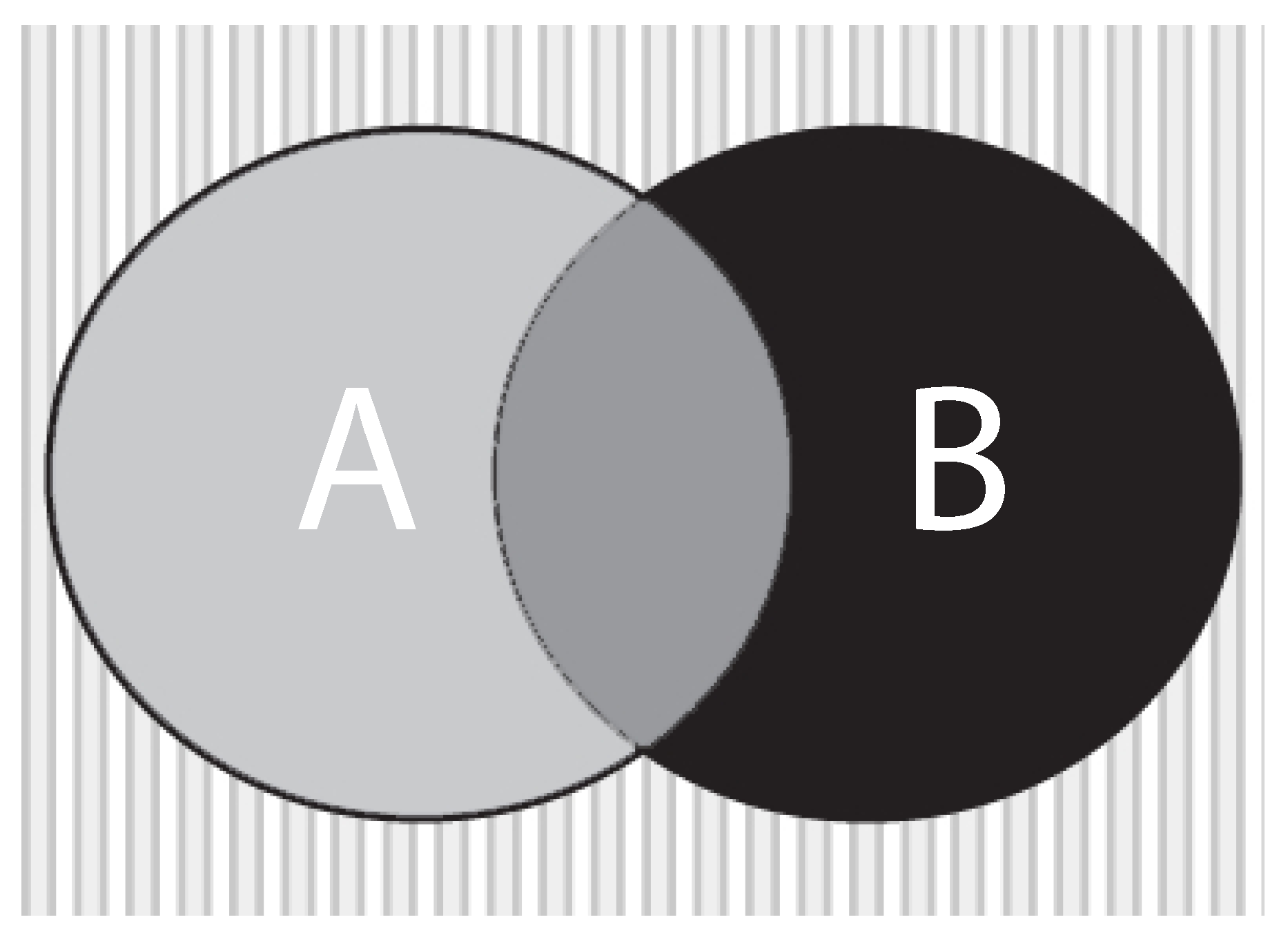
Figure 6.
Diagrams classifying entanglement with density matrices. Left: An non-factorizable or entangled system with a generic probe . Right: A separable system conditional upon a special class of probe is also called factorized.
Figure 6.
Diagrams classifying entanglement with density matrices. Left: An non-factorizable or entangled system with a generic probe . Right: A separable system conditional upon a special class of probe is also called factorized.

Publisher’s Note: MDPI stays neutral with regard to jurisdictional claims in published maps and institutional affiliations. |
© 2022 by the author. Licensee MDPI, Basel, Switzerland. This article is an open access article distributed under the terms and conditions of the Creative Commons Attribution (CC BY) license (https://creativecommons.org/licenses/by/4.0/).
Share and Cite
MDPI and ACS Style
Ralston, J.P. What Can We Learn from Entanglement and Quantum Tomography? Physics 2022, 4, 1371-1383. https://doi.org/10.3390/physics4040088
AMA Style
Ralston JP. What Can We Learn from Entanglement and Quantum Tomography? Physics. 2022; 4(4):1371-1383. https://doi.org/10.3390/physics4040088
Chicago/Turabian StyleRalston, John P. 2022. "What Can We Learn from Entanglement and Quantum Tomography?" Physics 4, no. 4: 1371-1383. https://doi.org/10.3390/physics4040088