Article

Generalized Extended Uncertainty Principle Black Holes: Shadow and Lensing in the Macro- and Microscopic Realms

by
Nikko John Leo S. Lobos
1,2,* and
Reggie C. Pantig
2,3
1
Mathematics and Physics Department, Technological Institute of the Philippines, 363 Pascual Casal St., Manila 1001, Philippines
2
Physics Department, De La Salle University, 2401 Taft Avenue, Manila 1004, Philippines
3
Physics Department, Mapúa Institute of Technology, 658 Muralla St., Intramuros, Manila 1002, Philippines
*
Author to whom correspondence should be addressed.
Physics 2022, 4(4), 1318-1330; https://doi.org/10.3390/physics4040084
Submission received: 1 August 2022 / Revised: 5 October 2022 / Accepted: 8 October 2022 / Published: 28 October 2022
(This article belongs to the Special Issue New Advances in Quantum Geometry)

Abstract

:
Motivated by the recent study about the extended uncertainty principle (EUP) black holes, we present in this study its extension called the generalized extended uncertainty principle (GEUP) black holes. In particular, we investigated the GEUP effects on astrophysical and quantum black holes. First, we derive the expression for the shadow radius to investigate its behavior as perceived by a static observer located near and far from the black hole. Constraints to the large fundamental length scale, L * , up to two standard deviations level were also found using the Event Horizont Telescope (EHT) data: for black hole Sgr. A*, L * = 5.716 × 10 10 m, while for M87* black hole, L * = 3.264 × 10 13 m. Under the GEUP effect, the value of the shadow radius behaves the same way as in the Schwarzschild case due to a static observer, and the effect only emerges if the mass, M, of the black hole is around the order of magnitude of L * (or the Planck length, l Pl ). In addition, the GEUP effect increases the shadow radius for astrophysical black holes, but the reverse happens for quantum black holes. We also explored GEUP effects to the weak and strong deflection angles as an alternative analysis. For both realms, a time-like particle gives a higher value for the weak deflection angle. Similar to the shadow, the deviation is seen when the values of L * and M are close. The strong deflection angle gives more sensitivity to GEUP deviation at smaller masses in the astrophysical scenario. However, the weak deflection angle is a better probe in the micro world.

1. Introduction

Black hole theory has never been more exciting than before when the Event Horizon Telescope (EHT) Collaboration revealed the first image of a black hole in M87 galaxy [1], and more recently, the black hole Sgr. A* in our galaxy [2]. These pictures, with very special algorithms, provided further evidence that black holes exist in nature. Black holes are compact objects with gravity so strong that not even light can escape its gravitational grip.
Black hole solutions are found by solving the Einstein field equation, and the simplest black hole model that is static and spherically symmetric was found by Karl Schwarzschild [3] (see [4] for English translation). Later on, the metric of a spinning black hole, which is static and axisymmetric, was found by Roy Kerr [5]. Conceptually, black holes are massive objects where all the mass is concentrated into a point, thus giving the object an infinite density. In essence, there is no doubt that there must be some interplay between gravity and quantum mechanics in these extreme regions. Indeed, black holes are laboratories where one can probe the quantum nature of gravity [6].
Central to the microscopic realm is the Heisenberg uncertainty principle (HUP), which states that
Δ x Δ p / 2 ,
which is derived from the commutation relation of the position, x ^ , and momentum, p ^ , operators, with the reduced Planck’s constant. That is, [ x ^ , p ^ ] = i . Equation (1) can provide limitations in testing predictions, but nonetheless a hypothetical energy probe can still detect very short distance scales. The main problem is that, beyond the Planck length, l Pl , there is no guarantee that the spacetime observed is still smooth. Such a chaotic spacetime in the microscopic realm is called the quantum foam [7]. It is only then that the HUP must be modified to accommodate the Planck length, and the most accepted modification is called the generalized uncertainty principle (GUP) [8,9,10], which adds uncertainty quadratic in momentum:
Δ x Δ p 1 + β l Pl 2 Δ p 2 ,
where β is a dimensionless quantity usually taken as unity and can be either positive or negative [11].
As nature is fond of symmetry and duality, similar to the yin-yang symbol, it is only natural to suspect that if there is a minimum fundamental length, there must be a large fundamental length scale in our Universe. Hence, the GUP is naturally extended [12], to include the large fundamental length, L * , through a quadratic correction in the position uncertainty. That is,
Δ x Δ p 1 + α Δ x 2 / L * 2 ,
which is commonly called the extended uncertainty principle (EUP), with α being another dimensionless constant. Equation (3) was also derived from first principles in Ref. [13]. While GUP is commonly analyzed in the literature due to its vast application in the microscopic world [14], the application of EUP seems to be dearth in the literature. For instance, the analysis of EUP effects on the thermodynamics of Friedmann–Robertson–Walker (FRW) Universe [15] was analyzed long ago and a year later applied to the geometry of de Sitter (dS) and anti-de Sitter (AdS) spacetime [16]. The effects of the EUP correction has also been studied in Rindler and cosmological horizons [17], relativistic Coulomb potential [18], bound-state solutions of the two-dimensional Dirac equation with Aharonov–Bohm–Coulomb interaction [19], Jüttner gas [20]. With the help of the GUP and EUP parameters, bounds for the Hubble parameter’s value were also studied to resolve the Hubble tension [21]. It is only recently that EUP correction has been applied in the context of black holes [22], with r h Δ x given the gravitons are considered the quantum particles inside such confinement. Since then, various studies have explored the black hole with EUP correction; see Refs. [23,24,25,26,27,28,29,30,31].
We are motivated to continue the analysis of Ref. [22] and further investigate the most general form of the uncertainty principle [32],
Δ x Δ p 1 + β l Pl 2 Δ p 2 + α Δ x 2 / L * 2 ,
as been applied to the shadow cast and gravitational lensing of astrophysical black holes and quantum black holes [33,34]. To this end. the black hole metric that contains the GEUP correction must be expressed as (in time and cylindrical space coordiantes) [22]
d s 2 = A ( r ) d t 2 + B ( r ) d r 2 + C ( r ) d θ 2 + D ( r ) d ϕ 2 ,
where
A ( r ) = 1 2 M r , B ( r ) = A ( r ) 1 , C ( r ) = r 2 , D ( r ) = r 2 sin 2 θ .
With the GEUP correction in Equation (4), the mass, M, of the black hole corrected to [22]:
M = M 1 + 4 α M 2 L * 2 + β 2 M 2 .
Here, we first show to emphasize the quantum correction for quantum particles. Note that, since M is geometrized, one can relate to the Planck length representing the known minimal length l Pl = 1.616 × 10 35 m . Furthermore, α = β = 1 , and L * ’s value is estimated based on the observational constraints from the EHT in Section 2. First, we explore the behavior of the shadow radius of the object being considered (i.e., supermassive black hole (SMBH) for macroscopic and some elementary particles for the microscopic realm). Shadows are important since they can reveal imprints that allow one to test gravity theories in the strong field regime; shadows were first studied in Ref. [35]. In 1979, Luminet gave the formula for the angular radius of the shadow [36]. Then several studies have explored the shadows of quantum black holes [37,38,39,40,41,42,43,44]. In this paper, we are also interested in probing the GEUP effects using the strong and weak deflection angles. Gravitational lensing is one of the most successful tools as it verified Einstein’s general theory of relativity in 1919 [45] through the Sun’s solar eclipse. Since then, it has been crucial in probing various tests of gravitation theories. Several tools have been developed [46,47,48], and in 2008, the Gauss–Bonnet theorem on the optical geometries in asymptotically flat spacetimes was developed [49]. It was extended by Werner [50] to include stationary spacetimes in the Finsler–Randers type optical geometry on Nazim’s osculating Riemannian manifolds. Ishihara and others then found a way to extend the Gauss-Bonnet theorem (GBT) to incorporate finite distance effects [51,52], which also applies to non-asymptotic spacetimes. Finally, instead of using points at infinity as integration domain for the GBT, the study in [53] used the photonsphere to naturally find an alternative to the Ishihara method, which also accommodates the deflection angle of massive particles. For recent works about quantum black holes’ deflection angles, see Refs. [24,29,54,55,56,57,58].
The paper is organized as follows. Section 2 is devoted to exploring the shadow behavior of the GEUP black hole and microscopic entities been viewed as quantum black holes. In Section 3, the Gauss–Bonnet theorem is used to study the weak deflection angle of the mentioned objects. Section 4 considers the strong deflection angle as a generalization of the weak deflection angle studied in Section 3. Then, in Section 5, we formulate the conclusion based on the results of the prior Sections. In this paper, geometrized units are used wherein G = c = 1 , with G being the gravitaion constant and c the speed of light, and the metric signature ( , + , + , + ); hence, in Equation (7) can be replaced by the Planck length.

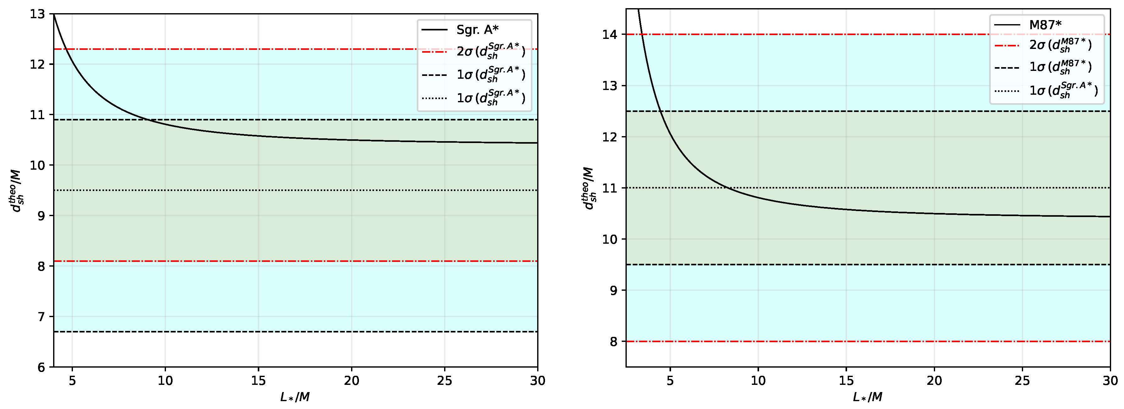
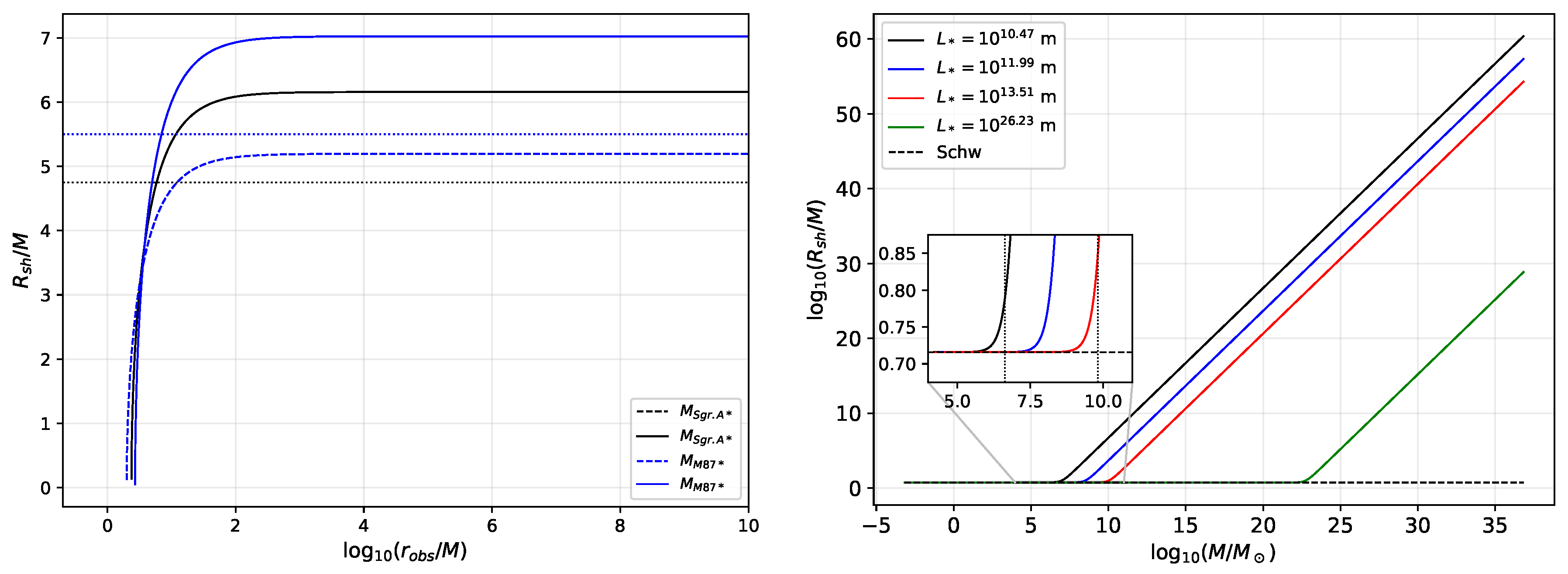
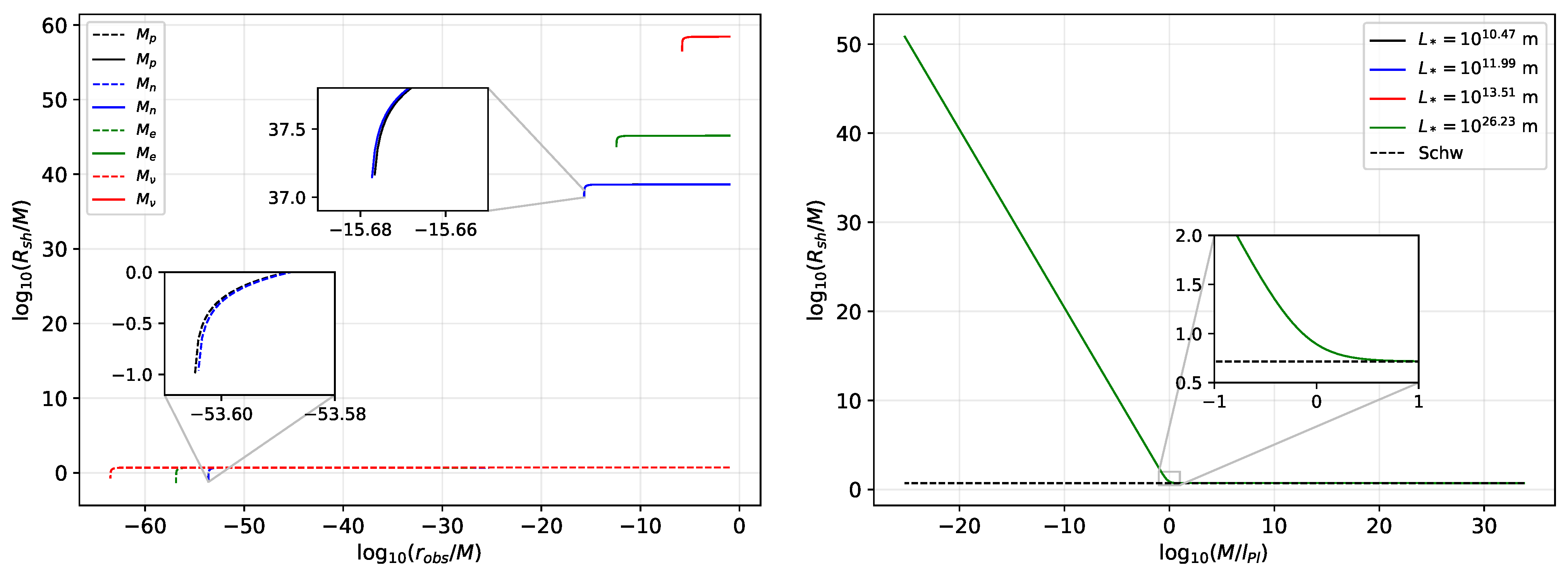
2. Shadow and Constraints to the Large Fundamental Length Scale

In this Section, we study the shadow of the GEUP black hole. Thanks to r and t independence of the metric, such symmetry allows us to analyze light-like geodesics along the equatorial plane ( θ = π / 2 ) without compromising generality. Thus, D ( r ) = C ( r ) in the metric (5). These geodesics can be derived through the Lagrangian,
L = 1 2 A ( r ) t ˙ + B ( r ) r ˙ + C ( r ) ϕ ˙ .
Here on, the dot denotes the time derivation.
Through the variational principle, the Euler–Lagrange equation gives two constants of motion
E = A ( r ) d t d λ , L = C ( r ) d ϕ d λ ,
from where one can define the impact parameter as
b L E = C ( r ) A ( r ) d ϕ d t .
Here, λ denotes the affine parameter defined by τ = μ λ , where τ is the proper time and μ is the particle’s rest mass.
For light-like geodesics, the metric can be set as d s 2 = 0 , and using Equation (9), one obtains the orbit equation:
d r d ϕ 2 = C ( r ) B ( r ) h ( r ) 2 b 2 1 ,
where by definition [59],
h ( r ) 2 = C ( r ) A ( r ) .
Through the above equation, we can obtain the location of the photonsphere by taking h ( r ) = 0 , where the prime denotes r-derivation. To this end, since the mass M is just imbued with quantum correction, the location of the photonsphere is
r ph = 3 M .
Our concern in this Section is how the observer will perceive the GEUP black hole at near and far away locations. Let the observer be at the coordinates ( t obs , r obs , θ obs = π / 2 , ϕ obs = 0 ) . Then, the observer can construct [60] the relation,
tan ( α sh ) = lim Δ x 0 Δ y Δ x = C ( r ) B ( r ) 1 / 2 d ϕ d r | r = r obs ,
which can be rewritten as
sin 2 ( α sh ) = b crit 2 h ( r obs ) 2 ,
where b crit is a function of the photonsphere given in Equation (13). A spacetime may have a different expression for h ( r ) , thus for a general spacetime, the critical impact parameter reads [61]:
b crit 2 = h ( r ph ) B ( r ph ) C ( r ph ) B ( r ph ) C ( r ph ) [ h ( r ph ) B ( r ph ) C ( r ph ) h ( r ph ) B ( r ph ) C ( r ph ) 2 h ( r ph ) B ( r ph ) C ( r ph ) ] ,
and, for the GEUP black hole, one finds:
b crit 2 = 27 M 2 .
Finally, one obtains the behavior of the shadow radius, applicable for both macroscopic and quantum black holes:
R sh = 3 M 3 1 2 M r obs .
Note that this expression is valid even when the static observer is near the black hole. In addition, if r obs , Equation (18) can be approximated with R sh = 3 3 M .
Let us start first with astrophysical black holes, such as Sgr. A* and M87*, and discuss some observational constraints. According to Refs. [1,2], the mass ( M denotes the mass of the Sun), distance from Earth, and angular shadow diameter of M87* are [62]: M M 87 * = 6.5 ± 0.90 × 10 9 M , D = 16.8 Mpc, and α M 87 * = 42 ± 3 μ as, respectively. For Sgr. A*, these values are: M Sgr . A * = 4.3 ± 0.013 × 10 6 M (Very Large Telescope Interferometer, VLTI), D = 8277 ± 33 pc, and α Sgr . A * = 48.7 ± 7 μ as (EHT), respectively [1,2]. The diameter of the shadow size using these empirical data and in units of the black hole mass can be calculated using
d sh = D θ / M .
Then, the diameter of the shadow image of M87* and Sgr. A* are d sh M 87 * = ( 11 ± 1.5 ) M , and d sh Sgr .   A * = ( 9.5 ± 1.4 ) M , respectively. Meanwhile, the theoretical shadow diameter can be obtained as d sh theo = 2 R sh . The observational constraints’ results are plotted in Figure 1.
Theoretically, let us now consider how the static observer perceives the shadow radius at different locations in the radial coordinate for different values of L * . In the literature, only the case of r obs were considered [22,29].
In Figure 2, left plot, the dashed line is the Schwarzschild case for both SMBHs, which overlaps the shadow radius coming from empirical data [1,2] shown for comparison. Note that the GEUP effect merely increases the shadow radius while the trend of the behaviour of the curve is the same as in the Schwarzschild case. In the right plot, one can see how the shadow radius behaves due to the GEUP effect. For instance, deviations begin to manifest if the value of L * is close to the mass of the black hole, which is also visible from the green line as soon as L * comparable to the Hubble length is used. In this scenario, the effect of the parameters in the microscopic realm does not even manifest.
Equation (18) also admits analysis for quantum black holes. The results are plotted in Figure 3.
The left plot shows the case where the static observer may be represented by a detector that can probe masses as small as the proton, neutron, electron, and neutrino [63], where their geometrized masses are used. The dashed and solid lines represent the Schwarzschild and GEUP cases, respectively. The right plot reveals that L * is indeed irrelevant in the microscopic realm. Nonetheless, with the GUP correction, the plot reveals the detector’s position where the shadow of the particle manifests. Take, for example, the neutrino. Without GUP correction, the shadow radius is around 10 63 order of magnitude for a wide range of detector locations. The GUP correction lessens this range and makes the shadow radius larger. For instance, if the detector is at r = 1.59 × 10 67 m, then the shadow radius is around R sh = 5.03 × 10 6 m. Note how the shadow radius of these particles levels at greater distances. Finally, one observes that, without GUP correction, the shadow radii are nearly identical to each other. With the GUP correction, we have seen that, as the mass of the particle decreases, the shadow radius tends to increase while the range where a detector can observe it decreases.

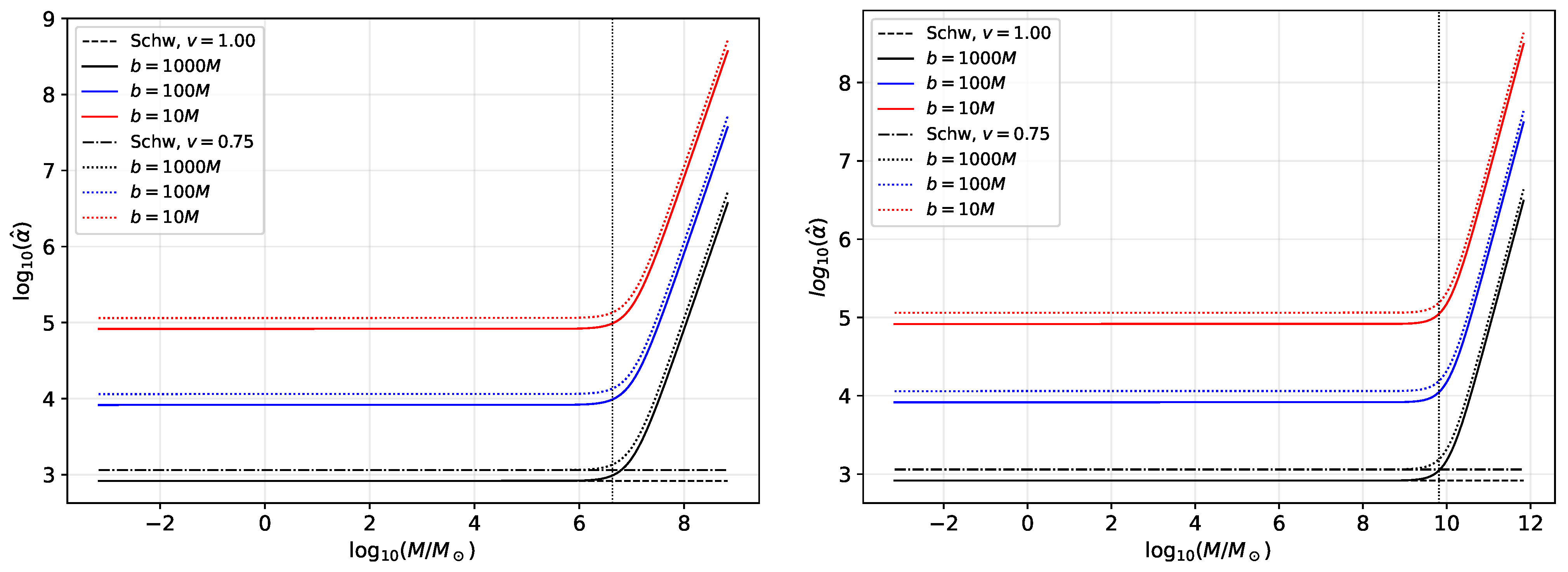
3. Weak Deflection Angle

In this Section, we explore a different phenomenon and examine the effect of the GEUP correction on the weak deflection angle by black holes in the macroscopic and microscopic realms. To do so, we use the GBT. Consider the domain ( D a , g ¯ ) (where a = 1 , 2 , . . . , N and g ¯ is the optical geometry metric) that is connected over an osculating Riemannian manifold ( M , g ¯ ) along some boundaries, and let κ g be the geodesic curvature of the boundary D a . Then the GBT states that [49,64]
D a K d S + a = 1 N D a κ g d + a = 1 N θ a = 2 π χ ( D a ) ,
where χ ( D a ) is the Euler characteristic, K is the Gaussian optical curvature, d S = g d r d ϕ , denotes the line element, and θ a is the exterior angle at the Nth vertex.
Although the spacetime herein is asymptotically flat under the GEUP correction, we used the generalized GBT that considers non-asymptotically flat spacetime and massive particle deflection. In Ref. [53], the photonsphere radius r ph is the one considered as part of the quadrilateral for integration domain. It is shown that the weak deflection angle,
α ^ = r ph R r ph S K d S + ϕ RS ,
where integral is taken over through r ph S R r ph Here, S and R are the radial positions of the source and receiver, respectively, and ϕ RS is the coordinate position angle between the source and the receiver defined as ϕ RS = ϕ R ϕ S . g is the determinant of the Jacobi metric in static and spherically symmetric spacetime:
d l 2 = g i j d x i d x j = ( E 2 μ 2 A ( r ) ) B ( r ) A ( r ) d r 2 + C ( r ) A ( r ) d Ω 2 .
Here, E is the energy of the massive particle defined by
E = μ / 1 v 2 ,
where v is the particle’s velocity. As only the equatorial plane is considered here due to spherical symmetry, the determinant of the Jacobi metric reads:
g = B ( r ) C ( r ) A ( r ) 2 ( E 2 μ 2 A ( r ) ) 2 .
Following Ref. [53], one obtains the final expression for the weak deflection angle:
α ^ M v 2 + 1 b v 2 1 b 2 u R 2 + 1 b 2 u S 2
which also involves the finite distance u S and u R . The obtained expression for α ^ can still be further approximated as soon as b 2 u 2 0 :
α ^ 2 M v 2 + 1 b v 2
For the case of photons, when v = 1 , one finds:
α ^ 4 M / b .
The weak deflection angle result is usually applied to SMBH. As soon as α ^ is usually plotted against the impact parameter b / M , in Figure 4 we are interested how α ^ changes as the black hole mass under the effect of GEUP varies. Without the GEUP correction, the plot would only represent straight lines. From Figure 4, one observes that similar to the shadow radius, the deviation occurs when M is close to the value of L * . The time-like deflection also produces a higher value of α ^ , and the lower the impact parameter, the greater the deflection. Note that in this plot, b = 10 M is still in the regime for weak deflection angle since this is higher than the critical impact parameter, b crit = 3 3 M . We use this information for the weak deflection for quantum black holes and strong deflection angle.
As a final remark to the plots is that showing how α ^ changes as the mass M varies has its shortcomings since b / M is constant. For instance, if one considers the mass of the Earth, b = 1000 M equals 4.4 m, which is too small compared to the radius of the Earth (6371 km). Thus, the line plot in Figure 4 may have its range of validity relative to the chosen value of the impact parameter. Such a result has a critical implication as far as the GEUP model in this study is concerned. One can verify that if the dimensional reduction is used in the metric in Equation (7) to calculate α ^ , that is when l Pl = 1 [22], one can observe a very high value for α ^ for low mass compact objects (such as Earth, for example).
We also apply the weak deflection angle for quantum black holes [33,34]. We do this by plotting α ^ versus log 10 ( M / l Pl ) in Figure 5. Let us note that when one geometrizes the Planck mass, the Planck length is obtained, so, for simplicity, α ^ is plotted in terms of M / l Pl in Figure 5. Qualitatively, from Figure 5, one observes the same features as those are known for the weak deflection for astrophysical black holes. Here, one can see that the deviation begins to manifest when the log 10 ( M / l Pl ) 0 , and these are the masses that are comparable with l Pl (∼ 2.176 × 10 8 kg in metric units). In this case, α ^ 114,815 μas and can be detectable if one directs a photon at an impact parameter of b 1.62 × 10 32 m. Such particle is still massive, and its physical dimension may cause a collision instead of a deflection. Weak deflection may occur unless the particle is compressed to allow such a small value for the impact parameter. In the plot shown, the vertical dotted line represents the neutrino’s mass. One can see that α ^ 3.89 × 10 60 μ as for b = 1000 M . Such a large weak deflection angle can be made smaller by increasing b. However, the main obstacle in this case is that one cannot observe neutrinos at rest.

4. Strong Deflection Angle

Near the black hole region, specifically in the critical impact parameter, the deflection angle is described by the strong deflection expression as shown in Refs. [48,65,66]. The photonsphere region is crucial in strong deflection calculation; hence, we use Equation (13). Following Refs. [48,65,66], one obtains the strong deflection angle to read:
α ^ str = a ¯ ln b 0 / b crit 1 + b ¯ + O ( b b crit ) ,
where a ¯ and b ¯ are the coefficients of strong deflection and b 0 and b crit correspond to the impact parameters evaluated at the closest approach and critical impact parameter, respectively. The coefficients of the strong deflection are calculated based on Ref. [65], namely:
a ¯ = 2 B ( r ph ) C ( r ph ) C ( r ph ) A ( r ph ) A ( r ph ) C ( r ph ) ,
and
b ¯ = a ¯ ln r ph C ( r ph ) C ( r ph ) A ( r ph ) A ( r ph ) + I R ( r ph ) π ,
where A ( r ph ) , B ( r ph ) , and C ( r ph ) are metric functions evaluated at the photon sphere region, and I R denotes the regular integral evaluated from 0 to 1. The double prime signifies second derivative with respect to r evaluated at the photonsphere, r r ph .
The second term in Equation (30) can be calculated using the procedure illustrated in [65,66], where
I R ( r ph ) = 0 1 2 ( 1 A ph ) A ( z , r ph ) B ( z , r ph ) A ( z , r ph ) C ( z , r ph ) A ph / C ph A ( z , r ph ) / C ( z , r ph ) d z ,
and A ( z , r ph ) , B ( z , r ph ) , and C ( z , r ph ) are metric functions A ( r ) , B ( r ) , and C ( r ) evaluated using the new variable [65],
z 1 r ph / r .
Let us express Equation (32) in terms of r and substitute it to the metric functions. Applying the expression in Equations (29)–(31) to the black hole metric (5), one finds:
a ¯ = 1 ,
and
b ¯ = ln 216 ( 7 4 3 ) π .
When α and β are set to zero, the Schwarzschild expression is retrieved for strong deflection [67]:
α ^ str = ln b / b crit 1 0.40023 ,
with the critical impact parameter from Equation (16) [61], resulting to Equation (17). In choosing the value of b it is essential to note that the ratio, b / b crit , must not be significantly far from 1. Equation (35) diverges for b crit = b . This shows that the photonsphere captures particles in this region. In the plots shown below in Figure 6 and Figure 7, b (in units of M) is chosen to be slightly larger than b crit = 3 3 M . We plot the strong deflection angle demonstarting how GEUP affects astrophysical and quantum black holes.
Figure 6 shows that the strong deflection angle curves are steeper than the weak deflection angle. While one observes the same feature of the low impact parameter producing higher deflection angle, one can see that the deviations due to the GEUP in the strong deflection regime occur early (at lower mass) than that obsreved for the weak deflection angle (cf. Figure 4), thus providing with an enhanced detectability.
Due to Equation (35), there is some value for mass M where the strong deflection ceases, and this value is near the value of the GEUP parameters L * and l Pl (see also Figure 7). Without the influence of GEUP, the strong deflection angle seems to have no limit for any values of mass M (as shown by the dashed black line). The same feature can be observed for quantum black holes. Again, while strong deflection is theoretically possible for small particles, a problem in its detectability is looming in the impact parameters, b, since it might be small compared to the particle’s physical dimension.

5. Conclusions

While the effects of the generalized (GUP) and extended (EUP) uncertainty principles are commonly analyzed separately in the literature, our study in this paper is about unifying these two quantum corrections as applied to black hole physics. Motivated by the study of Ref. [22], we investigated the effect of GEUP on the shadow and lensing for astrophysical black holes and very small particles viewed as quantum black holes.
We first find constraints to the values of the fundamental length scale, L * , using astrophysical data from the Event Horizon Telescope (EHT) Collaboration. For the two standard deviations level of uncertainty, we found an upper bound, L * 2.985 × 10 10 m, for Sgr. A* and L * 3.264 × 10 13 m for M87* black holes. Interestingly, for M87*, there is a value for L * which crosses the mean of the shadow diameter, which is L * 7.950 × 10 13 m. We note that this order of magnitudes agrees with the constraints of gravitational lensing observables, position, magnification, and differential time delays in [23]. We also examined how the shadow radius behaves based on the position of the observer from the GEUP black hole. The results obtained indicate that a black hole with GEUP generally follows the same pattern for the shadow radius curve as that retained. in the Schwarzschild case. In particular, the GEUP parameter L * generally increases the shadow radius for black hole masses with the same order of magnitude as L * . We also did not find any influence of GUP on the shadow of astrophysical black holes. Shadows for quantum black holes are also investigated. Here, as the quantum black hole’s mass, M, under GEUP correction decreases, we found that quantum black hole’s corresponding shadow increases. The position of detectors also affects the radius of such shadows. Lastly, it is shown that L * does not affect the quantum black hole’s shadow.
Alternatively, we probe more into the effects of GEUP by considering the strong and weak deflection angles. For the weak deflection angle, the main result indicates that deviation caused by GEUP occurs when the masses are comparable to the fundamental length scales. Such a deviation occurs early at a strong deflection angle. Furthermore, due to the fundamental length scales, there is a limitation for the occurrence of strong deflection angle. For example, if hypothetically the deflection angle by a neutrino is observed, then strong deflection cannot be applied due to the limitations imposed by the Planck length, l Pl .
Nonetheless, the weak deflection angle is still a better probe since it can be applied for relatively high impact parameters. The drawback is that measurement may not be possible due to the quantum nature of a particle. Finally, as far as the GEUP model in this study is concerned, the strong and weak deflection angles cannot probe whether L * affects the quantum realm, and vice versa. Lowering the value of L * may give an interesting result, but it may have some implications in the astrophysical phenomena that might be ruled out by observation. In theory, this direction is worth investigating.

Author Contributions

Conceptualization, R.C.P.; methodology, R.C.P. and N.J.L.S.L.; software, N.J.L.S.L.; validation, R.C.P.; formal analysis, R.C.P. and N.J.L.S.L.; investigation, R.C.P. and N.J.L.S.L.; resources, R.C.P. and N.J.L.S.L.; data curation, R.C.P. and N.J.L.S.L.; writing—original draft preparation, N.J.L.S.L.; writing—review and editing, R.C.P.; visualization, R.C.P.; supervision, R.C.P. All authors have read and agreed to the published version of the manuscript.

Funding

This research received no external funding.

Data Availability Statement

Not applicable.

Acknowledgments

We would like to thank the anonymous reviewers for their useful comments and suggestions that helped to improve the paper. R.C.P. would like to acknowledge support by the COST Action CA18108—Quantum gravity phenomenology in the multi-messenger approach (QG-MM).

Conflicts of Interest

The authors declare no conflict of interest.

References

  1. Akiyama, K. et al. [Event Horizon Telescope Collaboration] First M87 Event Horizon Telescope results. I. The shadow of the supermassive black hole. Astrophys. J. Lett. 2019, 875, L1. [Google Scholar] [CrossRef]
  2. Akiyama, K. et al. [Event Horizon Telescope Collaboration] First Sagittarius A* event Horizon Telescope results. I. The shadow of the supermassive black hole in the center of the Milky Way. Astrophys. J. Lett. 2022, 930, L12. [Google Scholar] [CrossRef]
  3. Schwarzschild, K. Über das Gravitationsfeld eines Massenpunktes nach der Einsteinschen Theorie. Sitzungsber. Preuss. Akad. Wiss. Berl. Math. Phys. 1916, 1916, 189–196. Available online: https://www.jp-petit.org/Schwarzschild-1916-exterior-de.pdf (accessed on 1 October 2022).
  4. Schwarzschild, K. “Golden Oldie”: On the gravitational field of a mass point according to Einstein’s theory. Gen. Relat. Gravit. 2003, 35, 951–959. [Google Scholar] [CrossRef]
  5. Kerr, R.P. Gravitational field of a spinning mass as an example of algebraically special metrics. Phys. Rev. Lett. 1963, 11, 237–238. [Google Scholar] [CrossRef]
  6. Rovelli, C. Quantum Gravity; Cambridge University Press: Cambridge, MA, USA, 2004. [Google Scholar] [CrossRef]
  7. Wheeler, J.A. Geons. Phys. Rev. 1955, 97, 511–536. [Google Scholar] [CrossRef]
  8. Maggiore, M. Quantum groups, gravity, and the generalized uncertainty principle. Phys. Rev. D 1994, 49, 5182–5187. [Google Scholar] [CrossRef] [PubMed] [Green Version]
  9. Maggiore, M. A generalized uncertainty principle in quantum gravity. Phys. Lett. B 1993, 304, 65–69. [Google Scholar] [CrossRef] [Green Version]
  10. Maggiore, M. The algebraic structure of the generalized uncertainty principle. Phys. Lett. B 1993, 319, 83–86. [Google Scholar] [CrossRef] [Green Version]
  11. Amati, D.; Ciafaloni, M.; Veneziano, G. Can spacetime be probed below the string size? Phys. Lett. B 1989, 216, 41–47. [Google Scholar] [CrossRef]
  12. Bambi, C.; Urban, F.R. Natural extension of the generalized uncertainty principle. Class. Quant. Grav. 2008, 25, 095006. [Google Scholar] [CrossRef]
  13. Costa Filho, R.N.; Braga, J.P.M.; Lira, J.H.S.; Andrade, J.S., Jr. Extended uncertainty from first principles. Phys. Lett. B 2016, 755, 367–370. [Google Scholar] [CrossRef]
  14. Tawfik, A.; Diab, A. Generalized uncertainty principle: Approaches and applications. Int. J. Mod. Phys. D 2014, 23, 1430025. [Google Scholar] [CrossRef] [Green Version]
  15. Zhu, T.; Ren, J.-R.; Li, M.-F. Influence of generalized and extended uncertainty principle on thermodynamics of FRW universe. Phys. Lett. B 2009, 674, 204–209. [Google Scholar] [CrossRef] [Green Version]
  16. Mignemi, S. Extended uncertainty principle and the geometry of (anti)-de-sitter space. Mod. Phys. Lett. A 2010, 25, 1697–1703. [Google Scholar] [CrossRef]
  17. Dabrowski, M.P.; Wagner, F. Extended uncertainty principle for Rindler and cosmological horizons. Eur. Phys. J. C 2019, 79, 716. [Google Scholar] [CrossRef] [Green Version]
  18. Hamil, B.; Merad, M.; Birkandan, T. Effects of extended uncertainty principle on the relativistic Coulomb potential. Int. J. Mod. Phys. A 2021, 36, 2150018. [Google Scholar] [CrossRef]
  19. Hamil, B.; Merad, M.; Birkandan, T. Bound-state solutions of the two-dimensional Dirac equation with Aharonov–Bohm-Coulomb interaction in the presence of extended uncertainty principle. Phys. Scr. 2020, 95, 105307. [Google Scholar] [CrossRef]
  20. Moradpour, H.; Aghababaei, S.; Ziaie, A.H. A Note on effects of generalized and extended uncertainty principles on Jüttner gas. Symmetry 2021, 13, 213. [Google Scholar] [CrossRef]
  21. Aghababaei, S.; Moradpour, H.; Vagenas, E.C. Hubble tension bounds the GUP and EUP parameters. Eur. Phys. J. Plus 2021, 136, 997. [Google Scholar] [CrossRef]
  22. Mureika, J.R. Extended Uncertainty Principle black holes. Phys. Lett. B 2019, 789, 88–92. [Google Scholar] [CrossRef]
  23. Lu, X.; Xie, Y. Probing an Extended Uncertainty Principle black hole with gravitational lensings. Mod. Phys. Lett. A 2019, 34, 1950152. [Google Scholar] [CrossRef]
  24. Kumaran, Y.; Övgün, A. Weak deflection angle of extended uncertainty principle black holes. Chin. Phys. C 2020, 44, 025101. [Google Scholar] [CrossRef] [Green Version]
  25. Cheng, H.; Zhong, Y. Instability of a black hole with f (R) global monopole under extended uncertainty principle. Chin. Phys. C 2021, 45, 105102. [Google Scholar] [CrossRef]
  26. Hassanabadi, H.; Chung, W.S.; Lütfüoğlu, B.C.; Maghsoodi, E. Effects of a new extended uncertainty principle on Schwarzschild and Reissner–Nordström black holes thermodynamics. Int. J. Mod. Phys. A 2021, 36, 2150036. [Google Scholar] [CrossRef]
  27. Hamil, B.; Lütfüoğlu, B.C. The effect of higher-order extended uncertainty principle on the black hole thermodynamics. EPL (Europhys. Lett.) 2021, 134, 50007. [Google Scholar] [CrossRef]
  28. Ökcü, O.; Aydiner, E. Investigating bounds on the extended uncertainty principle metric through astrophysical tests. EPL (Europhys. Lett.) 2022, 138, 39002. [Google Scholar] [CrossRef]
  29. Pantig, R.C.; Yu, P.K.; Rodulfo, E.T.; Övgün, A. Shadow and weak deflection angle of extended uncertainty principle black hole surrounded with dark matter. Ann. Phys. 2022, 436, 168722. [Google Scholar] [CrossRef]
  30. Hamil, B.; Lütfüoğlu, B.C.; Dahbi, L. EUP-corrected thermodynamics of BTZ black hole. Int. J. Mod. Phys. A 2022, 37, 2250130. [Google Scholar] [CrossRef]
  31. Chen, H.; Hassanabadi, H.; Lütfüoğlu, B.C.; Long, Z.W. Quantum corrections to the quasinormal modes of the Schwarzschild black hole. arXiv 2022, arXiv:2203.03464. [Google Scholar] [CrossRef]
  32. Kempf, A.; Mangano, G.; Mann, R.B. Hilbert space representation of the minimal length uncertainty relation. Phys. Rev. D 1995, 52, 1108–1118. [Google Scholar] [CrossRef] [PubMed] [Green Version]
  33. Calmet, X.; Carr, B.; Winstanley, E. Quantum Black Holes; Springer Briefs in Physics; Springer: Berlin/Heidelberg, Germany, 2014. [Google Scholar] [CrossRef]
  34. Hawking, S. Gravitationally collapsed objects of very low mass. Mon. Not. R. Astron. Soc. 1971, 152, 75–78. [Google Scholar] [CrossRef] [Green Version]
  35. Synge, J.L. The escape of photons from gravitationally intense stars. Mon. Not. R. Astron. Soc. 1966, 131, 463–466. [Google Scholar] [CrossRef]
  36. Luminet, J.P. Image of a spherical black hole with thin accretion disk. Astron. Astrophys. 1979, 75, 228–235. Available online: https://adsabs.harvard.edu/full/1979A%26A....75..228L (accessed on 1 October 2022).
  37. Konoplya, R.A. Quantum corrected black holes: Quasinormal modes, scattering, shadows. Phys. Lett. B 2020, 804, 135363. [Google Scholar] [CrossRef]
  38. Hu, Z.; Zhong, Z.; Li, P.C.; Guo, M.; Chen, B. QED effect on a black hole shadow. Phys. Rev. D 2021, 103, 044057. [Google Scholar] [CrossRef]
  39. Tamburini, F.; Feleppa, F.; Thidé, B. Constraining the Generalized Uncertainty Principle with the light twisted by rotating black holes and M87*. Phys. Lett. B 2022, 826, 136894. [Google Scholar] [CrossRef]
  40. Devi, S.; S, A.N.; Chakrabarti, S.; Majhi, B.R. Shadow of quantum extended Kruskal black hole and its super-radiance property. arXiv 2021, arXiv:2105.11847. [Google Scholar] [CrossRef]
  41. Anacleto, M.A.; Campos, J.A.V.; Brito, F.A.; Passos, E. Quasinormal modes and shadow of a Schwarzschild black hole with GUP. Ann. Phys. 2021, 434, 168662. [Google Scholar] [CrossRef]
  42. Xu, Z.; Tang, M. Testing the quantum effects near the event horizon with respect to the black hole shadow. Chin. Phys. C 2022, 46, 085101. [Google Scholar] [CrossRef]
  43. Karmakar, R.; Gogoi, D.J.; Goswami, U.D. Quasinormal modes and thermodynamic properties of GUP-corrected Schwarzschild black hole surrounded by quintessence. arXiv 2022, arXiv:2206.09081. [Google Scholar] [CrossRef]
  44. Rayimbaev, J.; Pantig, R.C.; Övgün, A.; Abdujabbarov, A.; Demir, D. Quasiperiodic oscillations, weak field lensing and shadow cast around black holes in symmergent gravity. arXiv 2022, arXiv:2206.06599. [Google Scholar] [CrossRef]
  45. Dyson, F.W.; Eddington, A.S.; Davidson, C. A Determination of the deflection of light by the Sun’s gravitational field, from observations made at the total eclipse of May 29, 1919. Philos. Trans. R. Soc. Lond. A 1920, 220, 291–333. [Google Scholar] [CrossRef]
  46. Virbhadra, K.S.; Ellis, G.F.R. Schwarzschild black hole lensing. Phys. Rev. D 2000, 62, 084003. [Google Scholar] [CrossRef] [Green Version]
  47. Bozza, V.; Capozziello, S.; Iovane, G.; Scarpetta, G. Strong field limit of black hole gravitational lensing. Gen. Rel. Grav. 2001, 33, 1535–1548. [Google Scholar] [CrossRef]
  48. Bozza, V. Gravitational lensing in the strong field limit. Phys. Rev. D 2002, 66, 103001. [Google Scholar] [CrossRef] [Green Version]
  49. Gibbons, G.W.; Werner, M.C. Applications of the Gauss-Bonnet theorem to gravitational lensing. Class. Quantum Gravity 2008, 25, 235009. [Google Scholar] [CrossRef]
  50. Werner, M.C. Gravitational lensing in the Kerr-Randers optical geometry. Gen. Rel. Grav. 2012, 44, 3047–3057. [Google Scholar] [CrossRef] [Green Version]
  51. Ishihara, A.; Suzuki, Y.; Ono, T.; Kitamura, T.; Asada, H. Gravitational bending angle of light for finite distance and the Gauss-Bonnet theorem. Phys. Rev. D 2016, 94, 084015. [Google Scholar] [CrossRef] [Green Version]
  52. Ishihara, A.; Suzuki, Y.; Ono, T.; Asada, H. Finite-distance corrections to the gravitational bending angle of light in the strong deflection limit. Phys. Rev. D 2017, 95, 044017. [Google Scholar] [CrossRef]
  53. Li, Z.; Zhang, G.; Övgün, A. Circular orbit of a particle and weak gravitational lensing. Phys. Rev. D 2020, 101, 124058. [Google Scholar] [CrossRef]
  54. Xu, C.; Yang, Y. Determination of bending angle of light deflection subject to possible weak and strong quantum gravity effects. Int. J. Mod. Phys. A 2020, 35, 2050188. [Google Scholar] [CrossRef]
  55. Zhang, R.; Lin, J.; Huang, Q. Strong gravitational lensing for the quantum-modified Schwarzschild black hole. Int. J. Theor. Phys. 2021, 60, 387–396. [Google Scholar] [CrossRef]
  56. Fu, Q.M.; Zhang, X. Gravitational lensing by a black hole in effective loop quantum gravity. Phys. Rev. D 2022, 105, 064020. [Google Scholar] [CrossRef]
  57. Lu, X.; Xie, Y. Gravitational lensing by a quantum deformed Schwarzschild black hole. Eur. Phys. J. C 2021, 81, 627. [Google Scholar] [CrossRef]
  58. Jusufi, K.; Övgün, A.; Banerjee, A.; Sakallı, t.I. Gravitational lensing by wormholes supported by electromagnetic, scalar, and quantum effects. Eur. Phys. J. Plus 2019, 134, 428. [Google Scholar] [CrossRef] [Green Version]
  59. Perlick, V.; Tsupko, O.Y.; Bisnovatyi-Kogan, G.S. Influence of a plasma on the shadow of a spherically symmetric black hole. Phys. Rev. D 2015, 92, 104031. [Google Scholar] [CrossRef] [Green Version]
  60. Perlick, V.; Tsupko, O.Y.; Bisnovatyi-Kogan, G.S. Black hole shadow in an expanding universe with a cosmological constant. Phys. Rev. D 2018, 97, 104062. [Google Scholar] [CrossRef] [Green Version]
  61. Pantig, R.C.; Övgün, A. Testing dynamical torsion effects on the charged black hole’s shadow, deflection angle and greybody with M87* and Sgr A* from EHT. arXiv 2022, arXiv:2206.02161. [Google Scholar] [CrossRef]
  62. Nandi, K.K.; Izmailov, R.N.; Yanbekov, A.A.; Shayakhmetov, A.A. Ring-down gravitational waves and lensing observables: How far can a wormhole mimic those of a black hole? Phys. Rev. D 2017, 95, 104011. [Google Scholar] [CrossRef]
  63. Eitel, K. Direct neutrino mass experiments. Nucl. Phys. B Proc. Suppl. 2005, 143, 197–204. [Google Scholar] [CrossRef]
  64. do Carmo, M. Riemannian Geometry; Birkhäuser: Boston, MA, USA, 1992. [Google Scholar]
  65. Tsukamoto, N. Deflection angle in the strong deflection limit in a general asymptotically flat, static, spherically symmetric spacetime. Phys. Rev. D 2017, 95, 064035. [Google Scholar] [CrossRef] [Green Version]
  66. Zhao, S.S.; Xie, Y. Strong deflection gravitational lensing by a modified Hayward black hole. Eur. Phys. J. C 2017, 77, 1–10. [Google Scholar] [CrossRef] [Green Version]
  67. Bisnovatyi-Kogan, G.S.; Tsupko, O.Y. Strong gravitational lensing by Schwarzschild black holes. Astrophysics 2008, 51, 99–111. [Google Scholar] [CrossRef]
Figure 1. Observational contraints for the M-normalized theoretical shadow diameter for various M-normalized fundamental length scales, L * , for black holes Sgr. A* and M87*, where M is the black hole mass. (Left): one standard deviation (1 σ ) for L * 5.716 × 10 10 m, 2 σ for L * 2.985 × 10 10 m. (Right): 1 σ for L * 4.224 × 10 13 m, 2 σ for L * 3.264 × 10 13 m. At the mean, L * 7.950 × 10 13 m.
Physics 04 00084 g001
Figure 2. (Left): the shadow radius of Sgr. A* and M87* with observer location dependency. The dashed line represents the Schwarzschild case and the solid line for the general extended uncertainty principle (GEUP) case. The horizontal black and blue dotted lines represent the shadow radius of Sgr. A* and M87* based on the Event Horizon Telescope (EHT) data [1,2]. (Right): the shadow radius as a function of the black hole mass. The black and blue vertical lines in the inset plot represent the mass of the Sgr. A* and M87*, respectively. “Schw” denotes the Schwarzild case and M denotes the mass of the Sun.
Physics 04 00084 g002
Figure 3. (Left): Observer-dependent shadow radius of some elementary particles: proton (p), neutron (n), electron (e), and neutrino ( ν ). (Right): The shadow radius plotted under the assumption that the observer/detector is at r obs M , where M is the quantum black hole’s mass, for different values of L * . The overlapping of these lines means that L * has no effect in the microscopic realm. l Pl denotes the Planck mass.
Physics 04 00084 g003
Figure 4. Weak deflection angle by Sgr. A* (Left), and M87* (Right) for different values of impact parameter. The vertical dotted line is the mass of the black hole considered. See text for details.
Physics 04 00084 g004
Figure 5. Weak deflection angle by quantum black hole. The red vertical dotted line corresponds to the mass of neutrino.
Physics 04 00084 g005
Figure 6. Behavior of strong deflection angle by Sgr. A* (Left) and M87* (Right). The black vertical dotted line is the corresponding mass of the supermassive black hole (SMBH). See text for details.
Physics 04 00084 g006
Figure 7. Strong deflection angle by quantum black holes.
Physics 04 00084 g007
Publisher’s Note: MDPI stays neutral with regard to jurisdictional claims in published maps and institutional affiliations.

