Bounds on Energies and Dissipation Rates in Forced Dynamos


Department of Applied Mathematics and Theoretical Physics (DAMTP), University of Cambridge, Clarkson Road, Cambridge CB3 0WA, UK
†
Current address: King’s College, University of Cambridge, King’s Parade, Cambridge CB2 1ST, UK.
Physics 2022, 4(3), 933-939; https://doi.org/10.3390/physics4030061
Submission received: 11 July 2022
/
Revised: 10 August 2022
/
Accepted: 16 August 2022
/
Published: 23 August 2022
(This article belongs to the Special Issue Dedication to Professor Michael Tribelsky: 50 Years in Physics)
Abstract
:This paper is concerned with limits on kinetic and magnetic energies and dissipation rates in forced flows that lead to dynamo action and a finite amplitude magnetic field. Rigorous results are presented giving upper and lower limits on the values of these quantities, in a simple cubic geometry with periodic boundary conditions, using standard inequalities. In addition to the general case, results in the special case of the Archontis dynamo are presented, in which fields and flows are closely similar in much of the domain.
1. Introduction
This paper sets out some rigorous bounds on statistically steady dynamos driven by steady forcing. Such dynamos have been widely investigated by a number of authors; for a review with references see [1]. Of particular interest is the so-called Archontis dynamo [2,3] in which the magnetic field is almost aligned with the velocity field over much of the domain. In the latter case the velocity field and magnetic field can be almost steady with steady forcing while in other cases the fields and flows are disordered and aperiodic in time, so that averages over both space and time have to be assumed constant to make progress. This permits the construction of both upper and lower bounds on the time-averaged magnetic energy or dissipation, and the ratios of these quantities to their kinetic equivalents. A number of these results have been given elsewhere (see references in Section 3), but others are apparently novel. Some general results are given, and also more restrictive bounds that obtain (approximately) when the fields and flows are of Archontis type. The analysis shows results for the simple case where the magnetic Prandtl is unity and also where it is small, as found in laboratory fluids.
2. Methods
The analysis is performed using a number of known inequalities (Poincaré, Cauchy–Schwartz, Hölder, and others) that have a long history in the literature; while the bounds that are derived are only approximate in the sense that results for real flows will not be close to the extreme limits derived, they have the merit of being universal and are useful as a consistency check on any numerical computations. There have been a number of rigorous results derived for magnetic field growth due to prescribed flow; see, e.g., [4]. Here, flows that are driven by a steady space-periodic forcing are examined. Results are presented both for the flows and fields themselves, and for the Elsasser variables, defined as the sum and difference of the velocity and magnetic fields.
3. Governing Equations
We consider forced incompressible flow and dynamo generated magnetic field in a periodic box off side L. The forcing is also taken to be incompressible. As well as the velocity forcing we have the Lorenz force due to the magnetic field. The momentum Equation for and the induction equation for can be written in the dimensionless forms:
where , , (measured in Alfvén velocity units) , and (the magnetic Prandtl number), where is the kinematic viscosity, where L is the length scale of the system, and the magnetic diffusivity. The parameter R is defined such that , where is defined as an average over the periodic box. Thus, R plays the role of a Reynolds number or inverse viscosity. For simplicity, the assumption is made that the forcing is independent of time, and it is further supposed that all quantities are periodic over a box of side L. It is also supposed that , and that . (It may be checked that these averages do not change during the evolution of the system.) We are interested in a system in a statistically steady state, and define to be the time average of over time.
4. Results
4.1. No Magnetic Field
Equations (1) and (2) have solutions with . In that case we can can find bounds on the kinetic energy and viscous dissipation in terms of properties of . Defining , we have the following results, noting that in the chosen geometry.
4.1.1. Upper Bound
Multiplying Equation (1) by and averaging and use of the Cauchy and Poincaré inequalities gives
where is defined by , , so that one has the upper bound,
The last of these inequalities is shown, recalling that , by noting that
.
4.1.2. Lower Bound
Multiplying Equation (1) by and averaging, recalling that is independent of time, one obtains:
One can bound the terms on the left hand side using the above inequalities and the Hölder inequality to get (defining , where A is a constant):
4.2. Dynamo Inequalities
We now introduce the induction equation and the Lorentz force term and try to generalise the above results. These are now framed as inequalities on the magnetic energy and magnetic dissipation; we define , .
4.2.1. Upper Bound
4.2.2. Lower Bound
More surprising perhaps is the fact that the magnetic dissipation is bounded below, for given values of R and . Multiplying Equation (1) by , using Equation (8) and averaging, one finds:
Then by analogous methods to the non-magnetic case one finally obtains:
These results are related to those shown by Tilgner [7] in the context of the G.O. Roberts dynamo.
4.2.3. Dissipation Ratio
One can write these results alternately in terms of the ratio of magnetic to kinetic dissipation. Let ; then (here :
The largest possible value of of is given by the intersection of the boundary curves of the inequalities in Equation (11). Eliminating at the intersection, one finds:
appears to increase monotonically with R. For many liquid metals ; in that case, if , one must have .
4.3. The Archontis Dynamo
Now these results can be applied to the Archontis dynamo to get what are probably rather conservative estimates on the relation between R and necessary to sustain such a dynamo.
The original forcing function used by Archontis takes the form,
Then one can see that , , . For the Archontis dynamo, and so the boundary of the region in space, where this is possible, is given by putting both the expressions in Equation (11) equal to unity, giving the approximate inequality for such a dynamo:
Since, as previously noted, in many physical systems, it can be seen that Archontis type dynamos can occur only for large values of R for such systems.
4.4. Use of Elsasser Variables
One can instead use the Elsasser variables . The equations can be written
Then multiplying each equation by , one finds, in the statistically steady state:
Now defining and using similar inequalities to those in previous Sections, one finds:
or, dividing through,
As a check consider the non-magnetic case for which . For we reproduce an inequality similar to Equation (4). When one obtains a weaker result. One can find relations corresponding to Equation (10) by multiplying Equation (15) by and averaging, leading to
where . To understand what these inequalities imply consider the special case , and the Archontis forcing, where . Then Equations (18) and (19) become:
For the Archontis dynamo, we have that , say. It is straightforward to check, using the lower sign in Equation (20), that the smallest value of the ratio compatible with the above inequalities is , and so R has to be large for an Archontis type dynamo, as indeed is found in the experiments; see for example the detailed calculations for large R, described for in [8], (with large R corresponding to small in their notation).
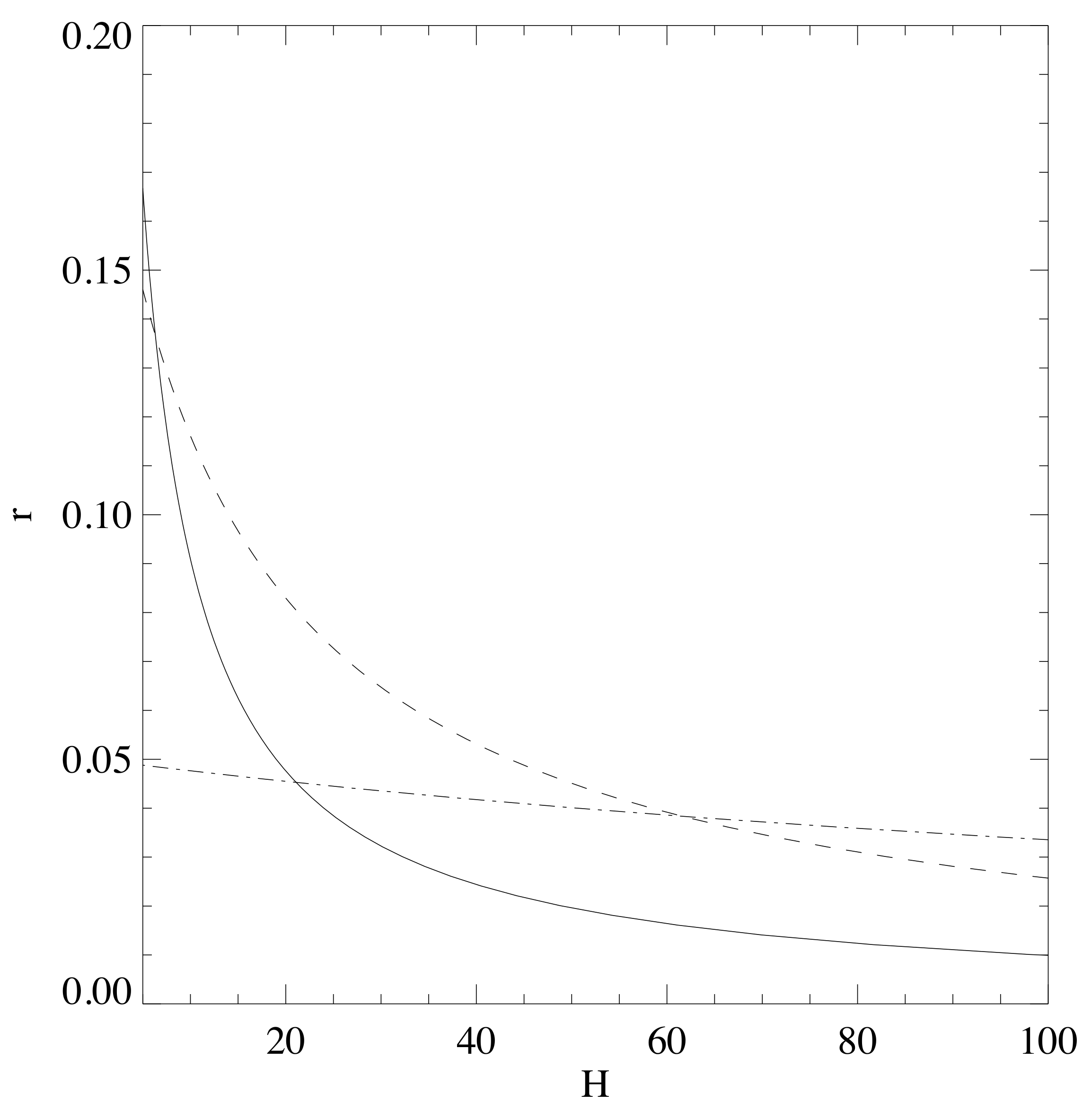
Similar results hold for general . Consider the interesting case . Then a similar calculation gives, for ,
How big should R - or - be to get close to the Archontis configuration? If then . If then and so has to be very large, of order , to reduce r significantly below .
Figure 1 shows the relation between and r for three values of . It can immediately be seen that as decreases (i.e., increases for fixed ) it becomes harder to make r small, i.e., to approach an Archontis state.
The values of k and r are not straightforwardly related. By use of the Schwartz inequality it can be established that as long as as envisaged one must have , so that, for instance, if r is close to zero, then k must be close to unity but, since r is bounded below rather than above for fixed , then k is not constrained.
5. Discussion
In this short paper, I explore the rigorous results that constrain the magnetic and kinetic energies and dissipation rates in a forced, fully nonlinear dynamo. It is possible to obtain both lower and upper bounds on the magnetic dissipation for a given forcing. In particular, the parameter R, which measures the amplitude of the forcing, has to be very large when the magnetic Prandtl number is small. Similar bounds can be found for the Elsasser variables, , and these lead to the same conclusion in the case of the Archontis dynamo where and are closely aligned in much of the domain, while some of the bounds are likely to be rather loose, they are at least rigorous, and provide guidance as to where in parameter space to look for exceptional configurations such as those found by Archontis. Work is in progress with D.J. Galloway to examine the accuracy of the bounds through direct numerical simulations. In Appendix A, the author of this paper presents his brief reminiscent about contacts with M. Tribelsky to whose honour this issue is dedicated.
Funding
This research was supported by a visiting Fellowship at the University of Sydney.
Data Availability Statement
Not applicable.
Acknowledgments
I am grateful to D.J. Galloway for hosting me at the University of Sydney and for helpful discussions.
Conflicts of Interest
The author declares no conflict of interest.
Appendix A
I am delighted to dedicate this paper to my friend and colleague Michael Tribelsky. I have known him since meeting in Bayreuth in 1989 at a conference and we had valuable discussions during his visit to the Isaac Newton Institute, Cambridge, UK in 2005.
Figure A1.
Michael Tribelsky (left) and Michael Proctor (right): Trinity College, Cambridge, UK in 2005.
Figure A1.
Michael Tribelsky (left) and Michael Proctor (right): Trinity College, Cambridge, UK in 2005.

References
- Galloway, D.J. Nonlinear dynamos. In Proceedings of the IAU Symposium No. 271: Astrophysical Dynamics: From Stars to Galaxies, 21–25 June 2010, Nice, France; Brummell, N.H., Brun, A.S., Miesch, M.S., Ponty, Y., Eds.; International Astronomical Union: Paris, France, 2011; pp. 297–303. [Google Scholar] [CrossRef]
- Archontis, V.; Dorch, S.B.F.; Nordlund, A. Nonlinear MHD dynamo operating at equipartition. Astron. Astrophys. 2007, 472, 715–726. [Google Scholar] [CrossRef]
- Dorch, S.B.F.; Archontis, V. On the saturation of astrophysical dynamos: Numerical experiments with the no-cosines flow. Sol. Phys. 2004, 224, 171–178. [Google Scholar] [CrossRef]
- Proctor, M.R.E. Introduction to dynamo theory. In Mathematical Aspects of Natural Dynamos; Dormy, E., Soward, A.M., Eds.; Chapman and Hall: New York, NY, USA; CRC Press: New York, NY, USA, 2007; pp. 20–41. [Google Scholar] [CrossRef]
- Doering, C.; Foias, C. Energy dissipation in body-forced turbulence. J. Fluid Mech. 2002, 467, 289–306. [Google Scholar] [CrossRef]
- Doering, C.; Eckhardt, B.; Schumacher, J. Energy dissipation in body-forced plane shear flow. J. Fluid Mech. 2003, 494, 275–284. [Google Scholar] [CrossRef]
- Tilgner, A. Scaling laws and bounds for the turbulent G.O. Roberts dynamo. Phys. Rev. Fluids 2017, 2, 024606. [Google Scholar] [CrossRef]
- Gilbert, A.D.; Ponty, Y.; Zheligovsky, V. Dissipative structures in a nonlinear dynamo. Geophys. Astrophys. Fluid Dyn. 2011, 105, 629–653. [Google Scholar] [CrossRef]
Figure 1.
The minimum value of as a function of for (solid line); (dashed line); (dash-dotted line). See text for details.
Figure 1.
The minimum value of as a function of for (solid line); (dashed line); (dash-dotted line). See text for details.

Publisher’s Note: MDPI stays neutral with regard to jurisdictional claims in published maps and institutional affiliations. |
© 2022 by the author. Licensee MDPI, Basel, Switzerland. This article is an open access article distributed under the terms and conditions of the Creative Commons Attribution (CC BY) license (https://creativecommons.org/licenses/by/4.0/).
Share and Cite
MDPI and ACS Style
Proctor, M. Bounds on Energies and Dissipation Rates in Forced Dynamos. Physics 2022, 4, 933-939. https://doi.org/10.3390/physics4030061
AMA Style
Proctor M. Bounds on Energies and Dissipation Rates in Forced Dynamos. Physics. 2022; 4(3):933-939. https://doi.org/10.3390/physics4030061
Chicago/Turabian StyleProctor, Michael. 2022. "Bounds on Energies and Dissipation Rates in Forced Dynamos" Physics 4, no. 3: 933-939. https://doi.org/10.3390/physics4030061