Article

Magnetic Resonance Velocimetry Measurement of Viscous Flows through Porous Media: Comparison with Simulation and Voxel Size Study

1
Institute of Fluid Mechanics, University of Rostock, 18059 Rostock, Germany
2
Department of Mechanical Engineering, University of Canterbury, Christchurch 8041, New Zealand
*
Author to whom correspondence should be addressed.
Physics 2021, 3(4), 1254-1267; https://doi.org/10.3390/physics3040079
Submission received: 29 October 2021 / Revised: 6 December 2021 / Accepted: 14 December 2021 / Published: 20 December 2021

Abstract

:
Studies that use magnetic resonance velocimetry (MRV) to assess flows through porous media require a sufficiently small voxel size to determine the velocity field at a sub-pore scale. The smaller the voxel size, the less information is lost through the discretization. However, the measurement uncertainty and the measurement time are increased. Knowing the relationship between voxel size and measurement accuracy would help researchers select a voxel size that is not too small in order to avoid unnecessary measurement effort. This study presents a systematic parameter study with a low-Reynolds-number flow of a glycerol–water mixture sent through a regularly periodic porous matrix with a pore size of 5 mm. The matrix was a 3-dimensional polymer print, and velocity-encoded MRV measurements were made at 15 different voxel sizes between 0.42 mm and 4.48 mm. The baseline accuracy of the MRV velocity data was examined through a comparison with a computational fluid dynamics (CFD) simulation. The experiment and simulation show very good agreement, indicating a low measurement error. Starting from the smallest examined voxel size, the influence of the voxel size on the accuracy of the velocity data was then examined. This experiment enables us to conclude that a voxel size of 0.96 mm, which corresponds to 20% of the pore size, is sufficient. The volume-averaged results do not change below a voxel size of 20% of the pore size, whereas systematic deviations occur with larger voxels. The same trend is observed with the local velocity data. The streamlines calculated from the MRV velocity data are not influenced by the voxel size for voxels of up to 20% of the pore size, and even slightly larger voxels still show good agreement. In summary, this study shows that even with a relatively low measurement resolution, quantitative 3-dimensional velocity fields can be obtained through porous flow systems with short measurement times and low measurement uncertainty.

1. Introduction

The development of an understanding of the flow through porous media is central to many fields of research and engineering [1,2,3,4]. However, the determination of local flow behavior has obvious experimental challenges: the matrix is often opaque and the matrix characteristics can change when it is observed in the absence of the fluid. Optical flow measurement techniques, such as laser Doppler velocimetry (LDV) and particle image velocimetry (PIV), require optical access to the flow field [5,6]. Furthermore, optical techniques require that the fluid and the solid matrix are transparent to light and that they share similar refractive indices. Magnetic resonance imaging (MRI), as a non-optical, non-invasive technique, does not suffer from these restrictions.
In velocity-encoded phase-contrast magnetic resonance imaging (MRI), which is referred to as magnetic resonance velocimetry (MRV), the pore network structure, including the fluid flow, can be measured at a sub-pore scale [7]. Typical MRV studies of porous media have involved measuring the flow of fluid through packed beds [8,9,10,11,12,13], rock cores [14] and open-celled foams [15].
With MRI and MRV, the field of view (FOV) is divided into uniformly sized volume elements, termed voxels. The smaller the voxel size, the less information is lost through the discretization. However, below a certain voxel size, the additional measurement effort is no longer proportional to the additional information obtained. The problem of discretization is particularly relevant for measurement in porous media. Most naturally occurring porous media is characterized by a range of length scales, and a decision has to be made as to which of these lengths the scales need to be fitted. A compromise between measurement accuracy and measurement time must be made.
Furthermore, a reduction in voxel size is not always possible. Besides the possible software and hardware limitations of the MRI system, a major limiting factor is the signal-to-noise ratio (SNR), which determines the measurement uncertainty of the velocity data. For a given system, the SNR is linearly dependent on the voxel volume and, therefore, weak SNR levels are quickly reached with decreasing voxel size. The loss in the SNR can be compensated for by averaging the signal, but since the SNR increases only with the square root of the sampling time, extreme numbers of averages would be necessary to improve a weak SNR. Knowing the relationship between voxel size and measurement accuracy would help when selecting a satisfactory voxel size that can avoid these issues while still resolving the flow field.
An obvious experimental advantage of MRV is that it can provide local velocity data at the interior of a porous medium as either an alternative to or as a verification of theoretical models. There are studies that offer comparisons between simulations and MRV, but these generally compare global variables (permeability, for example) [16]. There are few instances of direct local velocity comparisons between MRV and computational fluid dynamics (CFD) simulations, and these use higher resolution MRI. Using a uniform voxel size of 39.06 µm, a high resolution MRV study of flow through a packed bed of uniform polystyrene beads was conducted in Ref. [17], and the authors present local comparisons between the experimental and CFD-simulated velocities at five points on a plane perpendicular to the direction of the bulk flow. The authors of Ref. [18] do provide side-by-side local velocity comparisons between CFD and µPIV with a resolution of 1.73 μm/pixel. Such high resolutions can often not be accomplished with MRV for the reasons explained. The dependency between the voxel size and the accuracy of the experimental data is therefore a critical point when using MRV data to verify CFD simulations.
This study has two key aims. The first aim is to analyze the accuracy of MRV experiments involving porous media and to assess the velocity errors due to discretization (voxel size). Here, a controlled experiment is carried out with a highly structured porous sample with a uniform pore size. The laminar fluid flow through this sample is measured with different voxel sizes to study the dependency between voxel size and measurement error. The second aim of this study is to provide a side-by-side comparison between CFD and MRV of the local velocity profiles within the pore structure. Here, simulations are conducted using the fluid, flow, and geometry parameters reflecting those of the MRV experiment.

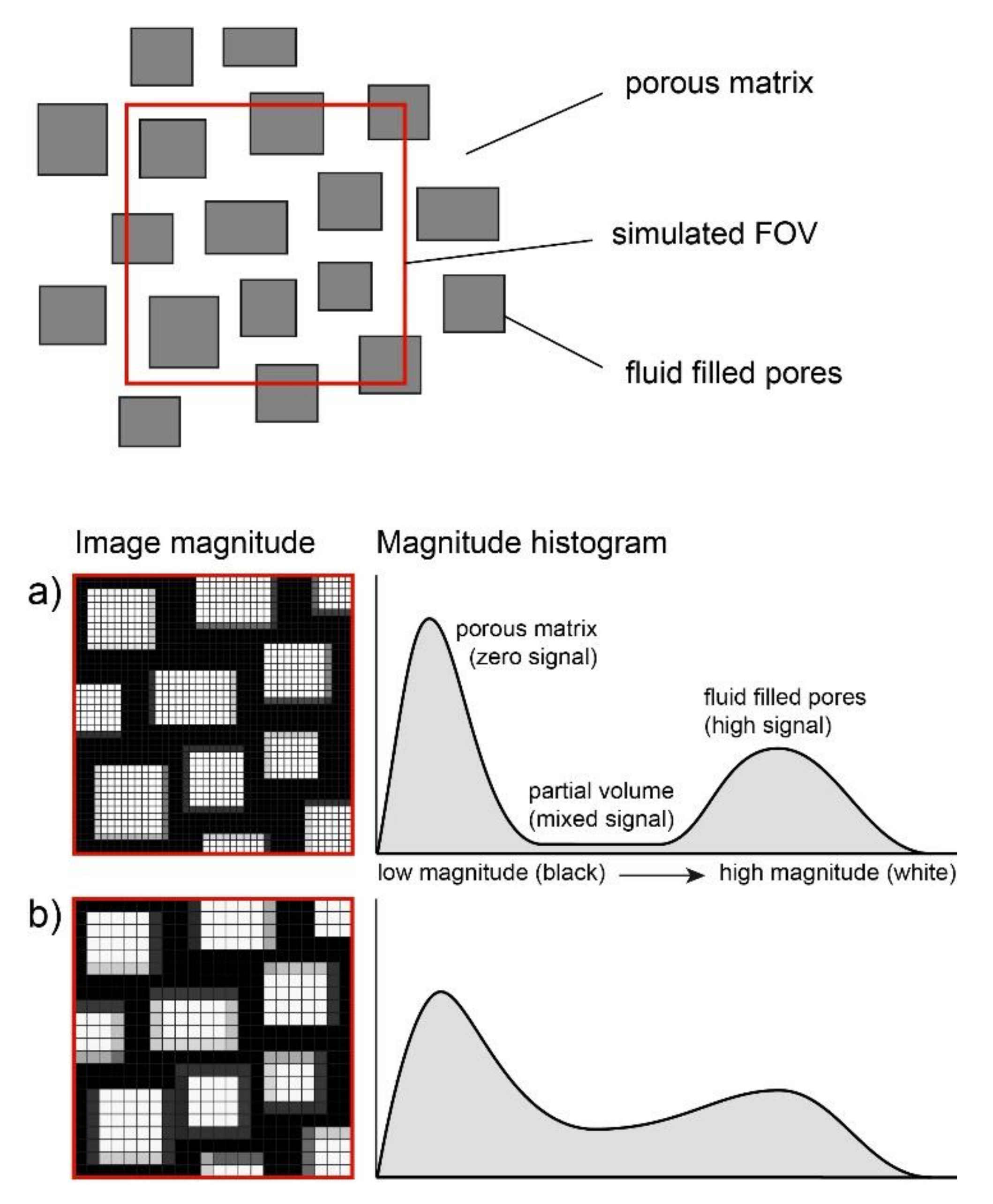
Fundamentals of the Data Reconstruction in MRV

With MRI and MRV, the data of the measured object are sampled in the spatial frequency domain, referred to as the k-space. After a Fourier transform of these data, the object is reconstructed in the image space on a uniformly spaced rectangular grid with up to three spatial dimensions.
The voxels in the image contain complex values. The magnitude values in the image depend on the parameters of the pulse sequence used for imaging, and on the physical properties of the measured object. In the event that the focus is on the velocity data and liquid distribution, the pulse sequence can be adjusted so that the magnitude values represent the local spin density. The hydrogen proton in water or other liquids is typically used as a signal source, and voxels containing these liquids have high magnitude values in these images. The surrounding structures that do not contain a signal-carrying liquid contain only rectified noise, which results in low magnitude values. Partial volume voxels that lie on the border between the two regions contain a mixed signal and, therefore, a medium magnitude value.
In velocity-encoded MRV measurements, each voxel in the fluid volume contains quantitative information relating to the fluid velocity. The phase angle value θ in each voxel is made proportional to the velocity via velocity-sensitive magnetic field gradients. With the parameter VENC (which describes the velocity sensitivity of the image phase angle), the velocity in each voxel can be reconstructed by the relation:
u = V E N C π θ .
Before an analysis of the fluid dynamics is possible, the fluid volume must be extracted from the image. The simplest method is to divide the image by a threshold value based on the magnitude. All voxels with a magnitude value that is larger than this threshold are assigned to the fluid volume. This process is called image segmentation.
In order to demonstrate the challenges faced during the segmentation process, Figure 1 shows the image magnitude from a simulated measurement of a porous matrix. The histogram of the magnitude shows two peaks, one representing the porous matrix and the other representing the fluid-filled pores. Between these two peaks lies a region with medium magnitude that belongs to the partial volume voxels.
With a voxel size much smaller than the porous structures, the fraction of partial volume voxels is relatively low and the high-signal region is clearly distinguishable from the low-signal region (see Figure 1a). Any threshold value that is within the partial volume range would sufficiently extract the fluid geometry. With a lower measurement resolution (a larger voxel size), a higher fraction of partial volume voxels is generated that fills the region between the two histogram peaks (see Figure 1b). In this case, an accurate segmentation of the image magnitude is not possible.
In summary, the accuracy of MRV measurements of porous media depends strongly on the voxel size. A large voxel size not only leads to the poor discretization of the velocity field, but also to an increase in the fraction of the voxels that are partial volume voxels (which complicates the extraction of the fluid geometry and may lead to additional systematic errors).

2. Materials and Methods

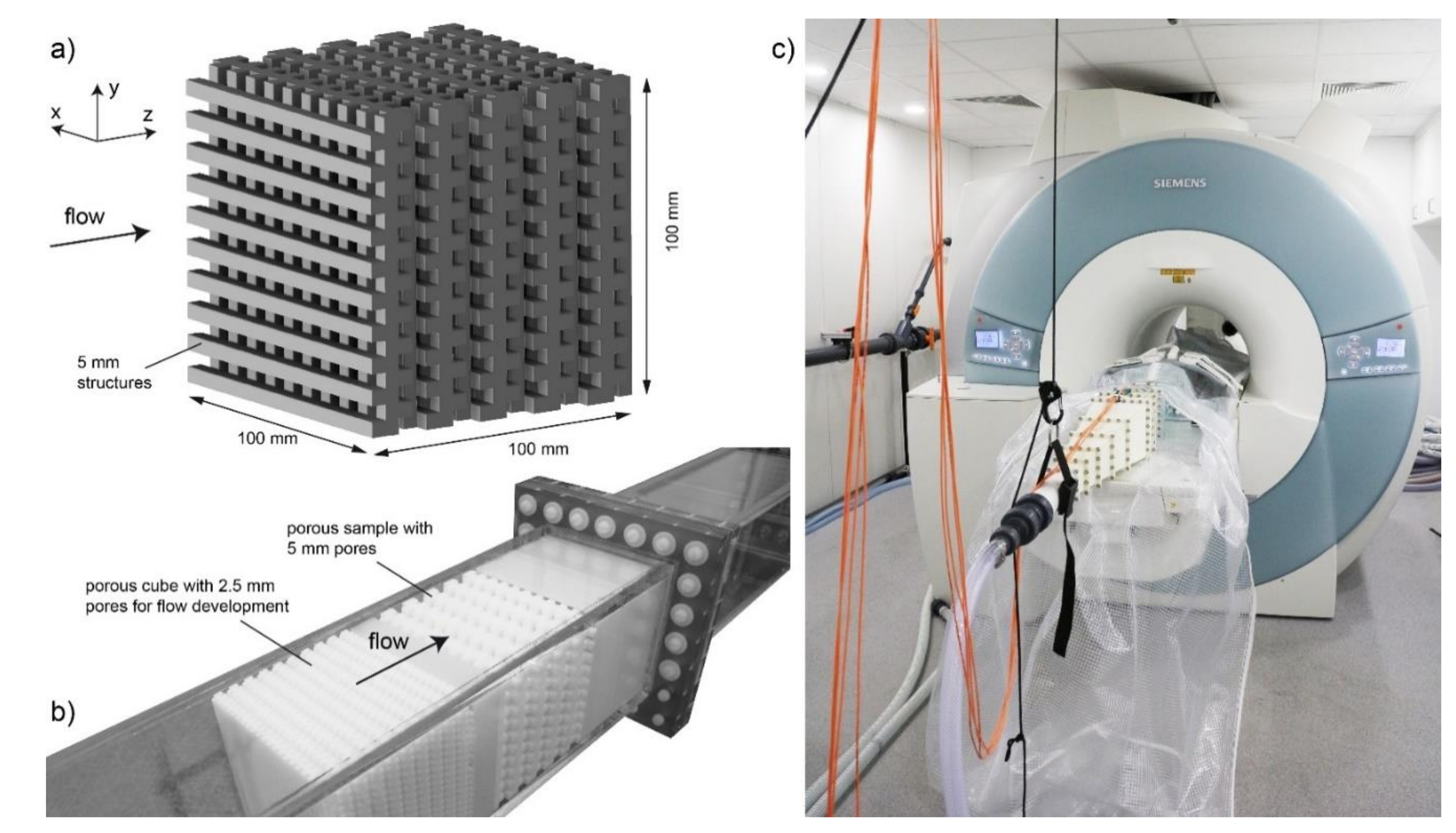
2.1. Experimental Setup

A regularly structured porous matrix is used to examine the measurement accuracy of MRV in porous media applications. The solid matrix is composed of distinct layers of uniformly distributed parallelepipeds, and these layers are “stacked” in the direction of the bulk flow (along the z coordinate direction) so that the longitudinal axis of each parallelepiped is (i) perpendicular to the direction of the bulk flow and (ii) oriented perpendicular to the longitudinal axes of the parallelepipeds of the adjacent layers. The parallelepipeds of alternating parallel layers are offset by a distance of one half of a pore’s thickness. This introduces tortuosity to the flow path. The periodicity and the orientation of the parallelepipeds is highlighted in Figure 2, in which the top panel corresponds to the x-z plane and the bottom panel corresponds to the same structure in the y-z plane. For more information on the model geometry, the reader is referred to [19].
In the MRV experiment, the porous matrix is built from parallelepipeds of 5.00 mm side lengths (so that the cross-sectional is 25.00 mm2), resulting in a characteristic uniform pore size of 5.00 mm. As shown in Figure 3a, the overall matrix is cubic with an edge length of 100 mm so that it is composed of 20 layers in the z-direction. In each layer, there are 10 bars oriented along the x- and y-directions. The matrix was fabricated with a polymer printer (Object30 prime, Stratasys, Rechovot, Israel) with a print deposition layer thickness of 16 µm.
As shown in Figure 3b, the matrix was placed inside a rectangular channel and held in place by thin spacers. A similarly structured cube with 2.5 mm large pores was placed upstream to provide the matrix with uniform inlet conditions. Additionally, in order to keep inlet and outlet disturbances at low levels, the channel was extended by more than 0.5 m upstream and downstream of the test section (more than 100 pore lengths). The working fluid was a mixture of 65% glycerol and 35% water, including 1 g/L CuSO4 that was added to reduce the magnetic relaxation time scales of the liquid. The fluid was pumped through the porous sample at a constant volumetric flow rate of 15 L/min and a constant temperature 17.6 °C. The measured kinematic viscosity at this temperate is 15.5× 10⁻⁶ m2/s.
While the entire porous cube (100 mm × 100 mm × 100 mm) was scanned, only the flow through the central pore region was analyzed. With a low Reynolds number for the flows through the porous media, the variations in velocity associated with the outer wall (edge effects), as well as inflow and outflow effects, are restricted to a few pore layers (see the discussion in chapter 1.5.3 of [4]). Thus, it is anticipated that the flow in the inner pore region is homogeneous and in a fully developed state.
The superficial (Darcy) velocity in the central (50 mm × 50 mm × 50 mm) core region was determined from the MRV data to be 0.02625 m/s. Using the Darcy velocity and the characteristic pore length of 5.00 mm, the characteristic Reynolds number of this experiment is Re = 8.56.

2.1.1. MRV Protocols

All MRV tests were carried out on a 3 Tesla MRI system (Magnetom TRIO, Siemens Healthineers, Erlangen, Germany) with a maximum gradient amplitude and slew rate of 40 mT/m and 200 T/m/s, respectively. Two standard multi-channel receive-only surface coils provided by the vendor were used. Figure 3c shows the channel inserted into the MRI machine.
The velocity field inside the porous matrix was generated with a custom velocity-encoded phase-contrast gradient-recalled echo (GRE) sequence that had a velocity sensitivity of VENC = 0.2 m/s. The encoding scheme proposed by [20] was applied to minimize the number of errors caused by flow displacement. For more information on the exact pulse sequence designs, the reader is referred to [21]. The FOV is cubic with an edge length of 107.5 mm covering the entire porous sample. The isotropic resolution was set to 0.42 mm, resulting in more than 16 million data points. The acquisition was repeated nine times and then averaged to increase the SNR. Background phase errors were compensated for by taking a reference measurement without flow velocity (flow off). The measurement parameters are provided in Table 1.

2.1.2. MRV Data Processing
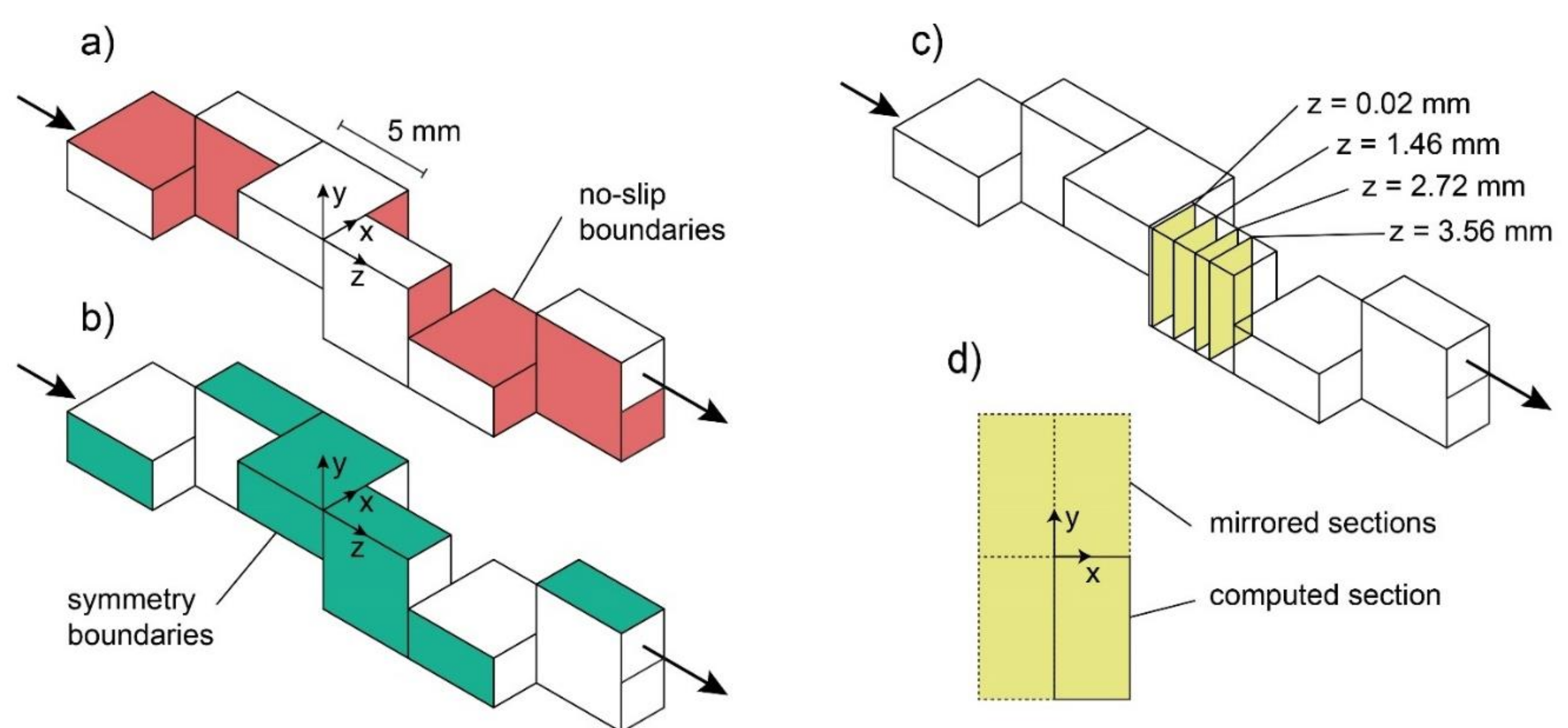
The image resolution is defined by the maximum absolute k-space coordinates in the raw data. If the k-space size is reduced by removing data points with high absolute k-space coordinates, the image size remains the same, but the voxel size increases. In a GRE sequence, as used here, each k-space data point is measured independently (neglecting the influence of noise correlations along the readout (RO) direction; see RO in Table 1). It can therefore be assumed that an image reconstructed from a subsequently reduced k-space is statistically the same as an image that was measured with reduced k-space.
The subsequent reduction of the k-space data in order to generate data sets with a lower resolution (larger voxel sizes) is a very useful technique. Only one high-resolution measurement needs to be carried out and all reconstructed images represent the same flow condition. All differences between these images can therefore be traced back to the voxel size.
Using this technique, 15 images were produced with an isotropic voxel size between 0.42 mm and 4.48 mm. Note that with the lowest resolution, the voxel size is only slightly smaller than the pore length scale of 5.00 mm.
The MRV image data were segmented to extract the fluid geometry. The image segmentation was carried out with the knowledge that the porosity is exactly ε = 0.50. The threshold value, which divides the image into the two regions, was set in such a way that exactly half of the voxels belong to the fluid volume, and thus the target porosity is achieved.

2.2. CFD Setup

A CFD study was carried out to measure the flow through a geometry that is representative of the porous media of the experiment. The CFD model uses the periodicity of the flow shown in Figure 2. Symmetry exists in the matrix structure and the anticipated flow (indicated by the dash-dot lines of Figure 2). Between these planes of symmetry, the flow paths through the medium may be individually represented by a single representative pore structure. This pathway through six layers of the medium is depicted in Figure 4. The same representative flow structures appear throughout the porous sample of the MRV experiments in Figure 3a.
While numerical simulations are not the focus of this study, this section provides some details of the numerical simulations that were conducted using the software package, Comsol version 5.5. The stationary “Laminar Flow” model of the “Single Phase Flow” model library is used to determine the solutions to the continuity and Navier–Stokes momentum equations with constant fluid properties. The fluid property values were chosen to be representative of those of the glycerol–water mixture of the experiment; the dynamic viscosity was assigned a value of 17.96 × 10⁻³ Pa s and the density a value of 1172 kg/m3.
The no-slip (zero velocity) boundary condition is imposed on all surfaces corresponding to the fluid–solid interfaces: on the fluid element, these correspond to all the internal faces and one half of the faces at the planes corresponding to the inlet and the outlet. An illustration of the faces of the element that are assigned the no-slip condition is depicted in Figure 4a. Symmetry boundary conditions are implemented on all surfaces corresponding to the planes of symmetry depicted by the dash-dot line of Figure 2. All the outer faces of the representative fluid element correspond to planes of symmetry; thus, the symmetry boundary condition (zero normal flux) is applied on all outer surfaces (depicted in Figure 4b by the green-shaded faces).
At the inlet pore structure, a uniform velocity of 0.105 m/s is specified, which corresponds to the Darcy velocity of the MRV experiment of 0.02625 m/s. The Reynolds number is the same as in the experiment and yields Re = 8.56. At the outlet of the pore structure, a uniform pressure of 0 Pa is imposed. A tetrahedral mesh was developed using the “normal” setting of the “physics-controlled mesh” with a minimum volume size of 0.1 mm and a maximum volume size of 0.335 mm, a growth factor of 1.15, and a curvature factor of 0.6; this resulted in a mesh composed of 179,646 elements.

3. Results and Discussion

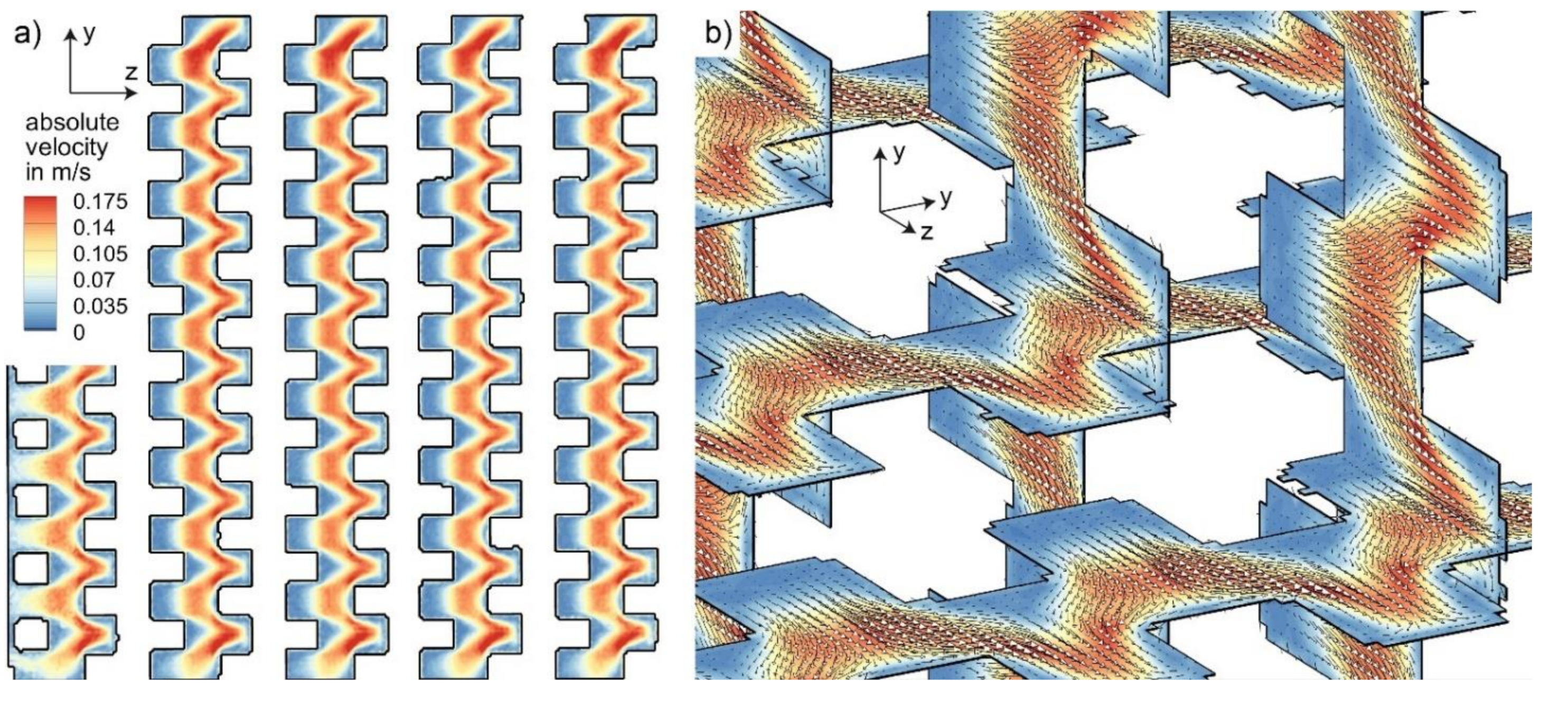
3.1. MRV Velocity Field

Figure 5 shows the absolute velocity field u x 2 + u y 2 + u z 2 1 / 2 inside the porous cube measured with the smallest voxel size of 0.42 mm. The data were segmented according to the method described in Section 2.1.2. Figure 5a shows that the flow is evenly distributed over the pores in the central core region. Edge effects at the channel walls are restricted to only one or two layers. Figure 5b provides another view of the data, demonstrating the quality of the measurement.
The measurement uncertainty for this data set was estimated with the difference method proposed in [22] and yields 0.0065 m/s. The uncertainty is 3.2% of the VENC value. Note that the uncertainty is lower for the data sets with larger voxels.

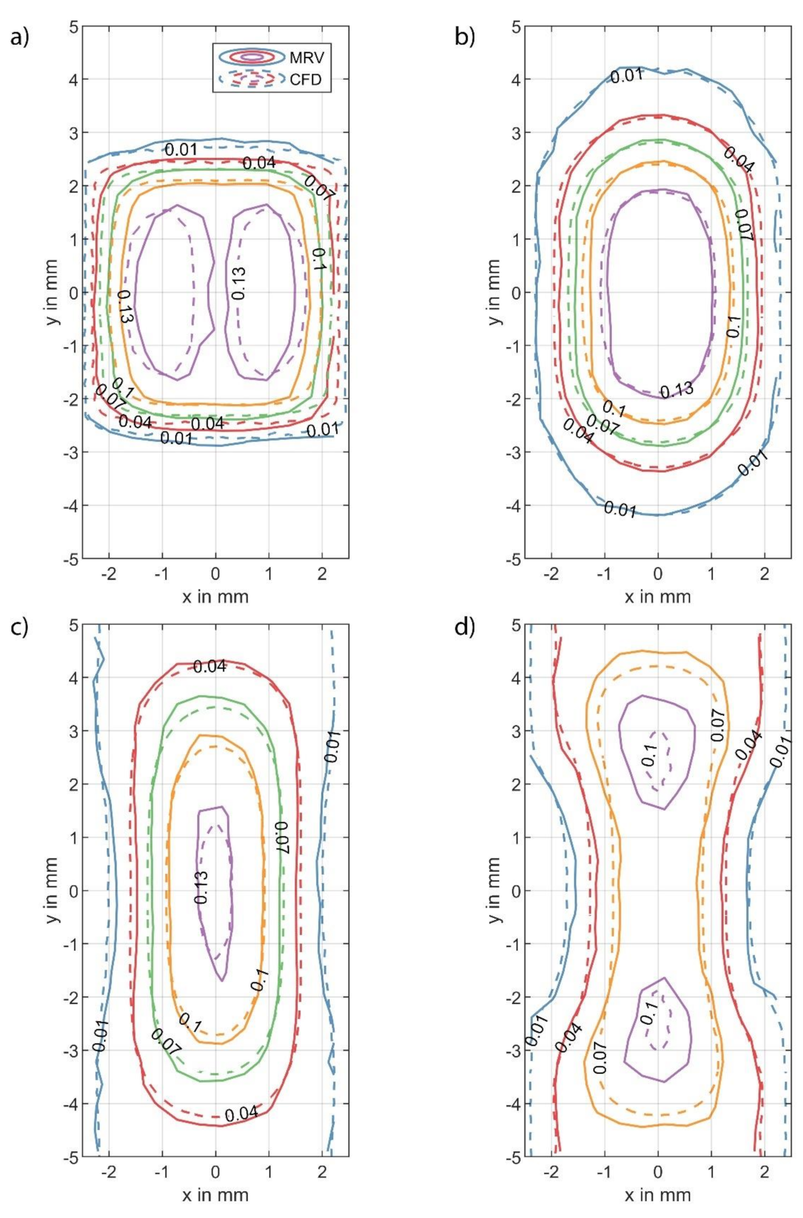
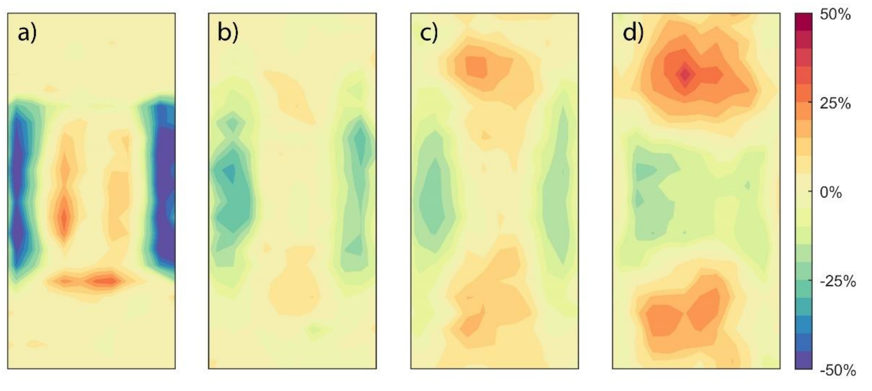
3.2. Comparison to CFD Results

The baseline accuracy of the MRV measurement was examined through a comparison with the CFD results. The MRV data taken from a single pore located within the core region were transformed onto the CFD-coordinate system specified in Figure 4. Experimental and simulation data were taken along planes that represent the same relative pore positions (see the relative planes of Figure 4c). These data were then processed onto the same grid in Matlab 2020b (The MathWorks, Inc., Natick, MA, USA) using the ScatteredInterpolant function. The comparison between CFD and MRV was conducted for the four planes depicted in Figure 4c, which correspond to the following distances from the inlet of the fourth pore layer: 0.02 mm, 1.46 mm, 2.72 mm, and 3.56 mm. The CFD data were mirrored across the symmetry boundaries, as shown in Figure 4d, to reconstruct a full cross-section of the fluid channel. Contours of the axial velocity component (uz) along these specified planes have been plotted in Figure 6 for the MRV results (solid lines) and for the CFD results (dashed lines).
In all cases, there is very good agreement between the MRV and the CFD data. Near the inlet (Figure 6a), both data sets show the double side-by-side core structure resulting from the symmetry of the porous medium. The lower velocity profiles are in better agreement, though even the position of the high-velocity profiles (0.13 m/s) are in qualitative good agreement, although the MRV contours are shifted slightly to the inside. Progressing into the pore (Figure 6b,c), the double core structures merge and the momentum spreads throughout the channel. At a location closer to the outlet of layer four, a transition to a vertically arranged double core structure is seen (Figure 6d). For the higher velocity values, the MRV contours are spread slightly further apart compared to the CFD data.
Figure 7 shows the difference in local velocity between the CFD and MRV data as a percentage of the volume average intrinsic velocity (0.0525 m/s). The same planes as in Figure 6 are processed. The highest difference is observed near the inlet in the regions with the highest velocity gradients (see Figure 6a and Figure 7a). The root-mean-square difference of all the depicted data is 12.4% of the volume-average intrinsic velocity.
Differences between the MRV and the CFD can be explained in part as follows. The MRV used a relatively large voxel size (0.42 mm) that was 8.4% of the pore length, so the MRV data distribution along any plane will clearly be distributed in a much coarser manner. Additionally, there are partial volume voxels at the walls that contain data for regions occupied by both fluid and solid. In spite of this, there is very good agreement between the experiment and the numerical predictions.

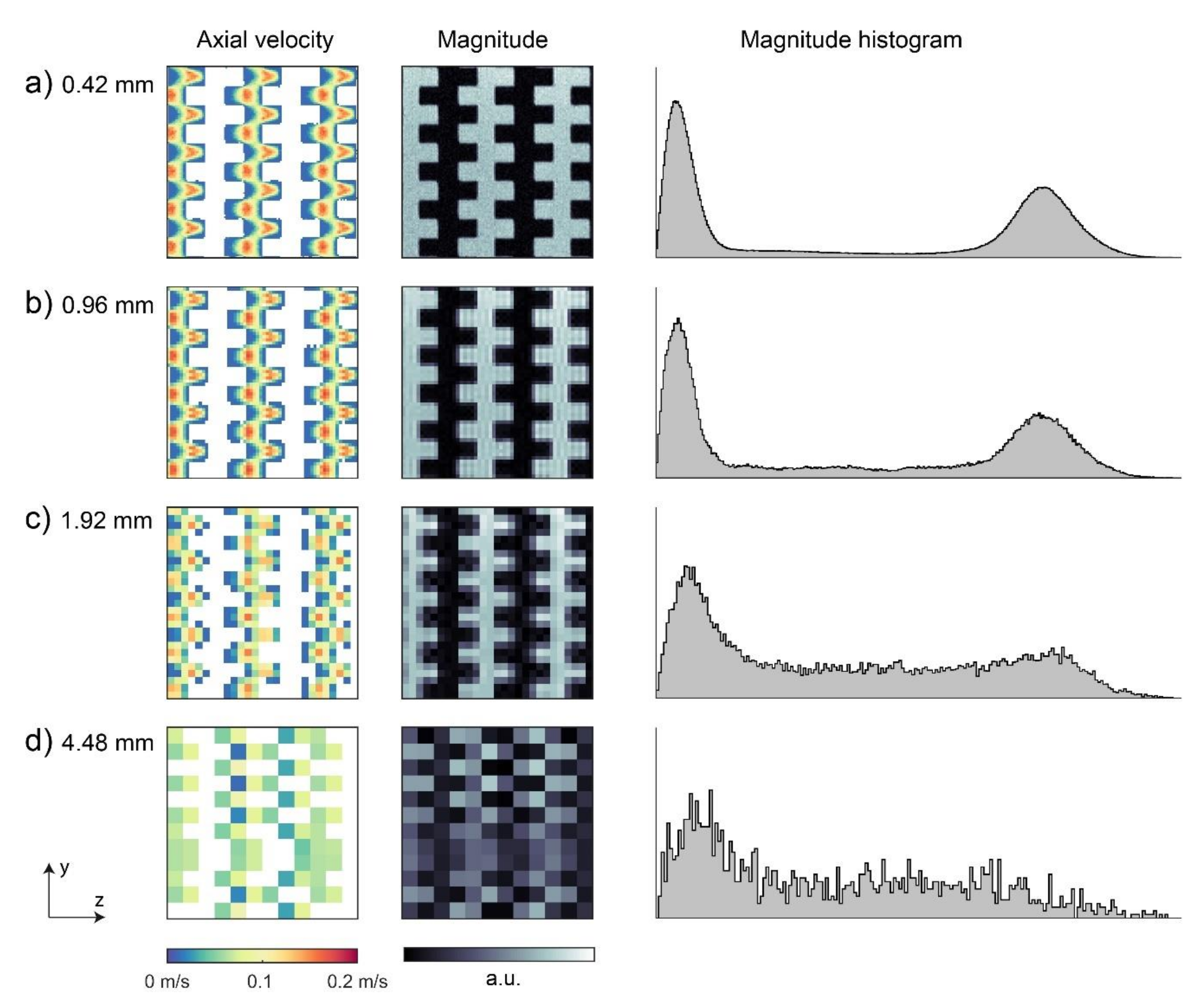
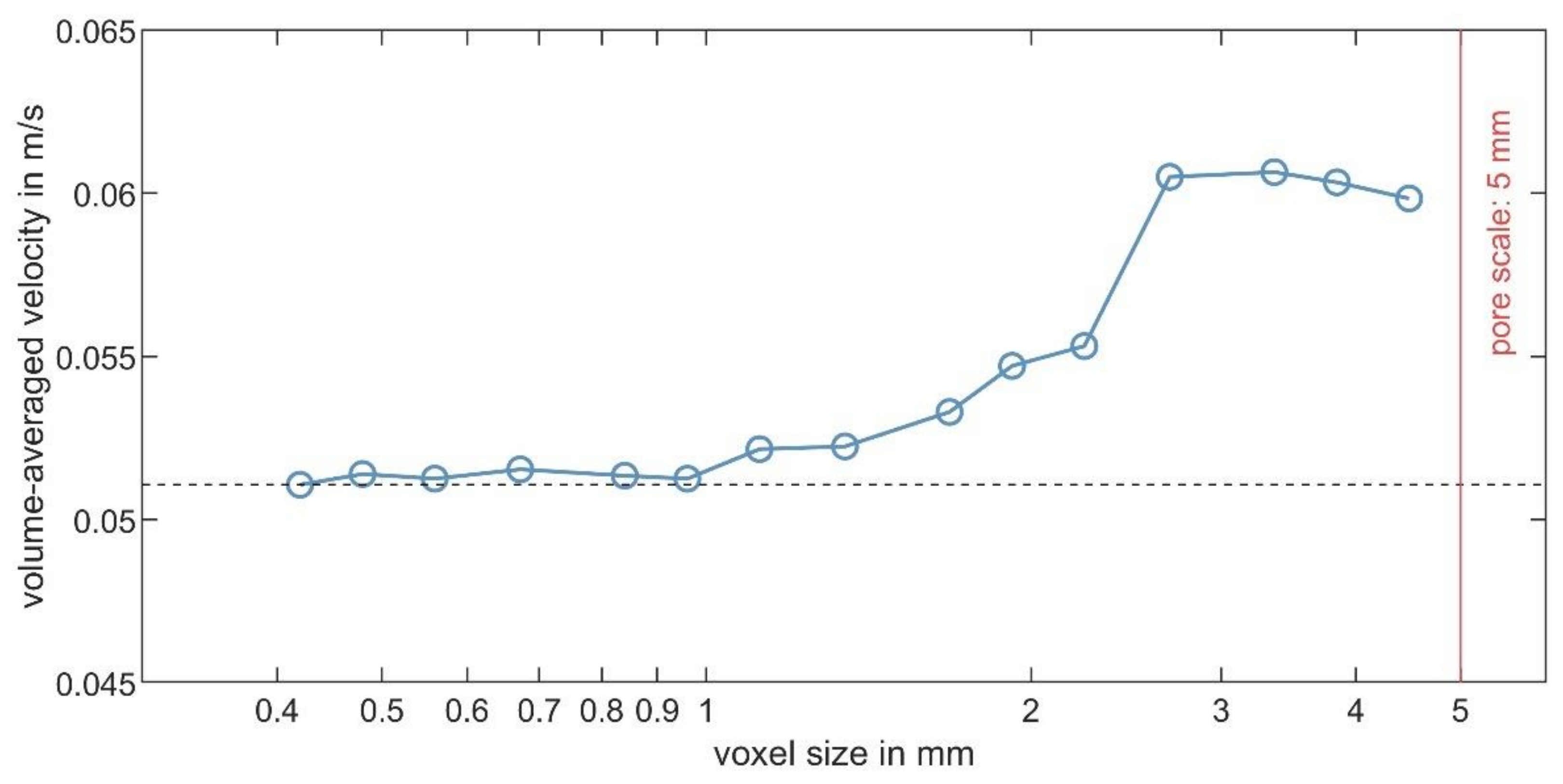
3.3. Study on Voxel Size

As described in Section 2.1.2, the MRV data were reconstructed with reduced k-space data to produce data sets with a lower resolution. The effect of different voxel sizes is shown in Figure 8. With a lower resolution, the porous structure and the velocity field became less well discretized until a segmentation of the pore network was no longer possible, as shown in Figure 8c,d. Additionally, the same qualitative trend as illustrated in Figure 1 can be observed in the depicted histograms: the relative number of partial volume voxels grows with increasing voxel size, which fills the histogram region between the two signal peaks.
From Figure 8, it can be summarized that the data quality gradually decreases with the lower resolutions. However, this analysis gives no indication of the minimum voxel size required. Therefore, we further investigated how the voxel size affects the data in terms of flow quantification and the local velocity distribution.

3.3.1. Influence of the Voxel Size on Flow Quantification

The volume-averaged velocity in the examined volume has a fixed value, since all data sets were computed from the same raw data. Consequently, any discrepancy in the volume-averaged velocity that occurs with a larger voxel size is an indication of an error. Using the velocity data from all 15 data sets, the volume-averaged velocity was computed with the axial velocity values (w) for the fluid volume:
1 N i = 1 N w i ,   w i t h   i   ε f l u i d   v o l u m e .
Figure 9 shows the results of Equation (2). It can be seen that with a voxel size below 1 mm, there is a plateau in which the volume-averaged velocity values stay constant. The maximum deviation in this region is only 0.09%. For voxels larger than 1 mm, the deviation increases substantially and reaches 18% for the largest investigated voxel size.
This analysis shows that a voxel size of up to 20% of the pore size is sufficient in this experiment. Within this range, a lower resolution only leads to a coarser representation of the velocity field but does not add systematic errors. With a voxel size of more than 20% of the pore size, additional systematic errors appear that make the data unusable for analyzing the volume-averaged flow.

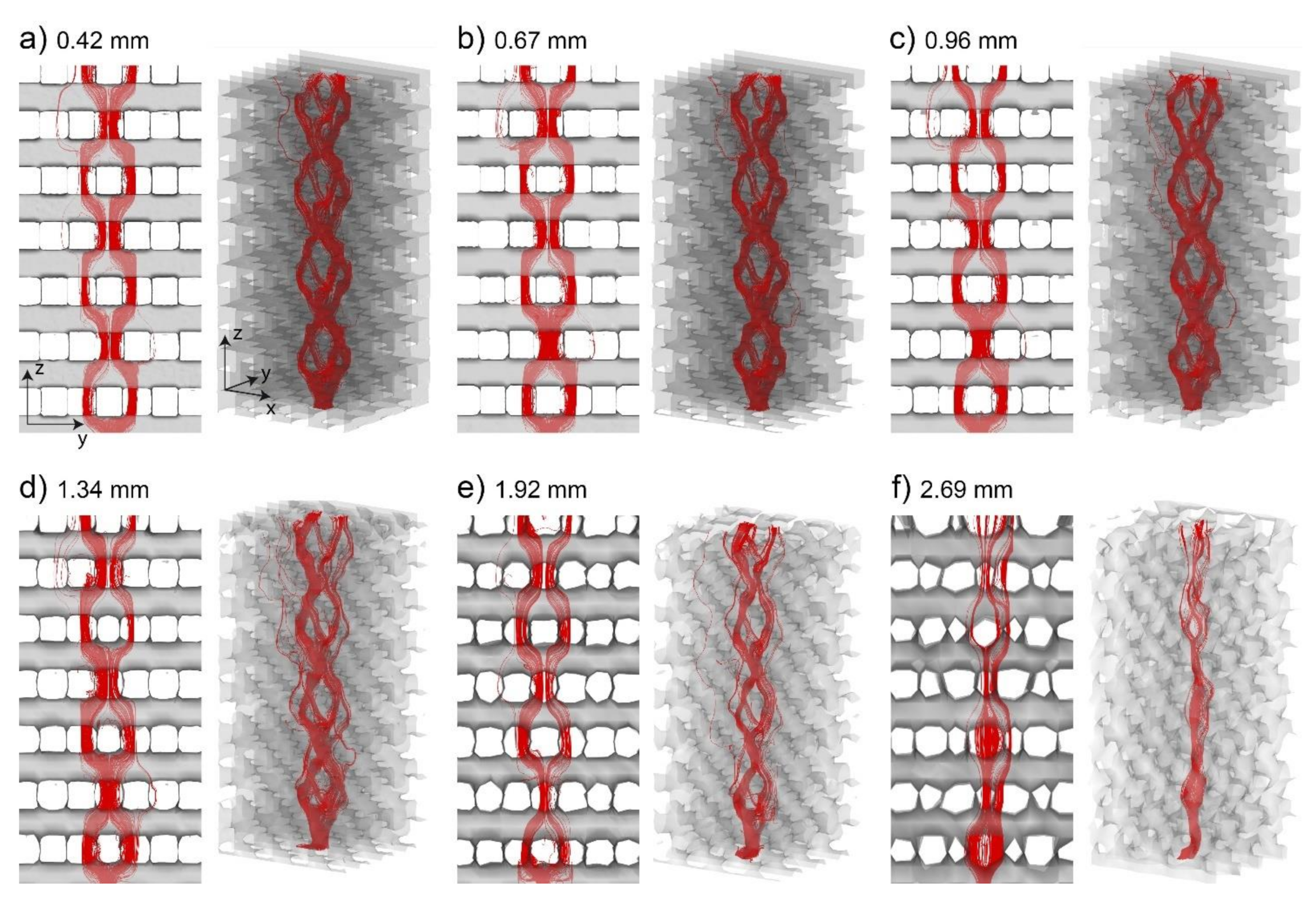
3.3.2. Influence of the Voxel Size on the Local Velocity Distribution

Next, an analysis was conducted to assess the influence of voxel size on the qualitative representation of the flow field. Similar to the study of Ref. [15], streamlines were calculated from the MRV data and tracked through the pore network. Using the post-processing software, Tecplot360 (Tecplot Inc., Bellevue, WA, USA), 300 streamlines were randomly seeded in a single sub-channel (5 mm × 5 mm) at the inlet plane. The seeding coordinates are the same for all data sets.
Figure 10 shows the streamline distribution for six selected voxel sizes. Figure 10a–c represents data with voxels smaller than 20% of the pore size. Almost exactly the same streamline distribution can be seen in these images, which confirms the results of the mean flow analysis in Section 3.3.1: a voxel size set at 20% of the pore size appears sufficient in this experiment.
The images in Figure 10 also include the 3-dimensional pore geometry as measured with the MRV. The depicted iso-surfaces represent the fluid surface, which was reconstructed from the MRV magnitude data as explained in Section 2.1.2. It can be seen that the edges of the reconstructed pore geometry are rounded off with larger voxels, but this does not seem to affect the streamline results in Figure 10a–c.
Figure 10d–f shows that the streamlines deviate for the larger investigated voxels. While a voxel with 1.34 mm length may still be sufficient to capture the qualitative flow behavior, strong deviations are visible with a voxel size of 1.92 mm and larger. Moreover, it can be seen that the measured pore geometry is highly distorted for the two largest depicted voxel sizes.

4. Conclusions

In this paper, MRV measurements are performed for the laminar flow of a 65% glycerol, 35% water mixture through a regularly periodic porous matrix made with a 3-dimensional polymer printer. The MRV data were compared to a laminar CFD analysis of the same flow. The experiment and the numerical prediction showed a good agreement in the local velocity field, which increases the confidence in the experimental approach.
The voxel size of the MRV data was systematically varied to examine the effect of the voxel size on the measurement accuracy. The aim was to find the largest possible voxel size that reveals the flow field sufficiently without adding significant errors.
A voxel size of less than 20% of the pore size was found to be sufficient if the data are used to determine volume-averaged properties, such as flow rate and mean velocities. A smaller voxel size would not improve the accuracy; instead, the smaller voxel size would unnecessarily increase the measurement effort. A similar trend was observed with the local velocity data. The calculated streamlines were unaffected by the voxel size for voxels smaller than 20% of the pore size. Based on the presented results, it can be concluded that a voxel size of up to 20% of the pore size can be sufficient in this type of experiment.
In summary, this study shows that even with a relatively low measurement resolution, data on quantitative 3-dimensional velocity fields can be obtained through porous flow systems with short measurement times and low measurement uncertainty. These results are useful for determining an appropriate voxel size for future MRV experiments.

Author Contributions

M.B. contributed all MRV-related work, S.F. ran the CFD simulations, S.B. was involved with the writing and early CFD work. The following breakdowns of roles are applicable to this paper: conceptualization, M.B. and S.B.; methodology, M.B. and S.B.; software, M.B., S.B. and S.F.; validation, M.B.; formal analysis, M.B.; writing—original draft preparation, M.B. and S.B.; writing—review and editing, M.B., S.B. and S.F.; visualization, M.B. and S.F.; supervision, M.B. and S.B. All authors have read and agreed to the published version of the manuscript.

Funding

This research received no external funding.

Data Availability Statement

The data presented in this study are available on request from the corresponding author.

Conflicts of Interest

The authors declare no conflict of interest.

References

  1. Vafai, K. (Ed.) Porous Media: Applications in Biological Systems and Biotechnology; CRC Press/Taylor & Francis Group: Boca Raton, FL, USA, 2010. [Google Scholar] [CrossRef]
  2. Vafai, K. (Ed.) Handbook of Porous Media; CRC Press/Taylor & Francis Group: Boca Raton, FL, USA, 2015. [Google Scholar] [CrossRef]
  3. Dullien, F.A.L. Porous Media: Fluid Transport and Pore Structure; Academic Press, Inc.: San Diego, CA, USA, 1992. [Google Scholar] [CrossRef]
  4. Nield, D.A.; Bejan, A. Convection in Porous Media; Springer: New York, NY, USA, 2013. [Google Scholar] [CrossRef]
  5. Northrup, M.A.; Kulp, T.J.; Angel, S.M. Fluorescent particle image velocimetry: Application to flow measurement in refractive index-matched porous media. Appl. Opt. 1991, 30, 3034–3040. [Google Scholar] [CrossRef] [PubMed]
  6. Saleh, S.; Thovert, J.F.; Adler, P.M. Measurement of two-dimensional velocity fields in porous media by particle image displacement velocimetry. Exp. Fluids 1992, 12, 210–212. [Google Scholar] [CrossRef]
  7. Gladden, L.F.; Mitchell, J. Measuring adsorption, diffusion and flow in chemical engineering: Applications of magnetic resonance to porous media. New J. Phys. 2011, 13, 035001. [Google Scholar] [CrossRef]
  8. Kutsovsky, Y.E.; Scriven, L.E.; Davis, H.T.; Hammer, B.E. NMR imaging of velocity profiles and velocity distributions in bead packs. Phys. Fluids 1996, 8, 863–871. [Google Scholar] [CrossRef]
  9. Manz, B.; Alexander, P.; Gladden, L.F. Correlations between dispersion and structure in porous media probed by nuclear magnetic resonance. Phys. Fluids 1999, 11, 259–267. [Google Scholar] [CrossRef]
  10. Ogawa, K.; Matsuka, T.; Hirai, S.; Okazaki, K. Three-dimensional velocity measurement of complex interstitial flows through water-saturated porous media by the tagging method in the MRI technique. Meas. Sci. Technol. 2001, 12, 172–180. [Google Scholar] [CrossRef]
  11. Sankey, M.; Holland, D.; Sederman, A.; Gladden, L. Magnetic resonance velocity imaging of liquid and gas two-phase flow in packed beds. J. Magn. Reson. 2009, 196, 142–148. [Google Scholar] [CrossRef] [PubMed]
  12. Wu, A.-X.; Liu, C.; Yin, S.-H.; Xue, Z.-L.; Chen, X. Pore structure and liquid flow velocity distribution in water-saturated porous media probed by MRI. Trans. Nonferrous Met. Soc. China 2016, 26, 1403–1409. [Google Scholar] [CrossRef]
  13. Lovreglio, P.; Das, S.; Buist, K.A.; Peters, E.A.J.F.; Pel, L.; Kuipers, H. Experimental and numerical investigation of structure and hydrodynamics in packed beds of spherical particles. AIChE J. 2018, 64, 1896–1907. [Google Scholar] [CrossRef]
  14. Romanenko, K.; Xiao, D.; Balcom, B.J. Velocity field measurements in sedimentary rock cores by magnetization prepared 3D SPRITE. J. Magn. Reson. 2012, 223, 120–128. [Google Scholar] [CrossRef] [PubMed]
  15. Onstad, A.J.; Elkins, C.J.; Medina, F.; Wicker, R.B.; Eaton, J.K. Full-field measurements of flow through a scaled metal foam replica. Exp. Fluids 2011, 50, 1571–1585. [Google Scholar] [CrossRef]
  16. Sadeghi, M.; Mirdrikvand, M.; Pesch, G.R.; Dreher, W.; Thöming, J. Full-field analysis of gas flow within open-cell foams: Comparison of micro-computed tomography-based CFD simulations with experimental magnetic resonance flow mapping data. Exp. Fluids 2020, 61, 124. [Google Scholar] [CrossRef]
  17. Yang, X.; Scheibe, T.D.; Richmond, M.; Perkins, W.A.; Vogt, S.; Codd, S.L.; Seymour, J.; McKinley, M.I. Direct numerical simulation of pore-scale flow in a bead pack: Comparison with magnetic resonance imaging observations. Adv. Water Resour. 2013, 54, 228–241. [Google Scholar] [CrossRef] [Green Version]
  18. Meinicke, S.; Möller, C.-O.; Dietrich, B.; Schlüter, M.; Wetzel, T. Experimental and numerical investigation of single-phase hydrodynamics in glass sponges by means of combined µPIV measurements and CFD simulation. Chem. Eng. Sci. 2017, 160, 131–143. [Google Scholar] [CrossRef]
  19. Munro, B.; Becker, S.; Uth, M.F.; Preußer, N.; Herwig, H. Fabrication and Characterization of Deformable Porous Matrices with Controlled Pore Characteristics. Transp. Porous Med. 2015, 107, 79–94. [Google Scholar] [CrossRef]
  20. Nishimura, D.G.; Jackson, J.I.; Pauly, J.M. On the nature and reduction of the displacement artifact in flow images. Magn. Reson. Med. 1991, 22, 481–492. [Google Scholar] [CrossRef]
  21. Schmidt, S.; Flassbeck, S.; Bachert, P.; Ladd, M.E.; Schmitter, S. Velocity encoding and velocity compensation for multi-spoke RF excitation. Magn. Reson. Imaging 2020, 66, 69–85. [Google Scholar] [CrossRef] [PubMed]
  22. Bruschewski, M.; Freudenhammer, D.; Buchenberg, W.B.; Schiffer, H.-P.; Grundmann, S. Estimation of the measurement uncertainty in magnetic resonance velocimetry based on statistical models. Exp. Fluids 2016, 57, 83. [Google Scholar] [CrossRef]
Figure 1. The effect of the voxel size on the distribution of the image magnitude illustrated with a simulated measurement of a porous sample with (a) high resolution and (b) low resolution. ’’FOV’’ stands for “field of view”.
Physics 03 00079 g001
Figure 2. Side views of the layered porous structure in the x-z and y-z planes with dash-dot lines indicating planes of symmetry. Note that the planes of symmetry bisect the pores in lateral directions. In this figure, the parallelepipeds are alternately colored blue and red to indicate the same layers in the two views.
Physics 03 00079 g002
Figure 3. Description of the verification experiment: (a) porous sample with staggered grid similar to [19], (b) assembly of the flow channel, (c) photo taken during MRV measurement.
Physics 03 00079 g003
Figure 4. The geometry and boundary condition locations of the CFD model. Red faces in (a) denote no-slip boundaries. Green faces in (b) denote symmetry boundaries. The yellow planes in (c) show the data that are compared with the MRV data and the origin of the z-axis, which is placed relative to the interface between layers three and four. These planes are mirrored as shown in (d) to reconstruct the full-sized channel.
Physics 03 00079 g004
Figure 5. Velocity field obtained with the highest resolution of 0.42 mm: (a) selected slice; (b) 3-dimensional view including velocity vectors.
Physics 03 00079 g005
Figure 6. Comparison of the MRV (solid lines) and CFD (dashed lines) axial velocity component (uz) contours along planes in the fourth layer of the pore structure as depicted in Figure 4 at the following distance from the inlet of layer four: 0.02 mm (a), 1.46 mm (b), 2.72 mm (c), and 3.56 mm (d).
Physics 03 00079 g006
Figure 7. Local differences in the data from Figure 6. Depicted is the axial velocity from MRV minus the axial velocity from CFD divided by the average intrinsic velocity (0.0525 m/s) at the following distance from the inlet of layer four: 0.02 mm (a), 1.46 mm (b), 2.72 mm (c), and 3.56 mm (d).
Physics 03 00079 g007
Figure 8. Velocity field for voxel sizes of 0.42 mm (a), 0.96 mm (b), 1.92 mm (c), and 4.48 mm (d) shown for: axial velocity (uz) in a selected (50 mm × 50 mm) slice (left column), magnitude data used for image segmentation (middle column), and magnitude histograms of the central (50 mm × 50 mm × 50 mm) volume of the porous cube (right column).
Physics 03 00079 g008
Figure 9. Volume-averaged velocity in the fluid-filled space as a function of the voxel size.
Physics 03 00079 g009
Figure 10. Streamlines calculated from the MRV data for voxel sizes of 0.42 mm (a), 0.67 mm (b), 0.96 mm (c), 1.34 mm (d), 1.92 mm (e), and 2.69 mm (f), each representing a view of the y-z plane (left panels) and in an isometric view (right panels). The depicted flow geometry represents the fluid boundaries which were reconstructed from the MRV magnitude by applying a threshold.
Physics 03 00079 g010
Table 1. Description of the sequence parameters.
No. of Voxels (x,y,z)Voxel Size
(mm)
Encoding
Direction
TE
(ms)
TR
(ms)
Flip Angle (°)BW (Hz/pixel)VENC (m/s)AveragesTotal Time (h)
256 × 256 × 2560.42 × 0.42 × 0.42RO PE SS5.18.6204070.296
RO: readout direction; PE: phase encoding direction; SS: slab selection direction; TE: echo time; TR: repetition time; VENC: describes the velocity sensitivity of the image phase angle; BW: bandwidth.
Publisher’s Note: MDPI stays neutral with regard to jurisdictional claims in published maps and institutional affiliations.

