1. Introduction
Data exfiltration is a common cyberattack in which information is removed, stolen, or copied from a computer without prior authorization or approval. There have been several high-profile cases of data exfiltration attacks, such as the 2017 Equifax data breach, in which the personal identifiable information (PII) of 143 million Americans was exfiltrated through an Apache Struts exploit [
1]. Information such as credit card numbers, Social Security numbers, birthdays, passwords, addresses, and financial records are all examples of PII held in systems that, if not adequately protected, are at risk of being attacked and compromised. The cost of the global data exfiltration protection market is estimated to reach USD 99.3 billion by 2024, according to some reports [
2].
Studies have demonstrated that such attacks are detectable using network anomaly detection techniques [
3,
4,
5,
6,
7,
8,
9,
10]. Few of these use graph approaches as a way to better inform detection models [
11]. Most approaches focus on global characteristics as features used in detection models than the nature of links and associated traffic between devices in a network [
6] (i.e., local characteristics). In our past work, we have demonstrated that network topology and associated local characteristics between devices can be incorporated in statistical models for graphs that then can be used in such a manner to detect DNS exfiltration attacks [
11].
The approach used past week information to predict daily anomalies in DNS traffic. However, DNS exfiltration is unique in the effect that it has on network traffic. It can be detected heuristically because the size of each DNS request is limited to about 253 bytes [
12] and, as such, large data exfiltrations will create large amounts of DNS requests. This is different from more “regular” traffic such as HTTP where volumes of data can be transferred via a single TCP connection or through multiple connections. This paper aims to expand the previous body of work by demonstrating the efficacy of such a technique on data exfiltration over (a) HTTP traffic and (b) hourly baselines. The latter further highlights that the technique can be fine-tuned reliably in various time windows depending on the context and traffic that is utilized in.
The contributions of this approach build upon our past work [
11] and are as follows:
The method utilizes topology information based on the graph representation of network traffic to summarize a network’s structural properties and to use such information in the statistical detection of an anomaly. This is different from detecting anomalies using global network indicators such as single node or whole network gigabytes of traffic. We achieve this by using exponential random graph models.
The method requires netflow data that are already collected as a common security practice in the industry.
The method aims to be an intuitive alert indicator that analyst can use to triangulate information about potential anomalies in the network.
The method can be configured to detect anomalies in various types of traffic and over variable time windows that can be used as baselines for network anomalies. In particular, an hourly time window allows for a much quicker incident response compared to daily time windows.
The rest of the paper is organized as follows. In
Section 2, we outline related work in the field of network anomaly detection related to our method.
Section 3 describes our proposed method from processing packet capture data to running graph models and the time series analysis used for anomaly detection.
Section 4 describes the experimental design, delving into finer detail on the configuration of the different components, as well as our data collection process and experimental procedure that focuses on HTTP traffic over hourly intervals.
Section 5 provides a statistical analysis and interpretation of our experimental results, as well as details the computational requirements of our method.
Section 6 discusses known and expected limitations of this method. Finally,
Section 7 provides some suggestions for future research in this particular domain.
2. Related Works
We organize the section below based on thematic units related to anomaly detection as it is approached through various lenses.
2.1. Anomaly Detection and Exfiltration
Exfiltration countermeasures can be placed into three categories: preventative, detective, and investigative [
13]. Under the detective category, there are further subtypes, such as host-based, network-based, and content-based detection. Our proposed framework falls under the host and network-based anomaly detective countermeasure category, as we are using both host data (ports), as well as network data (total flow). For example, a study used a Multivariate Anomaly Detection with Generative Adversarial Networks (MAD-GAN), consisting of Long Short-Term Memory (LSTM) Generator and Discriminator components to learn multivariate time series data from cyber–physical Systems (CPSs) [
14]. One application example for this is CPU usage. Test data were then evaluated on an anomaly score, based on discrimination and reconstruction. Another study used an Isolation Forest machine learning model to enhance existing DNS exfiltration detection approaches by incorporating both high-throughput tunneling and low-throughput malware detection into their solution [
15]. The one-class classifier Isolation Forest model was trained on DNS logs, which periodically extract features such as character entropy and longest meaningful word. Similar to the study that used the MAD-GAN architecture, an anomaly score was given for each sample and if it exceeded a certain anomaly threshold, an alert was raised.
2.2. Time Series Methods for Anomaly Detection
Time series approaches for network anomaly detection also exist. For example, a study used Attention Mechanism-CNN-LSTMs for time series analysis and anomaly detection of Industrial IoT (IIOT) network data, such as edge device failure detection [
16]. The authors noted that existing Deep Anomaly Detection (DAD) solutions could not be directly applied to IIOT with distributed edge devices due to privacy concerns and inflexibility. A Federated Learning (FL) technique was instead used in which the training algorithm was distributed across decentralized edge devices holding local data samples. The AMCNN attention mechanism was highlighted as a means to improve focus on important features in the time series, as well as aid in feature extraction. Another study also focused on time-series-analysis-based anomaly detection, suggesting an Exponential Weighted Moving Average (EWMA) model, or CNN-based time series analysis to learn filters capturing repeating patterns in the time series, which is treated as a one-dimensional image [
17]. Further creative approaches to time series detection also exist. A study contributed a novel time series detection approach called Series2Graph based on first representing time series subsequences as vectors and embedding them into a vector space [
18]. In the vector space, overlapping trajectories correspond to recurrent patterns in the time series data, and a graph can be constructed in such a way that nodes are based on intersecting trajectories and whose edges are based on transitions among subsequences. The graph model encodes the normal behavior of the time series and allows for differentiating between frequently occurring patterns and anomalous behavior in time series data.
2.3. Other Methods for Anomaly Detection
Techniques beyond supervised learning and time series analysis have also been used. For example, a study explored the usage of k-means clustering algorithms in the detection of anomalous and potentially malicious host connections in a network [
19]. Specifically, a clustering engine was used to create clusters based on extracted feature sets, which include source bytes per packet, producer consumer ratio, and number of peers and unique source ports. An elbow method selected the number of predefined clusters, and connections were scored. Then, anomaly alerts were raised based on Euclidean, Minkowski, or Manhattan distance measures. A similar study avoided direct packet analysis, noting the disadvantages in terms of computational cost and privacy and focused on anomaly detection using tensor rank decomposition (PARAFAC) [
20]. The study collected upload/download byte and packet counter data from home routers of an ISP and processed that data into tensors, which could then be decomposed. The Random Forest classifier was then used for anomaly detection on the extracted residuals from the tensor rank decomposition.
2.4. Patents for Anomaly Detection
Existing patents and patent applications can also be found in the literature. A patent introduced a real-time anomaly detection method that used a Latent Dirichlet Allocation (LDA) model to analyze groups of annotated time series data [
21]. A locality-sensitive hashing function or algorithm determines the number of anomalous groups across the time series data, and this parameter was inputted into the LDA. Another patent introduced a throttling bucket system which limits the rate at which service requests can be fulfilled by a server. The throttle bucket has an associated bucket level, which indicates the amount of service requests that can be fulfilled before restrictions are put into place [
22]. Every service request is assigned a cost, associated with its amount, complexity, credentials, and its requested data’s sensitivity. Exfiltration attempts and another malicious attacks would theoretically drain the bucket such that the system is shut down to prevent further attacks.
2.5. Our Method’s Proposition
The aforementioned approaches demonstrate the feasibility of anomaly detection based on various techniques including time series analysis. However, the use of graphs for anomaly detection poses difficulties as well as opportunities. The strength of our method compared to all these related studies lies in the utilization of node labels and terms, the ability to analyze multiple protocols, as well as the hourly analysis employed by our approach. Labeling nodes allow for a more fine-tuned graph analysis, and our method is flexible, potentially allowing for multiple protocol traffic patterns to be considered in anomaly detection.
3. Proposed Method
Our proposed method is a three-step process. It was originally described in a past work for daily anomaly detection on DNS data, and we have adapted it for the purposes of analyzing other types of data (e.g., HTTP traffic) within shorter timeframes [
11].
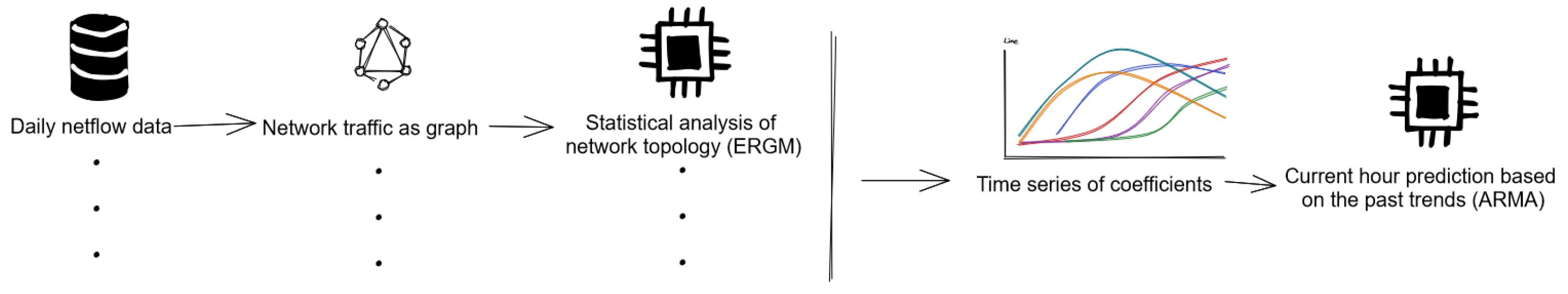
We first process PCAP data hour-by-hour into netflow files. This step is described in
Section 3.1. Using each netflow file, we represent each network-hour as a graph with nodes and valued edges and run a graph-based machine learning model known as an Exponential Random Graph Model (ERGM) to produce a log-odds coefficient. This produces an hourly snapshot of network features as coefficients. The ERGM is further discussed in
Section 3.2. Autoregressive Moving Average (ARMA) is trained on most of the data (aside from reserved testing data), and for the remaining few hours, it gives a prediction window for each hour representing what it expects to be a range of non-anomalous coefficient values. If our observed data point falls outside the prediction window, ARMA considers this anomalous. The prediction window is of a variable size and can be adjusted easily to optimize detection. ARMA is discussed in more detail in
Section 3.3.
3.1. Processing PCAP Data into Netflow
Packet Captures (PCAP) (dataset or real-time traffic) is processed on a per-packet basis where we extract information of interest such as source IP address, destination IP address, source port, destination port, and number of bytes from each packet. We then aggregate packets over a predefined time period (our study focused on hourly) and output a netflow file for each time period, indicating the sum total of bytes transferred between each pair of nodes. During the packet aggregation process, we can customize our processing to filter packets based on protocol such as HTTP or NTP (identified via the port that is used in a packet or some other method, e.g., payload analysis). We discuss details on the specific dataset that was used for experimental purposes for this paper further in
Section 4.1.
The netflow files are then further analyzed and annotated to classify nodes into server or host (i.e., client). This classification was based on the ports that each IP address is using, as the identity of utilized ports usually reveals if a device is a server or host. For example, an IP address only using port 80 is potentially a web server, whereas an IP address using ports between 50,000 and 60,000 as a source is usually deemed to be a host. This information aids in the statistical analysis of network topology, as some ERGM terms specifically analyze bipartite networks. The method is shown on
Figure 1.
3.2. Statistical Analysis of Network Topology
Traditionally, ERGM have been used by social scientists to analyze social networks for the presence of certain network substructures, such as connections, mutual connections, triads, and cliques, and how social mechanisms may influence their formation. The incorporation of randomness allows the model to account for the fact that the observed network being inputted, with its valued edges and nodes, is just one possibility among a set of potential networks with the same nodes. This is because there is an underlying stochastic process that affects the frequency of certain manifestations. By attempting to deduce the parameters that influence these stochastic processes, we can then estimate a probabilistic measure, the log-odds coefficient, that indicates how usual or unusual the observed network is based on certain features.
ERGM is a subset of the exponential family of functions [
23]. The exponential family of functions is a set of probability distributions defined over some measure
such that the probability distribution density relative to
can be expressed in the following form:
The exponential family contains many commonly used probability distributions, such as the normal distribution, and Bernoulli distribution. The defining characteristic that makes exponential family functions so useful is that they can model an arbitrary amount of independent identically distributed data, which are needed in modeling network graph edges whose behaviors are similar but may be independent of each other. An ERGM is defined as follows:
where
Y is a random network with the same number of vertices as
y, our input network.
is a vector of sufficient statistic dependent on the input network
y, and
is a vector of model parameters associated with
. A statistic is defined as sufficient when its origin sample gives no additional info about the population source compared to the statistic itself. Lastly,
is a normalizing constant that can be expanded to
The expanded form of the ERGM equation is therefore
Due to the exponentially increasing computational requirements associated with increasing graph sizes, it would be infeasible to compute and analyze every possible set of graphs for a set of nodes in order to deduce the true log-odds coefficient of an observed graph. Instead, ERGMs utilize Markov Chain Monte Carlo Maximum Likelihood Estimation (MCMC-MLE) to estimate the log-odds of the input graph’s structure by simulating a random graph distribution using a Markov chain, comparing the distribution to the input graph, adjusting the parameter values, and repeating this process until the parameter estimates converge. The Markov chain is assumed to have a similar equilibrium behavior to the probability distribution in question. The model runs the Markov chain in order to generate a sample which can then be used for estimation.
The log-odds coefficients are associated with certain user-defined terms, such as dyadic connections, k-star, triangular connections, and the likelihood of their appearance in the graph. Other terms measure values of edges, such as the
term, which measures probability of finding edges with a value greater than
x. By utilizing different terms in an analysis, we can have a more cohesive understanding of network traffic. A discussion into the specific terms that we used in this study can be found in
Section 4.3. In the end, the topological awareness of the ERGM translates to a comprehensive understanding of network traffic behavior. We would like to further note a parallel between traditional frequentist statistical methods (e.g., regression) and ERGM. In ERGM, the dependent variable is the network, while the independent variables are the local network properties that we test for.
3.3. Time Series Analysis of Coefficients
A time series is a sequence of chronologically ordered data, of which there are two varieties: discrete-time and continuous-time. Discrete-time indicates that data are collected in equally spaced time intervals (every hour, every day), whereas continuous-time indicates that data are collected non-stop. The motivation behind performing a time series analysis varies by field and by project. For example, in economics and meteorology the primary motivation is forecasting, whereas in machine learning and data mining, time series analysis can serve as a tool for anomaly detection, classification, and clustering.
Our method utilizes the Autoregression Moving Average (ARMA) model [
24] for the purpose of anomaly detection on the ERGM time series data. The ARMA model was chosen because it excels at modeling weakly stationary stochastic processes, such as network traffic data, which exhibits daily as well as weekly patterns. The ARMA model consists of two polynomials: an AR (autoregression) polynomial and an MA (moving average) polynomial. The autoregression polynomial can be expressed as follows:
where
c is a constant,
is a white noise random variable, and
are parameters. An AR model by itself forecasts future data points in a time series data set by learning the Partial Autocorrelation Function (PACF) for an order of
p points, where
p is a parameter representing the number of lagged values the PACF includes and the order of the AR model. For example, an order 8 AR model’s prediction for point
would depend on the values of
to
and their respective learned coefficients
. This notation is usually represented as AR(8).
The Moving Average portion of the model can be expressed as follows:
where
is the mean of the time series,
are error terms,
q is the order of the MA model, and
are model parameters. The error term
for some point at index
i is calculated as follows:
where
is the actual value and
is the predicted value. The error terms as a whole are assumed to be normally distributed with a mean of zero and are sometimes referred to as white noise error terms. The MA model makes predictions on future data points by tweaking its parameters according to the error in previous predictions.
Combined, these two components make up the ARMA model. The notation ARMA(
p,
q), therefore, refers to the following model:
In our approach, the ARMA is trained first; then. it calculates variable-sized prediction windows for a few points into the future; and if the observations fall outside the range, an alert is raised for an anomalous event. The anomaly detection technique is further described in
Section 4.4.
4. Experimental Design
We evaluated our proposed method by designing and running experiments with real-world PCAP data and injecting the subsequent netflow files with three sizes of exfiltration attempts: 5%, 10%, and 25% traffic increases. The subsequent HTTP netflow files were analyzed with the ERGM model. HTTP is only one among many application layer protocols in use, and we ultimately decided on HTTP because of its commonality, and its frequency of use in modern computer networks. It is also substantially different from previous DNS traffic examined using this technique, since HTTP has a large variance in bytes per packet [
11].
The experimental design has five sections.
Section 4.1 discusses our data set selection process and criterion for evaluating quality.
Section 4.2 details the exfiltration scenarios and how they were injected into our training data.
Section 4.3 goes over the ERGM specific configuration, and the terms we used to describe the behavior of the network.
Section 4.4 discusses the ARMA specific configuration, including the anomaly detection windows and the preprocessing for stationarity. Finally,
Section 4.5 discusses our experimental trial configuration.
4.1. Data Procurement
In the real world, there is a reasonable upper bound to the size of computer networks, as universities, corporations, and other organizations usually do not exceed the sixth order of magnitude (hundreds of thousands) in terms of membership. Therefore, the ideal packet capture dataset should originate from a network with at least a few hundred hosts (or servers) in order to minimize the effects of noise caused by individual hosts. In addition, the data should be anomaly-free so as to allow ARMA to learn the baseline behavior of the network. In terms of length, it is recommended that ARMA is trained with at least 50 but ideally over 100 contiguous data points in order to effectively learn a time series’ behavior [
25]. Since in this study, we performed an hourly analysis of a network, this translated to at least 2 days of packet capture network data.
After an extensive search through PCAP repositories and libraries, we selected the University of New Brunswick’s ISCX 2012 Intrusion Detection Evaluation Data Set [
26] for our experiments. It features seven complete labeled days of PCAP data from a large network. However, four out of seven days of data were known to contain anomalies, such as HTTP Denial of Service and internal infiltration, and therefore, we decided to drop these four days and to juxtapose the three anomaly-free days for our experiments in order to establish are clean baseline. The three anomaly free days were Friday (11 June), Saturday (12 June), and Wednesday (16 June). We treated the Wednesday data as if it were the weekday before the Friday data. This gave us a 72 h anomaly free data set that was nearly continuous and had two weekdays and one weekend.
We processed PCAP data into netflow files, filtering by protocol and writing a new netflow every hour in a new data set. This resulted in 72 netflow files that were subsequently analyzed in order to aggregate ports used by IP addresses and then label each node as either “host” or “server”. In the case of HTTP, the presence of port 80 indicated a server. The approach can be easily updated for different protocol labeling requirements (including HTTPS). It is important to note that filtering by protocol substantially reduces the amount of data traffic, as well as nodes, in netflow files. Filtering by HTTP, our netflows averaged around 20 nodes, with 2 HTTP server devices apparent, and the rest labeled as “hosts”.
After labeling hosts, we condensed the netflow files further into “edge hour” files, which represents the network in edge list form, aggregating by source ip, destination ip, and bytes transferred, disregarding the port identities.
4.2. Exfiltration Scenarios
Our three main exfiltration scenarios were 5%, 10%, and 25% increases in a particular edge’s traffic in the netflow file. Further, we ran three testing scenarios: exfiltration in a single hour, exfiltration over several continuous hours, and exfiltration over random hours. The selection of hours to be injected with exfiltration was randomized. In the case of exfiltration over several continuous hours and in the case of exfiltration over random hours, the number of hours to be injected was also randomized. We also randomized the selection of the injected edge within the “edge hour” file.
4.3. ERGM Configuration
Once exfiltration was injected into certain “edge hour” files, we used ERGM to flatten the “edge hour” files into a time series. As previously discussed, the ERGM is a probabilistic model that uses MCMC-MLE, and as such, repeated executions on the same dataset could yield a range of results. Therefore, repeated trials are necessary in order to ensure a fair representation of the distribution. Burnin refers to the number of proposals before MCMC begins sampling, and this parameter should be set relatively high to ensure convergence, at least around 50,000. We also set the sample size and interval to 5000 and found that this was a reasonable balance of execution time and precision after a few test runs. ERGM’s max iterations parameter was set to around 200, to allow for convergence. Since we are using valued ERGM analysis (
ergm-count package [
23]) as opposed to binary ERGM analysis, the trust region parameter for MCMC-MLE was set to at least 1000, and the reference mode parameter should be set to geometric in order to model valued edges.
There are nearly a hundred terms available in the ergm package, and each one of them has its own requirements and limitations. The network object we created from the “edge hour” data was valued; directed; and as such, requires valued ERGM analysis. Even though the vertices in our network were labeled either host or server, the bipartite mode was not compatible with our analysis, as our network is not bipartite in the strictest sense. This is because inter-host and inter-server communication is possible. Therefore, we eliminated bipartite, undirected, and binary-only terms and selected from the approximately remaining thirty terms through a process of trial and error, as not every term produced meaningful results for our data set. This is because an absence of certain local features for ERGMs makes it impossible to obtain a consistent log-odds coefficient result for a term. In the end, we selected the
sum and
nodecov terms. The sum term does not depend on labeling and focuses on how “natural” a particular weighted edge is in the graph. On the other hand, nodecov incorporates the label information in its analysis and determines how likely communication is between hosts, servers, or in between. We postulated there is more detection potential with terms such as nodecov, which incorporate attribute labels like server and host into their algorithm, and the results discussed in
Section 5 support this postulation. Finally, we verified the plots for all these coefficients in order to ensure that the sampled distributions by the MCMC were normal.
4.4. ARMA Configuration
A time series is considered stationary if its mean and variance are constant over time. Since stationarity is an underlying assumption for the ARMA model, the coefficients outputted from ERGM must be adjusted to ensure stationarity. This is especially advisable when a small sample size is used, in which any significant amount of noise or outliers could cause the time series to appear to violate stationarity. Therefore, to ensure stationarity on the ERGM outputs, a technique of rolling z-score subtraction was used, where the average of the previous 7-h z-score was subtracted from the present term to a produce more stationary time series data. In order to confirm the stationarity of the transformed time series, our ARMA model contains an optional stationarity report method, which runs an Augmented Dickey Fuller unit root test on the transformed data. Although, the details of unit roots and the Augmented Dickey Fuller unit root test are beyond the scope of this paper, in simple terms, unit roots are trends in stochastic processes that indicate the process is unpredictable. Therefore, if such trends exist in data then the data should not be used for time series analysis, as it may cause spurious regressions and erratic behavior in t-scores and z-scores. Unit root tests, such as the Augmented Dickey Fuller, are one such tool that is used to detect such unit roots.
Once stationarity for our data was confirmed, we used the pmdarima package in our ARMA model to perform hyperparameter tuning and to determine the optimal order p and q for ARMA. As a side note, pmdarima is usually used to fit ARMA(p,q).
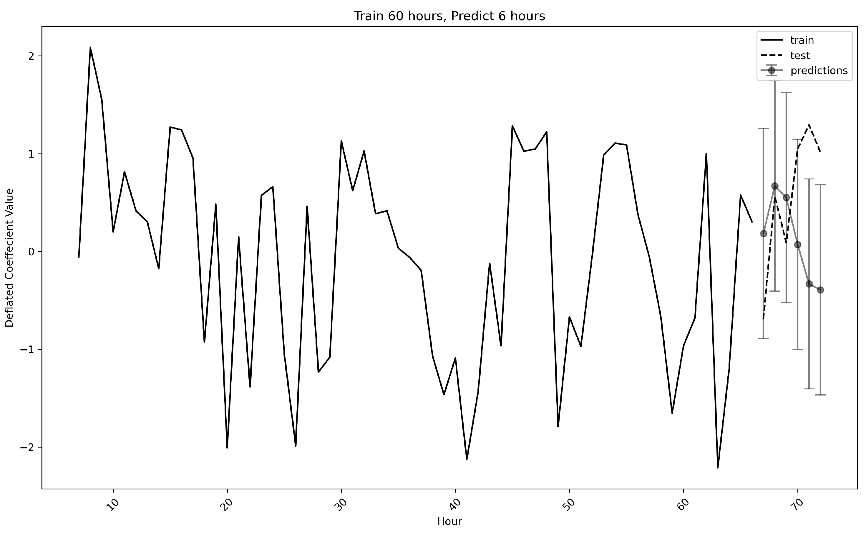
The train–test splitting is an important factor to consider with ARMA. The test set size should be kept small, as ARMA’s predictive ability decreases in accuracy as time goes on from the start of the prediction period. For our experiments, we decided to train on the initial 66 h and to predict on the terminal 6 h.
Figure 2 shows a sample ARMA output trained on ERGM coefficients for 66 h of data and a prediction on a test set of 6 h. Predictions come in the form of windows which are based off the standard deviation of the ERGM coefficients. The size of the windows can be varied in our proposed solution, allowing for a higher threshold (e.g., one standard deviation) for high traffic days, and a lower threshold (e.g., 1/4 standard deviation) for low traffic days. For our experiments, we chose window sizes of 1/4, 1/2, and 1 standard deviations. If an observed data point falls outside its prediction window, it is labeled as anomalous.
4.5. Experimental Procedure
Our experimental procedure was designed as follows. We had three exfiltration sizes, three detection window sizes, and three injection modes. The sizes were 5%, 10%, and 25% of additional traffic. The injection modes were single hour, multiple hour, and random hour. Finally, the three detection windows sizes were 1/4, 1/2, and 1 standard deviation. The entire training process was separated by term and by protocol. Since we used two terms, we produced two ERGM baseline time series, two trained ARMA models and two sets of injected network data that were used with their respective protocol ARMA model.
We conducted 100 trials for each exfiltration size and exfiltration mode setting, reusing “edge hours” between differing detection window sizes. This gave us 900 trials per detection window size and a total of 2700 trials per term. In total, we conducted 5400 trials. The accuracy of ARMA in predicting exfiltration for each trial was recorded, and the results are discussed in
Section 5.
5. Results
5.1. Performance
We evaluated the experimental performance using four metrics: precision, recall, accuracy, and F2 score. These metrics were calculated using binary classification data from ARMA, the implementation of which was added into the ARMA script. Precision is a measure of positive predictive value. In our case, it represented the proportion of ARMA flagged hours that were actually anomalous. Recall is a measure of sensitivity and indicated the proportion of anomalous hours that were correctly identified by ARMA. Accuracy indicated the proportion of correctly predicted hours, normal and anomalous combined. Finally, F score takes into account both recall and precision into a harmonic mean. Its related function, the F2 score, gives two times more consideration to recall than precision. We preferred F2 score because in the field of anomaly detection, it is more important to actually flag anomalous hours. In other words, the sensitivity of the model must be appropriate. Often times, precision alone does not provide a clue as to the overall sensitivity of the model.
Table 1 demonstrates the ARMA performance on the sum term, whereas
Table 2 shows the performance on the nodecov term. Some cells are empty due to division by zero. ARMA is known to have decreasing predictive ability as the test set increases in size. ARMA predicted the first four hours of the baseline time series test set correctly, and the terminal two hours incorrectly, so we thus decided to split the data analysis, considering the test set’s first three hours’ and last three hours’ performance separately. The last three hours’ performance can be considered statistically irrelevant due to poor baseline performance. Precision was positively correlated with the threshold window size for all three modes, which was expected since as the model’s range of normal values increased, there were less false positives. On the other hand, recall is inversely correlated with the ARMA threshold across all terms and modes, since a smaller threshold is more selective about which hours are normal, resulting in more false and true positives. In the single injection mode, accuracy was positively correlated with threshold, but this was due to the fact that most hours were already normal, and there was only a single anomalous hour. In the other modes, accuracy was either consistent across window sizes or slightly inversely correlated. F2 scores were inversely correlated with threshold size, since recall was also inversely correlated with threshold size. The sum and nodecov term do appear to have some discrepancy in their descriptive power. Nodecov performed much better than sum in multiple injection mode, while performing about equally in single and random mode. In summary, the reduced performance of nodecov could be attributed to multiple factors, but it is likely that due to the use of the HTTP protocol across multiple devices, the effect of this statistic in detecting anomalies is slightly suppressed.
Overall, the findings indicate that there is value in labeling devices and incorporating such labels in the analysis of communication between the in graphs. Regardless of the injection mode or threshold, node covariance appeared to surpass the summative metric based on the weight of edges. This makes intuitive sense since an increase in particular traffic link over two devices may appear to be significant; however, knowing what is the role of these devices increases the contextual understanding of an event. For example, a server would rarely communicate as devices with one another, yet a host communicating with a server is a much more likely event. Changes in either of these communication channels can have a different significance.
5.2. Comparison to Other Methods
As with our previous work, our method compares to other methods in terms of accuracy and computational overhead [
11]. A comparison is shown on
Table 3. These comparisons are not intended to be exhaustive but rather serve as representative examples of the choices available. As there are differences in the parameters and experiments outlined for these methods, ranges or averages are provided for the purpose of comparison. Consequently, although we present a wide range of accuracy for our method, in practice, most implementations will fine-tune the parameters to align more closely with the lower end of the range.
Moreover, the computational burden is influenced by the choice of algorithm, with certain techniques, like clustering approaches, being notably more resource-intensive. Models that necessitate training before making predictions, including our own method, often incur significant costs during the training phase but exhibit faster performance when identifying anomalies in a testing dataset.
Table 3 further illustrates the variation in computational overhead, which is attributed to the number of nodes considered in each approach. Graph-based methods face feasibility challenges when dealing with networks that have numerous nodes, whereas other supervised models can handle such scenarios due to the inherent structure of data points in those methods. Therefore, when assessing the practicality of implementing an anomaly detection technique, the size of the network becomes a crucial factor that affects the computational demands.
5.3. Computational Requirements
The computational requirements for this method were considerable. On an Intel Core i5-1035G4 @ 1.10 GHz, producing a single netflow file for a network hour required about an hour of computational time. With 72 network hours in our dataset, nearly a week was devoted to the process of creating netflow files for ERGM. In addition, the size of a PCAP file could also be limiting along with PCAP files that contain aberrant or corrupt packets. We used SplitCap to split our daylong PCAP files into hour-long tidbits in order to parallelize the processing.
The ERGM calculations took about 5 min per network hour, but a larger network would require exponentially more time. Past research that utilized ERGM in anomaly detection has indicated as much [
11]. ARMA computational requirements are also rather low, producing most of the predictions within a few minutes for hundreds of experiments.
6. Limitations
This method is limited by the computational time and space needed. PCAP files for large networks over a single day are usually at least 10–20 gigabytes in size, and producing the netflow for such a daylong PCAP can be a challenge. However, modern monitoring solutions already incorporate netflow collection at sensors (e.g., Suricata IDS can also collect netflow information).
ERGM calculations, especially MCMCMLE iterations, are extremely time-consuming, often requiring 20 min per iteration. Therefore, it is advisable to have access to computational resources before this method can be used on a real-time scale for a large network.
In addition, the availability and difficulty in procuring high-quality “normal” data can limit the effectiveness of the method. Ideally, this method would be trained on a week-long continuous anomaly-free sample of packets from a large organization’s computer network. In our study, we were limited to using a PCAP file as our baseline for producing hour normal hourly traffic baseline.
The ARMA model is limited in its temporal applicability, losing predictive power after just a few hours in the test set. This suggests any viable future model might need continuous new data every few hours to produce an up-to-date time series for ARMA. In other words, a real-time solution that aims at hourly anomaly detection should be fed with hourly up-to-date data. The ARMA model could also be potentially paired with a model with longer memory, such as an LSTM, which also specializes in analyzing time series data.
Finally, a 5%, 10%, or even 25% data injection on a network with several thousand nodes might prove to be too insignificant for the ERGM model to produce an anomalous coefficient for certain terms which do not take into account network geometry. Larger size networks should also be tested to establish the efficacy of such a method.
7. Future Work
There is considerable research potential in different anomaly detection frameworks. Future work will focus on applying other machine learning models besides ARMA/ARIMA to the time series data produced by the ERGM, such as and LSTM, EWMA (Exponential Weighted Moving Average) or other deep learning solutions, like CNN or RNN. Other protocols, such as HTTPS, SMTP, FTP or SSH could be analyzed for their traffic patterns and compared to HTTP. An anomaly detection system could potentially utilize our ERGM-ARMA system with input across several protocols and ERGM terms, aggregating their signals for anomaly detection. Future work could also focus on optimizing the run-time of the entire method by experimenting with multithreaded programming, parallelization, or cloud computing options. There is also an opportunity to eliminate the ARMA component by attempting to perform a temporal exponential random graph model. The computational overhead and feasibility of temporal ERGM would have to be evaluated.
In the more immediate term, it may be worthwhile to invest in PCAP data generation techniques or alternative data sources, since it is difficult to find reliable PCAP data. A future project might generate its own PCAP data simulating a network with several hundred hosts and servers, as opposed to the real-world limited size closed network we examined. This may result in a model that is easily adaptable to real-world network monitoring tasks for organizational entities with thousands of hosts. Additional terms in the ERGM library could also be evaluated for their descriptive power, such as nodecovar, nodeicov, and b1star.
8. Conclusions
Data exfiltration is a major cybersecurity issue which presents many complex challenges in detecting it. Our method is an effective approach to detecting data exfiltration on a network by analyzing its hourly PCAP traffic with exponential random graph models and using time series analysis tools, such as ARMA, to identify anomalies and as such potentially malicious exfiltration attempts. The performance of ERGM shows evidence of improving upon the incorporation of node label data, such as server and host, with the nodecov term. ARMA performance quickly declines after three or four hours of predictions, and works best with the 0.25 and 0.5 threshold settings. Future research will experiment with other time series detection models, as we continue to search for ways to effectively identify anomalous network behavior.


