1. Introduction
Surface waters, either permanent or temporary, with their distinct characteristics as rivers, lakes, reservoirs, and wetlands, are extremely dynamic entities that change over time and influence the hydrological water cycle. Depending on the prevailing hydrological conditions, the interactions between surface and subsurface water systems can make it rather complicated to delineate water recharge in karst terrains [
1,
2,
3,
4,
5]. In cases of landscapes that periodically fill with water, as topographic depressions in karst regimes, they may be subjected to flooding depending on prolonged rainfall and in some cases lateral flow from adjacent catchments discharging onto the lowland karst [
6,
7]. Excess recharge that cannot be accommodated by a karst aquifer due to insufficient aquifer storage or flow capacity can cause groundwater levels to rise and inundate basins as well as the surrounding areas [
7,
8]. This ephemeral flooding can pose significant risks to humans, farmland, and infrastructures [
9,
10,
11].
While the spatial distribution of surface water bodies on a global scale is adequately available [
12,
13,
14,
15,
16], the actual information on the location and extent of temporary water bodies is incomplete. Despite individual limitations, existing geospatial databases are valuable sources of information for all geographic latitudes due to satellite remote sensing (RS) advances that provide global coverage with a high spatial resolution.
Remote sensing measurements can provide valuable information on hydrological systems by mapping permanent or temporary water bodies and by providing the temporal and spatial variations in the water coverage. Satellite observations are an effective way to detect surface water over large areas with a short revisiting time, supporting operational monitoring and being a rapid as well as effective response to natural disasters, such as floods [
17,
18,
19,
20,
21].
Earth observation data from both optical and radar sensors offer the opportunity to map and monitor the spatiotemporal changes in water cover. Data from Copernicus Sentinel-1 (S-1) and Sentinel-2 (S-2) missions can provide significant monitoring capabilities for surface water detection and mapping. Sentinel-1 radar data have been widely used for water mapping [
22,
23,
24,
25,
26], since radar sensors have the advantage of operating in nearly all-weather/day–night conditions, overcoming the limitations of optical imagery. Most available algorithms typically focus on single-image techniques and change detection approaches [
27,
28], while others exploit large data stacks to delineate surface water [
22,
29,
30]. Radar backscatter is often used to distinguish water from surrounding areas, since strong specular reflection occurs at its surface, meaning that it appears to be very dark in radar images. For this purpose, among various techniques, thresholding approaches have been explored in cases of large datasets [
31,
32,
33,
34].
Water mapping by radar imagery can also be associated with additional remote sensing data, specifically multispectral optical imagery, for detecting the extent and evolution of water. Sentinel-2 optical data offer a high spatial resolution (10–20 m) with a nominal revisit time of 5 days, as well as monitoring in the near- and middle-infrared bands on a global scale [
35,
36,
37]. Since water shows a very low reflectance value in these ranges of the spectrum, water indices [
38,
39,
40,
41] are widely used to identify water surfaces. In addition to radar and optical imageries, soil moisture ocean salinity (SMOS) data can be used in advance to provide timely estimates of soil moisture every three days, with an accuracy of 4% at a spatial resolution of 50 km [
42]. Seasonal changes in soil moisture content are also important for contributing to the forecasting of hazardous events, such as floods [
43,
44,
45,
46].
Motivated by the need to improve existing global geodatabases of inland water bodies by fusing only remotely sensed data, as well as to build surface water data records for smaller and/or temporary water bodies linked to flooding phenomena in karst regimes, this paper aims (a) to compare multiple imagery sources to map and monitor, for the first time, the spatiotemporal changes in the ephemeral lakes in Chalkida that led to temporary inundations, (b) evaluate, with statistical analyses, the temporal and spatial dynamics of water storage using long-term remote sensing observations, and (c) create a water variations database that can serve as an important source of information for future water resource regulations in this region. The ultimate goal of this study is to create a framework for satellite-based water surface monitoring that will, in turn, provide important information to local authorities for hydrologic analyses and flood forecasting applications.
2. Hydrogeological Setting—Flooding Events
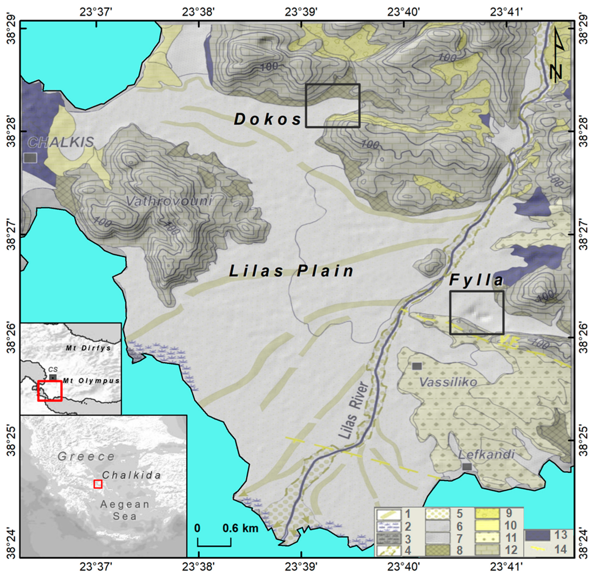
The municipality of Chalkida was selected as a pilot case for this study as it presents a representative example of temporary lake flooding in karst environments in proximity to river systems. Chalkida is located in the south of Evia, with its main geomorphological structures being the Dirfys Mt., reaching an elevation summit of 1743 m, and the Lilas River, with a drainage basin–fan delta system of about 300 km
2 flowing into the South Evoikos Gulf (
Figure 1).
The morphology of the area varies between the high relief of the NE as well as east mountainous zones (Mt. Dirfys and Mt. Olympus) and the low relief to the SW, where the Lilas River fan delta is located, a low plain area that was shown to be a shallow marine environment during Holocene [
47]. Several river channels have been activated in this area during severe rainfalls towards the south and west coastlines, causing the progradation of the Lilas River fan delta [
47] (
Figure 1). Although the climate conditions within the drainage basin show relatively high mean annual precipitation, on 11–12 September 2009 a severe flash flood event occurred and approximately 350 mm of rainfall was recorded in 28 h. The event resulted in the flooding of the low-lying part of the plain, which in turn caused extensive damage to settlements of several villages. A similar karst flood event occurred in the area during the period of February–March 2019; several floods have also been reported over the past decades, but of smaller extents and intensities (
Figure S1). However, during the severe 2019 flood event, the area suffered from damage and the inundation of several properties, leading to evacuation efforts and the declaration of a state of emergency for a period of three months, until June 2019 [
48]. At the northern margin of the floodplain, the groundwater levels have risen, causing a higher surface run-off that was in excess of local drainage capacity, resulting in temporary lake flooding (up to 3 m water height in Dokos), blocking the surrounding road network (
Figure S2).
The drainage basin of the study area (the Lilas plain) is bordered to the NE and east with calcareous sedimentary rocks (mainly Mesozoic limestone), which are susceptible to a high degree of karstification. This karst landscape has developed an underground aquifer prone to karst flooding, providing a pathway along which groundwater flow in the lowland area causes flooding phenomena [
49,
50]. As a sequence, in the absence of a surface hydrographic network, ephemeral transient lakes emerge by the combination of high rainfall, the lateral inflow from the Lilas River catchment, and the accordingly high groundwater levels in the karstic depressions. The recharge zones are located in a well developed epikarst zone characterized by high permeability underlying a shallow unconfined aquifer [
51]. Examples of similar karst wetlands characterized by ephemeral inundations have been reported in Wales, Slovenia, Spain, Italy, Greece, Ireland, and Canada [
7,
52,
53,
54,
55,
56,
57,
58,
59,
60].
3. Materials and Methods
In principal, during rain events optical satellite imagery is not a preferable solution for earth observation due to the presence of clouds. An alternative is often provided by radar satellite imagery, which is unaffected by weather conditions (cloud penetration in microwaves). Therefore, even though the Sentinel-2 multispectral imaging mission can be suitable for monitoring surface water, it is not always applicable due to the limited availability of low-cloud-coverage acquisitions. The systematic acquisition of Sentinel-1 radar data, every 6 or 12 days depending on the location, allows for the detection and mapping of temporal changes that can be associated with the variability in water bodies. The synergistic utilization, however, of both optical and radar data, when applicable, could lead to improved mapping capabilities that exploit the complementarity of the two missions. On the other hand, passive microwave measurements, such as those of the SMOS mission, can be a supplementary source of information, which together with satellite-based precipitation observations can provide insights into the regional variability in soil moisture and improve our understanding of the water cycle in an area.
For the needs of the current work, Sentinel-1 GRD and Sentinel-2 L1C data were consulted via the Copernicus Open Access Hub [
61]. SMOS Level 3 products were accessed via the CATDS (Centre Aval de Traitement des Données SMOS [
62]) dissemination portal of the Centre National D’ Etudes Spatiales (CNES). The satellite data processing was performed using the open source SNAP Toolbox [
63] of the European Space Agency (ESA), which consists of a collection of product readers and processing operators, as well as visualization and analysis tools, that support large imagery from various satellite missions [
64].
3.1. Sentinel-1 SAR Backscatter Time Series
The availability of synthetic aperture radar (SAR) data since the ERS era, back in 1991, has enabled the development of several methods for different surface water and flood mapping applications [
65,
66,
67,
68,
69,
70]. The most commonly used SAR-based surface water mapping techniques include simple visual interpretation, unsupervised or supervised classification, histogram thresholding, interferometric coherence, and various multitemporal change detection approaches. Among them, most employed thresholding techniques aim to determine a threshold (value) of the backscatter, below which pixels are associated with water [
31,
32,
33,
34], while most of the approaches focus on a single image that represents the water conditions (e.g., surface water flooding) on a specific date [
71,
72]. Other approaches rely on change detection techniques, which allow for the detection of changes in backscatter intensities between two images acquired before and during a flood event [
27,
30,
73,
74,
75,
76,
77,
78,
79]. In particular, the decrease in the backscattering due to the different water conditions of the two images can delimit the flooded areas. On the contrary, multitemporal data analyses can contribute to the improvement of the reliability of flood mapping as the radar backscatter time series can be used to derive temporal features associated with surface water presence along with their temporal variability, as well as to enable the more detailed extraction of flood-related classes [
80,
81,
82].
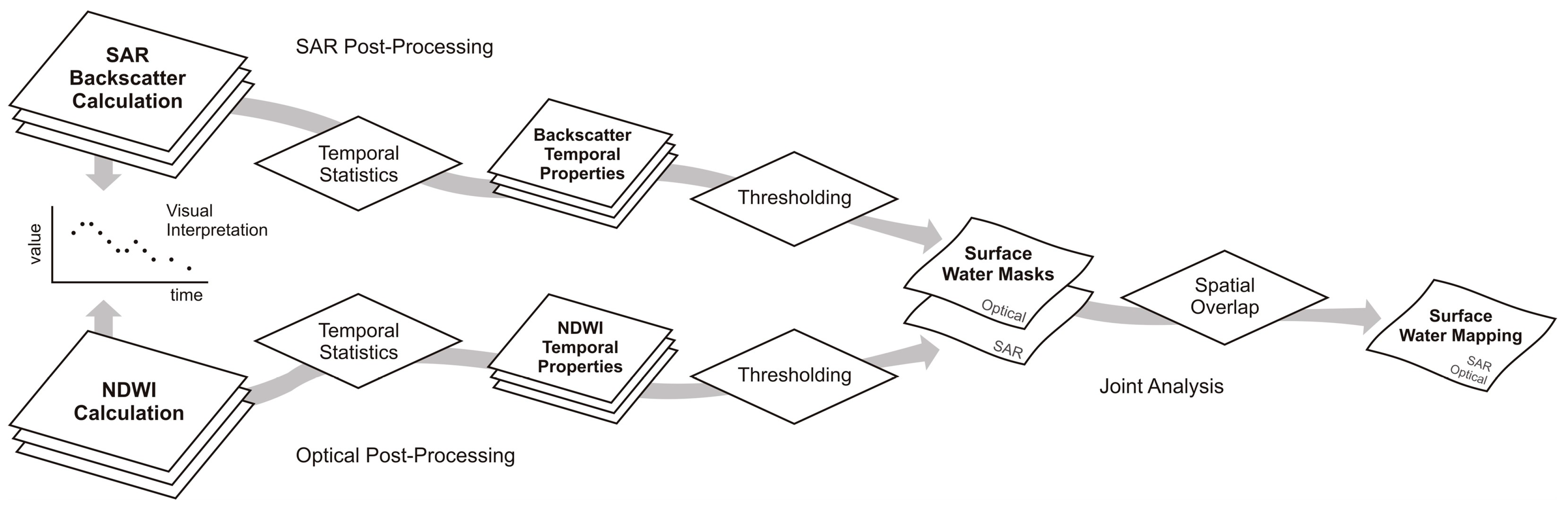
This study follows a time series analysis approach for surface water/flood mapping with the use of SAR backscatter intensity from the Sentinel-1 image archive acquired between September 2015 and May 2020 (244 S-1A and S-1B images, descending orbit 7). A well designed image processing chain (
Figure 2 and
Figure S3) was applied to the Sentinel-1 IW GRD datasets in order to extract geophysical information in proper map geometry. Specifically, the initial processing steps involved the update of orbit state vectors to improve geolocation accuracy and the radiometric calibration to sigma naught (sigma0). The calibrated sigma0 values (in dB) represent the normalized radar cross-section and describe radar reflectance properties per pixel. The data calibration compensates for the radiometric influences of the different incidence angles. Further steps included multilooking for speckle reduction and terrain correction (ortho-rectification) of the results. It is worth mentioning that only the co-polarized VV channel was considered in the analysis, as it was more appropriate for land applications. The Shuttle Radar Topography Mission (SRTM) 1 arc-second heights [
83] were used to transform SAR images from radar geometry into a selected map projection. The reduced spatial resolution (pixel size) of the outputs at 20 m was sufficient for the needs of the current work.
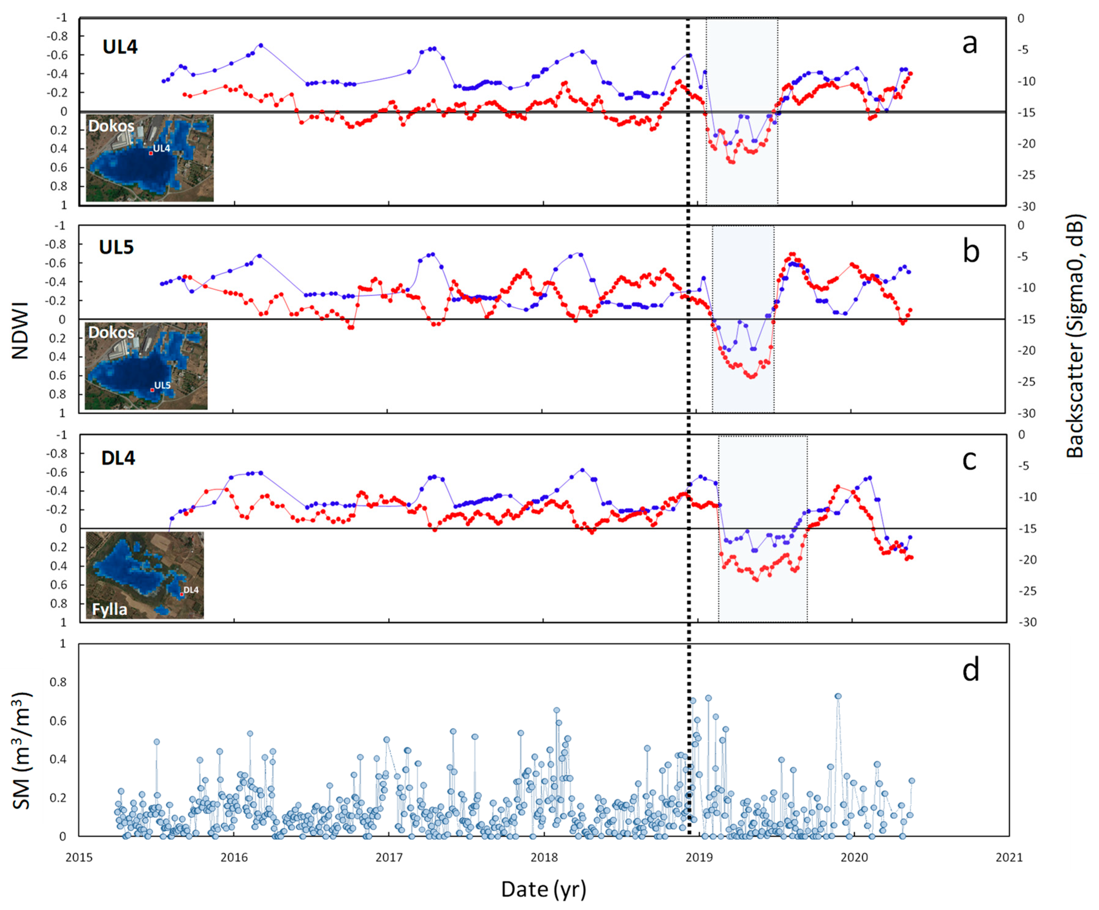
Using the Sentinel-1 backscatter time series (
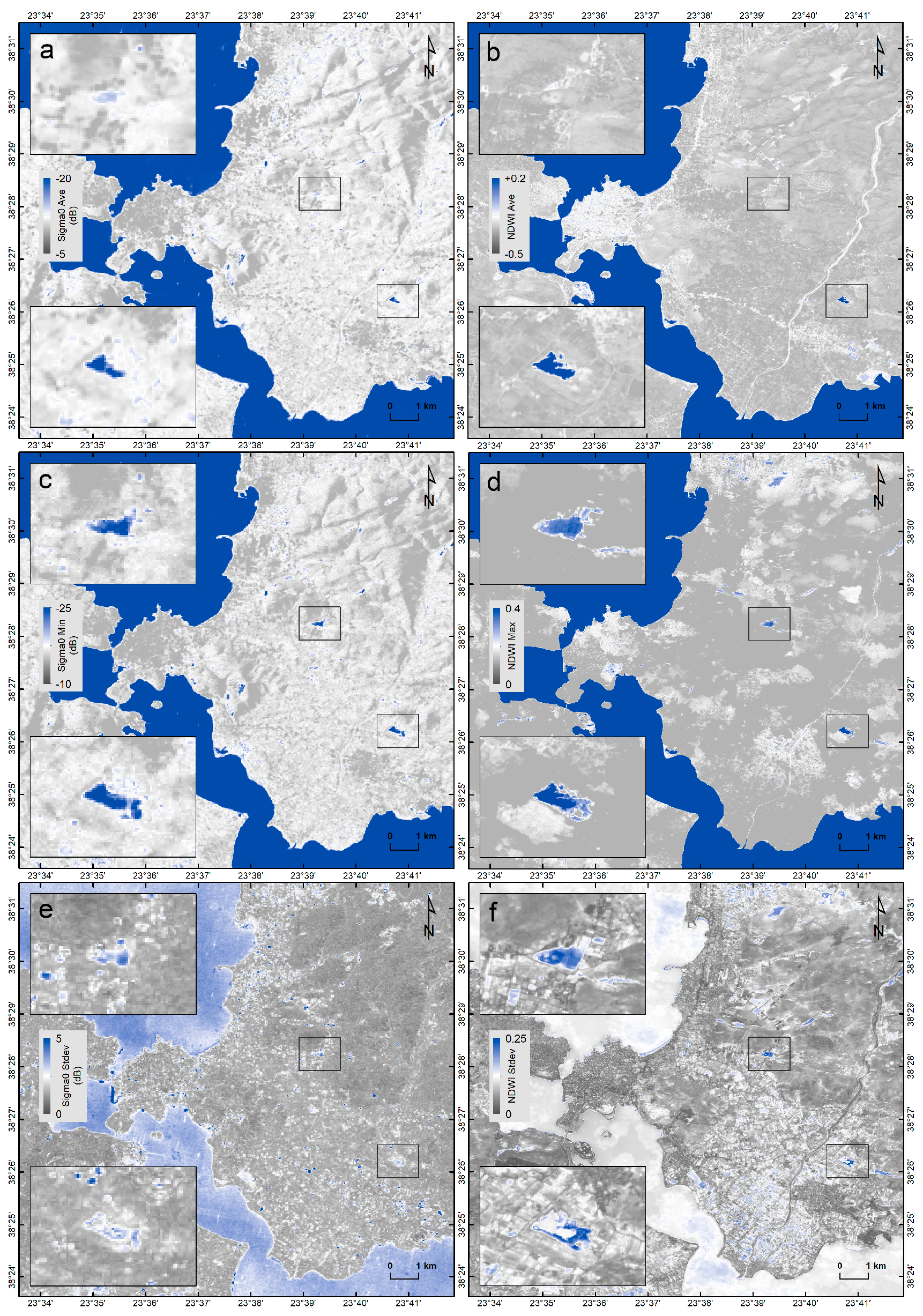
Figure 3), surface water changes were extracted in order to document the surface water dynamics in the area. Furthermore, the calculation of temporal statistics (minimum, maximum, average, and standard deviation), on a pixel basis and for the entire observation period, allowed for the study of the temporal variation in the backscatter, including seasonal or annual fluctuations related to normal water conditions (
Figure 4). The advantage of this methodology was the ability to detect persistent surface water, as well as to identify the exact period in and extent to which the flood occurred. It allowed for the identification of regions with a prolonged presence of surface waters (defined time span), separating them from permanent water bodies.
Therefore, according to the time series analysis, and by evaluating the backscatter variations between flood periods and normal water level conditions, it appears that similarity in the backscatter response provided a clear indication of the periods of flooding across the various sites (
Figure 5).
3.2. Sentinel-2 Time Series of Radiometric Indices
For the detection of increased water content and flood traces, the Copernicus Sentinel-2 mission has dedicated spectral bands in the visible green (B03) and near-infrared (B08) electromagnetic spectrum, with a 10 m spatial resolution, which make them suitable for delineating a flood’s extent.
Commonly applied methods used to extract water bodies from multispectral optical imagery are based on band indices specifically designed to enhance water content changes in a satellite image. A well performing method is the normalized difference water index (NDWI) developed by [
38], which relies on the combination of the near-infrared (NIR) and green spectral bands (see Equation (1)). This index has demonstrated its efficiency in water discrimination for various environments as water features have positive values and are enhanced, while vegetation and soil features usually have values of zero or negative ones, and are suppressed:
Sentinel-2 images were obtained for the period between July 2015 and May 2020 (119 S-2A and S-2B images, descending orbit 50), in Level-1C atmospheric top reflectivity products (top-of-atmosphere, TOA). The TOA L1C reflectance images were processed with the Sen2Cor [
84] processor algorithm using a combination of state-of-the-art techniques to perform atmospheric corrections, creating bottom-of-atmosphere (BOA) Level 2A (L2A) corrected reflectance images (
Figure 2 and
Figure S3). Since the spatial resolution of the near-infrared and green bands is equally 10 m, Sentinel-2 L2A images were directly stacked to finally obtain a water index image for each input image in a 10 m resolution and then create the long-term time series of the spectral properties (
Figure 6) for the purpose of studying the water trends, including seasonal or interannual patterns (
Figure 5).
From water pixel values (either spectral values or combinations of them, such as ratios or indices) of the time series statistical parameters were calculated, such as the minimum, maximum, mean, median, standard deviation, trend, etc. The temporal features of the average and maximum water coverage used in this approach are shown in
Figure 4. The temporal statistics are thus used to derive alternative features based on S-2 time series data that capture, in the best manner, the differences in the spectral behavior of the water extent over time.
3.3. SMOS- and EO-Based Precipitation
The ESA SMOS mission, launched in late 2009, determines, among other things, the surface soil moisture over land at a global scale. Knowledge of the spatiotemporal distribution of soil moisture is essential for various applications, such as water resource management, flood forecasting, and groundwater recharging. Soil moisture (SM) comprises an important hydrological and climatic parameter of the initial condition of the soil, and when combined with rainfall can provide valuable information for flood monitoring as well as prediction. SMOS provides soil moisture content to a depth of a few centimeters [
85], typically in the range of 0–5 cm, depending on the degree of soil wetness, and features a 2–3-day revisit time [
42].
For this study, SMOS Level 3 soil moisture data from March 2015 to May 2020 were selected with a 3-day temporal aggregation, which allows for the best estimation of SM when several multiorbit retrievals are available at a time [
86]. SMOS measurements were acquired along the ascending pass, since the retrievals of the top 5 cm from the early morning show better agreement with in situ measurements [
87,
88,
89,
90,
91]. In the ascending orbits (the early morning) the retrievals are more accurate, as the ionospheric effects are expected to be minimal and the surface conditions are close to thermal equilibrium [
86].
In addition to direct soil moisture estimates, satellite precipitation products were also utilized. In fact, although rain gauges provide the most accurate and direct measurement of precipitation, due to a lack of well-distributed in situ rain gauge measurements satellite precipitation products represent a reliable alternative for providing global information and operational facilities for rainfall estimates. Furthermore, recent studies assess how soil moisture measurements from space-based sensors can be used to improve satellite-based precipitation estimates [
92,
93,
94,
95,
96,
97,
98].
In this study, daily and monthly precipitation data were obtained from satellite measurements for the period between May 2015 and May 2020 through the Copernicus Climate Change Service (C3S) implemented by the ECMWF (European Centre for Medium-Range Weather Forecasts) and NASA Goddard Earth Sciences Data and Information Services Center (GES DISC). For rainfall-accumulated precipitation (in mm), the following products were used:
- (a)
GPM IMERG Final Daily Precipitation (GPM_3IMERGDF) [
99].
- (b)
GPM IMERG Final Monthly Precipitation (GPM_3IMERGM) [
100].
- (c)
TRMM TMPA/3B43 Monthly Rainfall Estimate [
101].
- (d)
Rainfall observations from the local network.
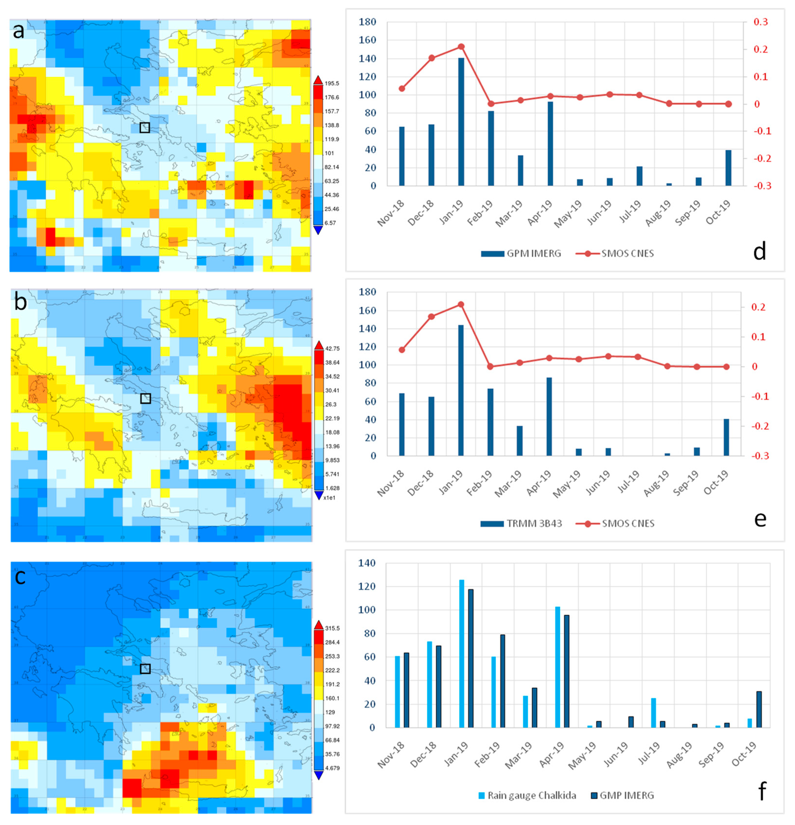
The precipitation data were jointly examined with SM measurements to derive the long-term changes in the meteorological conditions for the purpose of analyzing the 2019 flood event (
Figure 7). The time series of precipitation were compared with SMOS measurements for a chosen pixel containing the monitoring sites (
Figure 7). The time series indicate temporal consistency; in particular, an increase in soil moisture is observed following rainfall events, while maintaining lower values during spring and summer periods. This observation is important even though the amount of precipitation and the changes in soil moisture are not always proportional due to other controlling parameters, including surface runoff, drainage, intensive evaporation, the presence of vegetation, and different soil textures.
Furthermore, in situ observations from a single rain gauge station operating in the area, the Chalkida station (
Figure 1), located 4–8 km away from the study areas (
Figure 1), were obtained [
103] in order to assess the performance of satellite data. Between December 2018 and January 2019, the Chalkida station received, on average, 200–210 mm of rain (
Figure 7a,b), while the mean annual precipitation in the area does not exceed, on average, 290 mm. The high rainfalls can be clearly seen in the monthly precipitation time series for both the TRMM_3B43 and GPM IMERG estimates (
Figure 7d,e). Considering the in situ and satellite observations (
Figure 7f), they appear to be temporally strongly correlated, revealing that even though space-borne data have spatial resolutions of 10 km (GPM IMERG) and 25 km (TRMM_3B43), they happen to be consistent with site-specific rainfall heights.
Temporal satellite observations were able to provide supplementary, yet, as proven, independent sources of information concerning water inputs, contrary to in situ precipitation estimates, which are not always representative for the entire area considering the sparse monitoring stations (because of height differences, different geomorphological conditions, etc.).
4. Results
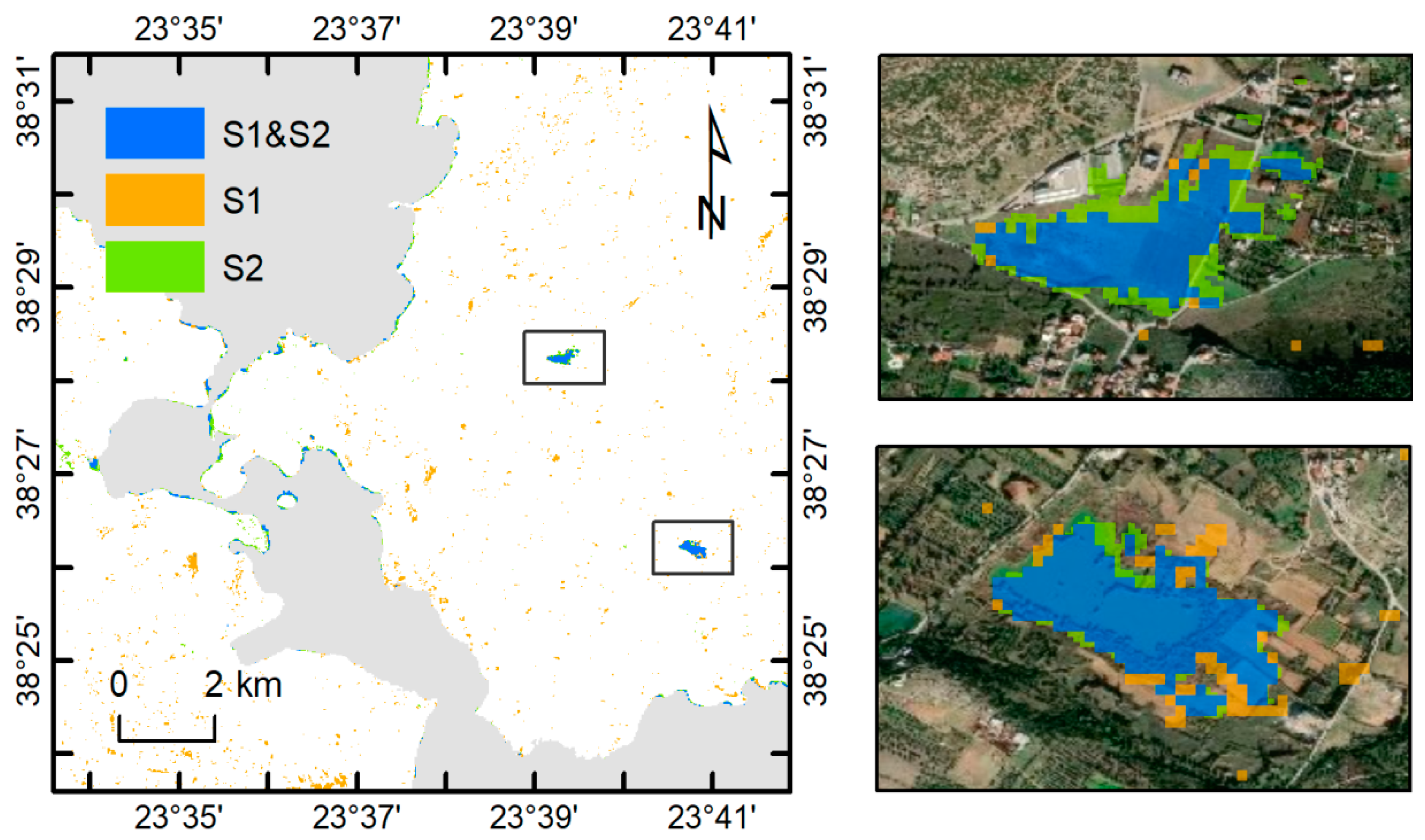
The multitemporal investigation on the period between 2015 and 2020 (
Figure 5) concerning two reference lakes, the ephemeral lake in Dokos and the permanent lake in Fylla, underlines the fact that they were inundated during the 2019 flood period. Both sites are located in the surficial sediments of the Lilas River alluvial plain and are in close proximity to WNW-SE-oriented outcrops of limestone (
Figure 1). Consistent temporal trends in the total estimated water area are observed between the different monitoring approaches (
Figure 5); however, the joint analysis allowed the exclusion of local outliers (mainly NDWI false positives), improving in this way the outputs and facilitating their proper interpretation. While the time series of the NDWI and SAR backscatter are consistent during inundation events, they may deviate for the remaining observation period (i.e., during ‘normal’ conditions), showing a low degree of correlation. In fact, both the NDWI and SAR backscatter can be used to detect water bodies, yet SAR observations are sensitive to variability in vegetation growth, among other factors, which introduces differences into their temporal patterns compared to the NDWI; however, by combining the NDWI and SAR, we obtain a more accurate estimate of the water presence and dynamics.
The evolution of the radar backscatter over the entire monitoring period of 2015–2020 shows significant temporal variability across the lake, yet consistent low backscatter values ranging between −15 dB and −25 dB suggest that the area was governed by water supply during the 2019 flood event. This backscatter minimum, which is evident in all of the time series, is comparable for the reference period, with the positive ratios of the NDWI time series indicating that the reference lakes were only temporally inundated; the constant presence of water is equal to 1 and the constant absence of water is equal to 0. This observation is consistent with the occurrence of an extreme rainfall event almost three months before the observed flooding, as recorded by satellite rainfall observations (
Figure 7) and soil moisture estimates (
Figure 5d). The high level of moisture during the period of intense rainfall indicates an increase in the water content on the land surface and further supports the occurrence of the flood event in early 2019.
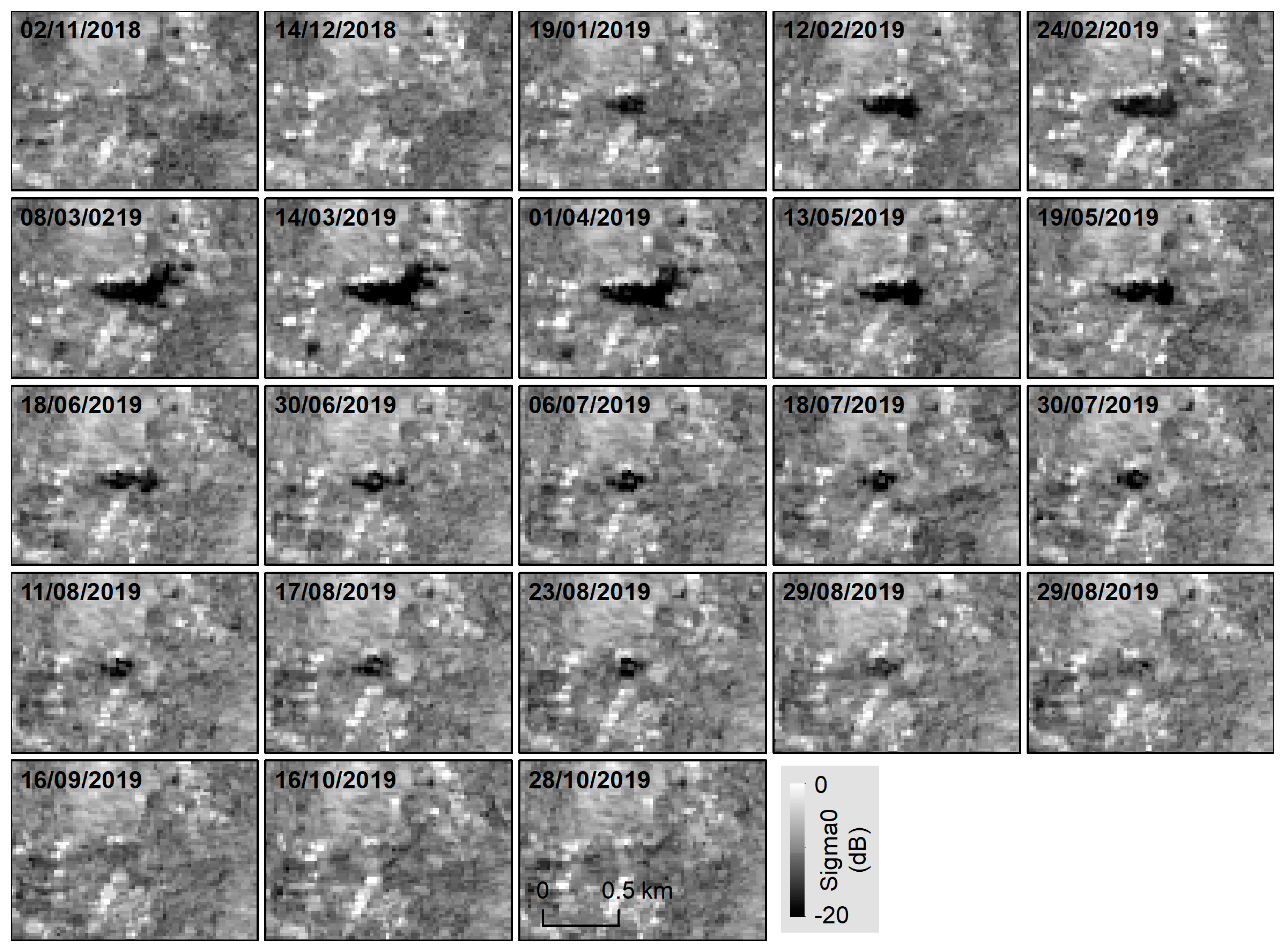
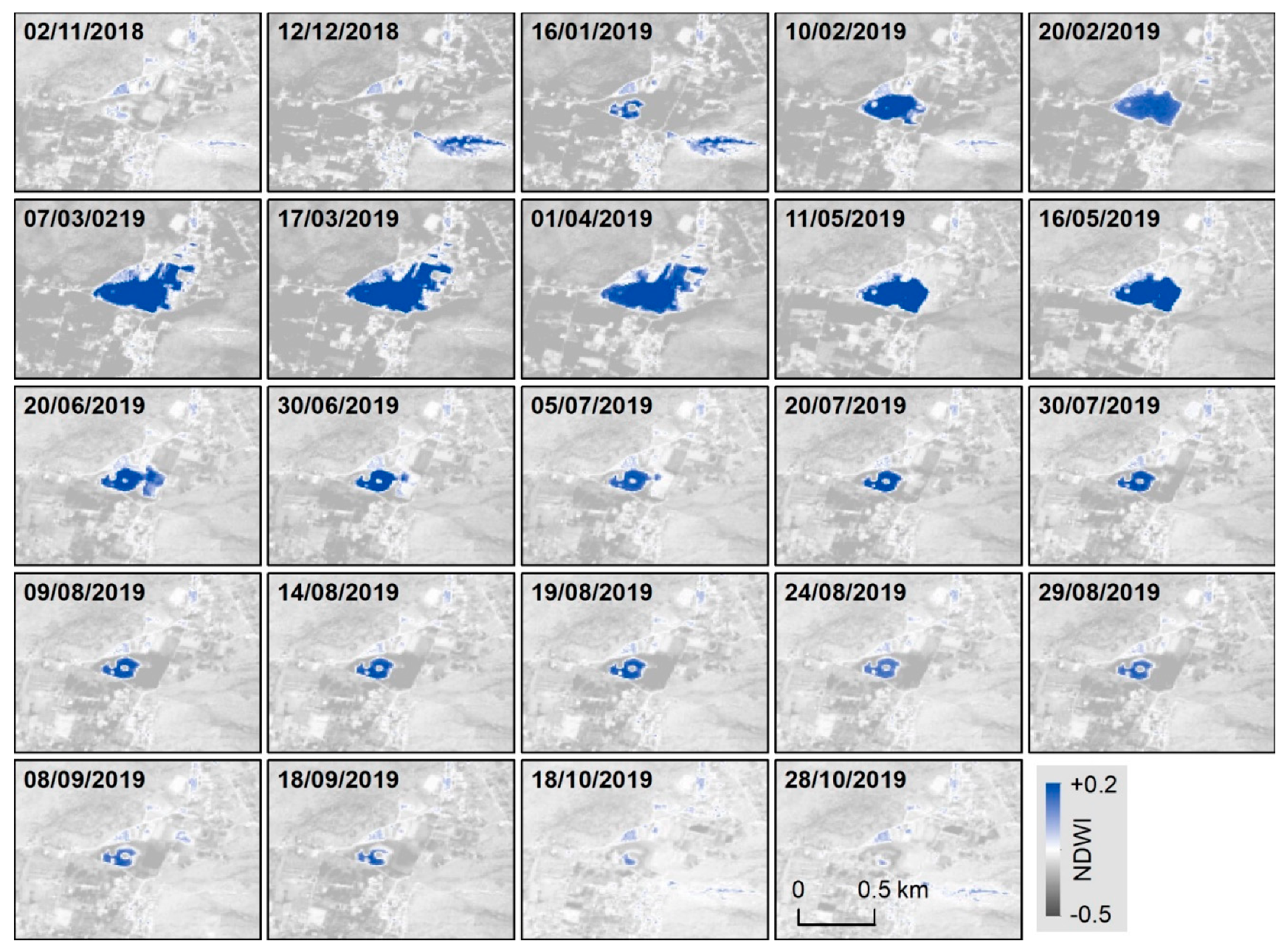
The spatiotemporal analysis of temporary surface water is chosen to be further presented for the Dokos lake in
Figure 3 and
Figure 6, as this lake was entirely formed during this flood episode. Surface water is first observed at the area on 16 January 2019, covering only a small part of the lake, the extent of which gradually increased in the following months, reaching its maximum coverage in March 2019. The visual interpretation with reference photos is shown in
Figure S1 [
104,
105]. From May 2019 the amount of water reduced significantly, and only the part of the former lake seemed to still possess water. The ephemeral lake progressively declined and disappeared completely in October 2019. The evolution of the spatial variability in the S-1 backscattering coefficient and the S-2 NDWI shows identical performance (
Figure 8).
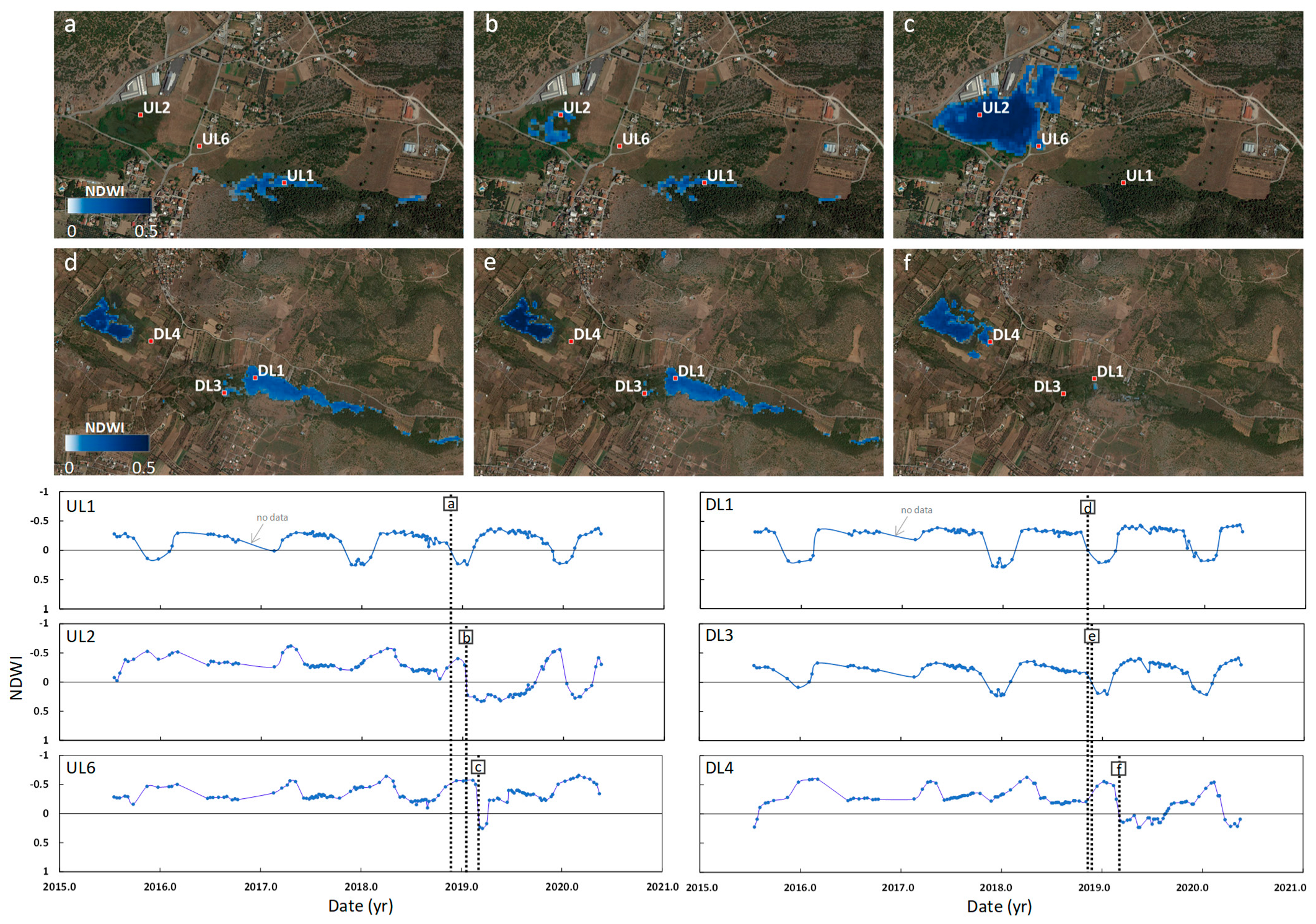
A noteworthy feature characterizes the former detection of water to the east of the Dokos lake on 12 December 2018 (site UL1,
Figure 9), around a month before the appearance of the ephemeral lake (on 16 Jan 2019), following the WNW-SE outcrops of kastic limestone, which could potentially be the means that controlled and supplied the karstic flood. This phenomenon appears to be identical for the Fylla lake, suggesting for both lakes the origin of karstic groundwater and the flow processes that caused flooding (
Figure 9). As described in
Figure 9, there seems to be a gradual water flow from the east (sites UL1 and DL1) that progressively supplies the lakes in a time window of approx. 3 months. This fact seems to follow a dependency relation in which the recharging of the lakes continues to increase, with the maximum extent of water in March 2019, until the water in the karstic outcrop finally disappears. Other flooding events, limited in the karstic limestone, have been also recognized in the NDWI time series, indicating seasonal effects during November and December; however, they did not result in analogous lake flooding in the area.
Although seasonal patterns are more evident in the NDWI time series, as the SAR backscatter is also affected by factors other than moisture content (mainly vegetation changes), with annual minima in late spring and early summer, an important fact remains that the reference area records the first considerable and long-lasting increase in surface water in early 2019, during the 5-year time span. The detailed investigation of SAR backscatter time series was therefore followed by examining their statistical properties to determine the impact of the flood event. The results are shown in
Figure 4. The standard deviation was computed based on the time series for each pixel, with the purpose of showing water variability. In this case, computing the standard deviation allows for the identification of areas that show strong variability exceeding expected seasonal behavior. Areas of such high deviations are indicative of water inundation, meaning that they were flooded during the 2019 event (
Figure 4).
According to the average, minimum (negative values for sigma naught in dB), and maximum (positive NDWI values) results (
Figure 4), the maximum water area change was observed in the northern ephemeral lake, whilst still considerable changes in the margins of the permanent southern lake were also noticed close to the flood peak date. Due to the lowland karst terrain, the maximum inundation areas were assumed to be associated with the storage capacity, as it is likely to hold the maximum water storage, hence lake basins. Note that the maximum water coverage of the two water bodies demonstrated similar local hydrological conditions that regulated inundation. The results highlight the suitability of the methods used for each satellite sensor.
5. Discussion
Data collected for approximately 5 years from different sensors with different spatial resolutions were processed, showing that, independently of the sensors’ characteristics and the applied processing chains, it is promising to obtain time series in qualitatively good agreement for contributing variables such as surface water. On the basis of satellite data (S-1 and S-2) mapping, surface water was effectively detected at a spatial resolution of 10–20 m, along with its long-term variation. Through this, it was also possible to identify water peaks related to the 2019 flood that are primarily associated with the ephemeral appearance of the Dokos lake to the north and the spreading of the permanent Fylla lake to the south (
Figure 9).
The multisource and multitemporal data analysis determined the extent as well as intensity of the flooding and revealed that the reference lakes recommend flood-prone areas that are most affected when weather-related extreme events occur without an annual repeatability.
Diverse remotely sensed data were integrated into a GIS environment for further analysis, specifically the definition and extraction of the flood-affected areas and co-interpretation along with the morphological as well as geological features of the area (
Figure 1). Both sites show great similarity since they lie in the alluvial fan deposits of the Lilas River, which allow rainfall to enter the karst system almost immediately. Furthermore, they are located next to limestone of the same WNW-SE orientation, suggesting the possibility of hydraulic connections between them. Any presence of favorable structural controls, such as dipping beds or folds, may also contribute to the accentuation of water flow. The limestone formations are located on the margins of the lowland karstic system and constitute the southern extension of the mountain masses found to the north. Coupled with the high rainfall levels for January 2019, both lakes’ vicinities with the relatively steep limestone hills seem to facilitate water flow between them; however, it is of great importance to understand the nature of the connection and the hydrological processes that prevailed between the floodplains and the water drainage system. It was shown that, during the rainfall peak in January 2019, localized water outflow partially covered the Dokos lake, while the time taken to reach the maximum outflow was in March 2019 (
Figure 3 and
Figure 6). This signifies that it took significantly longer to reach the maximum outflow, resulting in a prolonged flood duration. Indeed, despite the absence of rainfall during the spring and summer periods water levels have declined significantly, but flood waters are present. The maximum observed outflow may represent the maximum drainage capacity of the lakes under heavy rainfall conditions and should be considered for evaluating future extreme scenarios. The comparison of inundation with rainfall records for the same period shows a strong relationship between rainfall and flood dynamics, resulting in floodplains characterized by low-frequency and long-duration flooding. The spatially variable hydrodynamic properties and responses within the area helped in understanding that the underground karst flow is controlled by two discharge scenarios, the storage capacity of the lakes, and the floodwater that enters from proximal sources.
By means of satellite remote sensing, we were able to propose a flooding mechanism for both lakes, with the source of karst groundwater recharging initially at the east calcareous hills and progressively supplying the lakes with water via karst conduits and not surface runoff. Characteristically, in the case of the Dokos lake, the water seems to first discharge on the deeper western side of the lake, while it gradually increases to fill the shallower areas (
Figure 9). It is very interesting that water gradually fills the lakes, starting from its deeper part, almost three months following the heavy rainfalls. This delay, combined with the local absence of runoff during the flooding, implies that the phenomenon is controlled by a groundwater transfer mechanism. In parallel, runoff on the limestone, which appears immediately after the rainfall event, disappears in a relatively short time without any traces. In particular, surface runoff following the extreme rainfall is limited to the karstic limestone and disappears relatively fast. Then, after several months, surface water starts appearing at the deepest part of the nearby ephemeral lake, which, in time, leads to overflooding. This flooding is maintained for approximately nine months, implying its connection to non-surficial hydrologic processes. In karstic terrains, the subsurface flow and storage of water can lead to delayed or prolonged responses to rainfall events.
The above observations may support our suggestion of groundwater rise and basin inundation due to the transfer of groundwater from the karstic to free aquifer systems. The homogeneity of the flood mechanism identified in this lowland karst area reinforced the understanding of the local hydrological and hydrogeological processes operating during flood conditions. An important base of knowledge has arisen from the recent extreme flooding event due to the increasing availability of diverse remote sensing data that offered the potential to describe flood conditions accurately, while overcoming the lack of a local monitoring network. The methodologies adopted provide the ability to monitor the long-term spatial and temporal changes in surface water, and consequently flood events that could be effectively addressed for flood risk analysis purposes.
In conclusion, the Lilas plain is susceptible to flooding when water levels within the nearby karstic aquifer rise during periods of intense or prolonged rainfall, even at neighboring basins, forming ephemeral lakes that may last for several months; however, it should be noted that, after the appearance of the ephemeral lake, inundated areas expand over urban settlements, mainly along the coastal zone, leading, in turn, to damages and sometimes the need for evacuation (
Figure S1). In this case, the first indication of water lake outflow that insists on time (
Figure 9b) could potentially signify a subsequent severe flooding reaching nearby villages and should be considered as a precursor in order to take measures and prevent property as well as human losses. Therefore, this multi-EO data analysis provides a basic conceptualization of the factors controlling precipitation, inflow, and discharge in the Lilas plain, and a valuable insight tool that should be used for determining hazards associated with groundwater-induced flooding in Chalkida. This inherent disaster should be explicitly acknowledged within the public authorities to permit proper flood hazard assessments for future extreme events.
6. Conclusions
Hydrological processes are dynamic phenomena acting at different timescales; therefore, a proper monitoring scheme is required for the effective identification of changes in surface water conditions. Following the 2019 flood event at the broader area of Chalkida, the spatial distribution of and temporal variability in surface water were analyzed and interpreted over the years of 2015–2020. It was demonstrated that EO data can play a significant role in improving our capacity for mapping temporary water bodies and provide key hydrological mechanisms.
The accuracy of ephemeral surface water delineation, including flood-affected areas, was significantly improved through the joint assimilation of multitemporal satellite data (i.e., S-1 SAR and S-2 optical), rather than using individual satellite observations. By additionally integrating near-surface soil moisture from SMOS- and EO-based rainfall observations, more accurate estimates were achieved concerning the variability in surface water and the prevailing flooding mechanism that appears to be strongly controlled by the karst system.
Based on the joint analysis of diverse EO time series, the area has experienced a single noteworthy flood episode during the five-year monitoring period. The findings verify the primary appearance of water runoff along the karstic landscape with the onset of intense rainfall. As expected by the local geology, surface water runoff is quickly channeled through the underground karst system to the neighboring free aquifers on which ephemeral lakes develop. Whether heavy rainfall will lead to a flood event is highly associated with the prolonged and extended appearance of surface water in those ephemeral lakes.
Remote sensing from multiple satellite sensors offers a unique synoptic tool that is often unattainable by traditional local gauging networks. Our EO-supported findings may serve as indicators for flood alerts in future extreme precipitation events, supporting decision making and minimizing response times in cases of emergencies.
Supplementary Materials
The following supporting information can be downloaded at:
https://www.mdpi.com/article/10.3390/geohazards4020012/s1, Figure S1: Photographs showing the 2019 flooding event that hit Dokos [
104,
105]; Figure S2: Past water fluctuations in Dokos from Google Earth; Figure S3: Schematic diagram showing SAR and optical processing adopted for Sentinel-1 GRD and Sentinel-2 L1C data.
Author Contributions
Conceptualization, E.P. and M.F.; methodology, E.P. and M.F.; software, M.F.; validation, E.P.; formal analysis, M.F.; investigation, E.P.; writing—original draft preparation, E.P.; writing—review and editing, E.P., M.F. and A.M.; visualization, E.P. and M.F. All authors have read and agreed to the published version of the manuscript.
Funding
This research received no external funding.
Data Availability Statement
The data presented in this study are available on request from the corresponding author.
Acknowledgments
We would like to express our sincere appreciation to the anonymous reviewers for their insightful comments and suggestions, which greatly improved the quality of this manuscript. We also extend our gratitude to the Academic Editor for the careful editing and support throughout the review process.
Conflicts of Interest
The authors declare no conflict of interest.
References
- Coxon, C.E.; Drew, D.P. Interaction of surface water and groundwater in Irish karst areas: Implications for water resource management. In Gambling with Groundwater—Physical, Chemical and Biological Aspects of Aquifer–Stream Relations; Brahana, J.V., Eckstein, Y., Ongley, L.K., Schneider, R., Moore, J.E., Eds.; American Institute of Hydrology: St. Paul, MN, USA, 1998; pp. 161–168. [Google Scholar]
- Ford, D.; Williams, P. Karst Hydrogeology and Geomorphology; John Wiley: Chichester, UK, 2007; p. 562. [Google Scholar] [CrossRef]
- Drew, D.P. Hydrogeology of lowland karst in Ireland. Q. J. Eng. Geol. Hydrogeol. 2008, 41, 61–72. [Google Scholar] [CrossRef]
- Klove, B.; Ala-aho, P.; Bertrand, G.; Boukalova, Z.; Erturk, A.; Goldscheider, N.; Ilmonen, I.; Karakaya, N.; Kupfersberger, H.; Kvoerner, J.; et al. Groundwater dependent ecosystems. Part 1: Hydroecological status and trends. Environ. Sci. Policy 2011, 14, 770–781. [Google Scholar] [CrossRef]
- Bonacci, O. Poljes, ponors and their catchments. In Treatise on Geomorphology, Vol 6: Karst Geomorphology; Shroder, J., Frumkin, A., Eds.; Academic: San Diego, CA, USA, 2013; pp. 112–120. [Google Scholar] [CrossRef]
- Upton, K.A.; Jackson, C.R. Simulation of the spatio-temporal extent of groundwater flooding using statistical methods of hydrograph classification and lumped parameter models. Hydrol. Process. 2011, 25, 1949–1963. [Google Scholar] [CrossRef] [Green Version]
- Naughton, O.; Johnston, P.M.; Gill, L.W. Groundwater flooding in Irish karst: The hydrological characterization of ephemeral lakes (turloughs). J. Hydrol. 2012, 470–471, 82–97. [Google Scholar] [CrossRef]
- Bonacci, O.; Ljubenkov, I.; Roje-Bonacci, T. Karst flash floods: An example from the Dinaric karst (Croatia). Nat. Hazards Earth Syst. Sci. 2006, 6, 195–203. [Google Scholar] [CrossRef] [Green Version]
- Najib, K.; Jourde, H.; Pistre, S. A methodology for extreme groundwater surge predetermination in carbonate aquifers: Groundwater flood frequency analysis. J. Hydrol. 2008, 352, 1–15. [Google Scholar] [CrossRef]
- Diakakis, M.; Foumelis, M.; Gouliotis, G.; Lekkas, E. Preliminary flood hazard and risk assessment in Western Athens Metro-politan Area. In Advances in the Research of Aquatic Environment; Lambrakis, N., Stournaras, G., Katsanou, K., Eds.; Springer: Berlin/Heidelberg, Germany, 2011; Volume 1, pp. 147–154. [Google Scholar] [CrossRef]
- Tsitroulis, I.; Voudouris, K.; Vasileiou, A.; Mattas, C.; Sapountzis, Μ.; Maris, F. Flood hazard assessment and delimitation of the likely flood hazard zones of the upper part in Gallikos river basin. Bull. Geol. Soc. Greece 2016, 50, 995–1005. [Google Scholar] [CrossRef] [Green Version]
- Copernicus Water & Wetness (WAW). Available online: https://land.copernicus.eu/pan-european/high-resolution-layers/water-wetness (accessed on 20 February 2023).
- Copernicus Water Bodies Global. Available online: https://land.copernicus.eu/global/products/wb (accessed on 20 February 2023).
- Global Lakes and Wetlands Database (GLWD). Available online: https://www.worldwildlife.org/pages/global-lakes-and-wetlands-database (accessed on 20 February 2023).
- HydroSHEDS. Available online: https://www.hydrosheds.org/ (accessed on 20 February 2023).
- Global Reservoirs and Lakes Monitor (G-REALM). G-REALM—Home. Available online: https://www.usda.gov/ (accessed on 20 February 2023).
- Hoet, P.H.M.; Geys, J.; Nemmar, A.; Nemery, B. NATO Science for Peace and Security Series C, Environmental Security; Korgan, F., Powell, A., Fedorov, O., Eds.; Springer: New York, NY, USA, 2011. [Google Scholar]
- Klemas, V. Remote Sensing of Floods and Flood-Prone Areas: An Overview. J. Coast. Res. 2015, 31, 1005–1013. [Google Scholar] [CrossRef] [Green Version]
- Mouratidis, A.; Sarti, F. Flash-Flood Monitoring and Damage Assessment with SAR Data: Issues and Future Challenges for Earth Observation from Space Sustained by Case Studies from the Balkans and Eastern Europe. In Earth Observation of Global Changes; Springer: Berlin/Heidelberg, Germany, 2012; pp. 125–136. [Google Scholar] [CrossRef]
- Chini, M.; Giustarini, L.; Matgen, P.; Hostache, R.; Pappenberger, F.; Bally, F. Flood hazard mapping combining high resolution multi-temporal SAR data and coarse resolution global hydrodynamic modelling. In Proceedings of the 2014 IEEE Geoscience and Remote Sensing Symposium, Quebec City, QC, Canada, 13–18 July 2014; pp. 2394–2396. [Google Scholar]
- Parcharidis, I.; Lekkas, E.; Vassilakis, E. SIR-C/X Space Shuttle Images Contribution in Assessment of Flood Risk: The Case of Athens Basin. In Proceedings of the IEEE 2000 International Geoscience and Remote Sensing Symposium. Taking the Pulse of the Planet: The Role of Remote Sensing in Managing the Environment, Honolulu, HI, USA, 24–28 July 2000; pp. 328–330. [Google Scholar]
- Schlaffer, S.; Matgen, P.; Hollaus, M.; Wagner, W. Flood detection from multi-temporal SAR data using harmonic analysis and change detection. Int. J. Appl. Earth Obs. Geoinf. 2015, 38, 15–24. [Google Scholar] [CrossRef]
- Vickers, H.; Malnes, E.; Høgda, K.-A. Long-Term Water Surface Area Monitoring and Derived Water Level Using Synthetic Aperture Radar (SAR) at Altevatn, a Medium-Sized Arctic Lake. Remote Sens. 2019, 11, 2780. [Google Scholar] [CrossRef] [Green Version]
- Ruzza, G.; Guerriero, L.; Grelle, G.; Guadagno, F.M.; Revellino, P. Multi-Method Tracking of Monsoon Floods Using Sentinel-1 Imagery. Water 2019, 11, 2289. [Google Scholar] [CrossRef] [Green Version]
- Ogilvie, A.; Poussin, J.-C.; Bader, J.-C.; Bayo, F.; Bodian, A.; Dacosta, H.; Dia, D.; Diop, L.; Martin, D.; Sambou, S. Combining Multi-Sensor Satellite Imagery to Improve Long-Term Monitoring of Temporary Surface Water Bodies in the Senegal River Floodplain. Remote Sens. 2020, 12, 3157. [Google Scholar] [CrossRef]
- Doña, C.; Morant, D.; Picazo, A.; Rochera, C.; Sánchez, J.M.; Camacho, A. Estimation of Water Coverage in Permanent and Temporary Shallow Lakes and Wetlands by Combining Remote Sensing Techniques and Genetic Programming: Application to the Mediterranean Basin of the Iberian Peninsula. Remote Sens. 2021, 13, 652. [Google Scholar] [CrossRef]
- Hostache, R.; Matgen, P.; Wagner, W. Change detection approaches for flood extent mapping: How to select the most adequate reference image from online archives? Int. J. Appl. Earth Obs. Geoinf. 2012, 19, 205–213. [Google Scholar] [CrossRef]
- Clement, M.A.; Kilsby, C.G.; Moore, P. Multi-temporal synthetic aperture radar flood mapping using change detection. J. Flood Risk Manag. 2017, 11, 152–168. [Google Scholar] [CrossRef] [Green Version]
- Long, S.; Fatoyinbo, T.E.; Policelli, F. Flood Extent Mapping for Namibia using Change Detection and Thresholding with SAR. Environ. Res. Lett. 2014, 9, 3. [Google Scholar] [CrossRef]
- Pulvirenti, L.; Chini, M.; Pierdicca, N.; Boni, G. Use of SAR Data for Detecting Floodwater in Urban and Agricultural Areas: The Role of the Interferometric Coherence. IEEE Trans. Geosci. Remote Sens. 2016, 54, 1532–1544. [Google Scholar] [CrossRef]
- Matgen, P.; Hostache, R.; Schumann, G.; Pfister, L.; Hoffmann, L.; Savenije, H.H.G. Towards an automated SAR-based flood monitoring system: Lessons learned from two case studies. Phys. Chem. Earth 2011, 36, 241–252. [Google Scholar] [CrossRef]
- Pulvirenti, L.; Pierdicca, N.; Chini, M.; Guerriero, L. An algorithm for operational flood mapping from Synthetic Aperture Radar (SAR) data using fuzzy logic. Nat. Hazards Earth Syst. Sci. 2011, 11, 529–540. [Google Scholar] [CrossRef] [Green Version]
- Twele, A.; Cao, W.; Plank, S.; Martinis, S. Sentinel-1 based flood mapping: A fully automated processing chain. Int. J. Remote Sens. 2016, 37, 2990–3004. [Google Scholar] [CrossRef]
- Chini, M.; Giustarini, L.; Hostache, R.; Matgen, P. A hierarchical split-based approach for parametric thresholding of SAR images: Flood Inundation as a Test Case. IEEE Trans. Geosci. Remote Sens. 2017, 55, 6975–6988. [Google Scholar] [CrossRef]
- Pekel, J.; Cottam, A.; Gorelick, N.; Belward, A.S. High-Resolution Mapping of Global Surface Water and its Long-Term Changes. Nature 2016, 540, 418–422. [Google Scholar] [CrossRef]
- Aires, F.; Miolane, L.; Prigent, C.; Pham, B.; Fluet-Chouinard, E.; Lehner, B.; Papa, F. A Global Dynamic Long-Term Inundation Extent Dataset at High Spatial Resolution Derived through Downscaling of Satellite Observations. J. Hydrometeorol. 2017, 18, 1305–1325. [Google Scholar] [CrossRef]
- Acharya, T.D.; Subedi, A.; Lee, D.H. Evaluation of Water Indices for Surface Water Extraction in a Landsat 8 Scene of Nepal. Sensors 2018, 18, 2580. [Google Scholar] [CrossRef] [PubMed] [Green Version]
- McFeeters, S.K. The use of the Normalized Difference Water Index (NDWI) in the Delineation of Open Water Features. Int. J. Remote Sens. 1996, 17, 1425–1432. [Google Scholar] [CrossRef]
- Gao, B.C. NDWI—A Normalized Difference Water Index for Remote Sensing of Vegetation Liquid Water from Space. Remote Sens. Environ. 1996, 58, 257–266. [Google Scholar] [CrossRef]
- Xu, H. Modification of Normalised Difference Water Index (NDWI) to Enhance Open Water Features in Remotely Sensed Imagery. Int. J. Remote Sens. 2006, 27, 3025–3033. [Google Scholar] [CrossRef]
- Feyisa, G.L.; Meilby, H.; Fensholt, R.; Proud, S.R. Automated Water Extraction Index: A New Technique for Surface Water Mapping Using Landsat Imagery. Remote Sens. Environ. 2014, 140, 23–35. [Google Scholar] [CrossRef]
- Kerr, Y.H.; Waldteufel, P.; Wigneron, J.P.; Martinuzzi, J.M.; Font, J.; Berger, M. Soil moisture retrieval from space: The soil moisture and ocean salinity (SMOS) mission. IEEE Trans. Geosci. Remote Sens. 2001, 39, 1729–1735. [Google Scholar] [CrossRef]
- Lievens, H.; De Lannoy, G.J.M.; Al Bitar, A.; Drusch, M.; Dumedah, G.; Hendricks Franssen, H.-J.; Kerr, Y.H.; Tomer, S.K.; Martens, B.; Merlin, O.; et al. Assimilation of SMOS soil moisture and brightness temperature products into a land surface model. Remote Sens. Environ. 2016, 180, 292–304. [Google Scholar] [CrossRef] [Green Version]
- Seo, D.; Lakhankar, T.; Cosgrove, B.; Khanbilvardi, R.; Zhan, X. Applying SMOS soil moisture data into the National Weather Service (NWS)’s Research Distributed Hydrologic Model (HL-RDHM) for flash flood guidance application. Remote Sens. Appl. Soc. Environ. 2017, 8, 182–192. [Google Scholar] [CrossRef]
- Usowicz, B.; Lipiec, J.; Lukowski, M. Evaluation of Soil Moisture Variability in Poland from SMOS Satellite Observations. Remote Sens. 2019, 11, 1280. [Google Scholar] [CrossRef] [Green Version]
- Baugh, C.; de Rosnay, P.; Lawrence, H.; Jurlina, T.; Drusch, M.; Zsoter, E.; Prudhomme, C. The Impact of SMOS Soil Moisture Data Assimilation within the Operational Global Flood Awareness System (GloFAS). Remote Sens. 2020, 12, 1490. [Google Scholar] [CrossRef]
- Karymbalis, E.; Valkanou, K.; Tsodoulos, I.; Iliopoulos, G.; Tsanakas, K.; Batzakis, V.; Tsironis, G.; Gallousi, C.; Stamoulis, K.; Ioannides, K. Geomorphic Evolution of the Lilas River Fan Delta (Central Evia Island, Greece). Geosciences 2018, 8, 361. [Google Scholar] [CrossRef] [Green Version]
- CNN Greece. Available online: https://www.cnn.gr/ellada/story/168049/se-katastasi-ektaktis-anagkis-i-xalkida-egkataleipoyn-ta-plimmyrismena-spitia-toys-oi-katoikoi (accessed on 20 February 2023).
- Zorapas, M.; Sampatakaki, P.; Nikolaou, N. Preliminary Technical Report on Direct Demonstruction Projects of the Chalkida Area and the Municipality of Evia; Institute of Geology and Mineral Exploration (IGME), Address Hydrogeology: Athens, Greece, 2019. [Google Scholar]
- Golubovic-Deligianni, M.; Poulos, S.; Kotinas, V.; Panagou, T.; Alexopoulos, J. Investigation of the Causes of the Flooding in the Karst Areas of the Municipality of Halkida, Prefecture of Evia (Greece). In Proceedings of the 12th International Conference of Hellenic Geographical Society, Athens, Greece, 1–4 November 2019; Volume 1. [Google Scholar]
- Argyraki, A.; Pyrgaki, K. Technical Report on the Initial Conceptualisation and Characterisation of the Studied water Bodies in Greece; Faculty of Geology and Geoenvironment, National and Kapodistrian University of Greece: Zografou, Greece, 2018; 37p. [Google Scholar]
- Blackstock, T.H.; Duigan, C.A.; Stevens, D.P.; Yeo, M.J.M. Vegetation zonation and invertebrate fauna in Pant-y-Llyn, an unusual seasonal lake in South Wales, UK. Aquat. Conserv. Mar. Freshw. Ecosyst. 1993, 3, 253–268. [Google Scholar] [CrossRef]
- Ganoulis, J.; Vafiadis, M.M. Urban Flood Control in Karst Areas: The Case of Rethymnon (Greece). In Defence from Floods and Floodplain Management; NATO ASI Series; Gardiner, J., Starosolszky, Ö., Yevjevich, V., Eds.; Springer: Dordrecht, The Netherlands, 1995; Volume 299. [Google Scholar] [CrossRef]
- Hardwick, P.; Gunn, J. Landform–groundwater interactions in the Gwenlais karst, South Wales. In Geomorphology and Groundwater; Brown, A.G., Ed.; John Wiley: New York, NY, USA, 1995; pp. 75–91. [Google Scholar]
- López-Chicano, M.; Calvache, M.L.; Martín-Rosales, W.; Gisbert, J. Conditioning factors in flooding of karstic poljes: The case of the Zafarraya Polje (South Spain). Catena 2002, 49, 331–352. [Google Scholar] [CrossRef]
- Goodwillie, R.; Reynolds, J.D. Turloughs. In Wetlands of Ireland: Distribution, Ecology, Uses and Economic Value; Otte, M.L., Ed.; University College Dublin Press: Dublin, UK, 2003; pp. 130–134. [Google Scholar]
- Sheehy Skeffington, M.; Scott, N.E. Do turloughs occur in Slovenia? Acta Carsol. 2008, 37, 236–291. [Google Scholar] [CrossRef] [Green Version]
- Parise, M. Karst geo-hazards: Causal factors and management issues. Acta Carsolog. 2015, 44, 401–414. [Google Scholar] [CrossRef]
- Sarchani, S.; Tsanis, I. Analysis of a Flash Flood in a Small Basin in Crete. Water 2019, 11, 2253. [Google Scholar] [CrossRef] [Green Version]
- Ravbar, N.; Mayaud, C.; Blatnik, M.; Petrič, M. Determination of inundation areas within karst poljes and intermittent lakes for the purposes of ephemeral flood mapping. Hydrogeol. J. 2021, 29, 213–228. [Google Scholar] [CrossRef]
- Copernicus Open Access Hub. Open Access Hub. Available online: https://scihub.copernicus.eu/ (accessed on 20 February 2023).
- Centre Aval de Traitement des Données SMOS (CATDS). Available online: https://www.catds.fr/ (accessed on 20 February 2023).
- ESA SNAP Toolbox. STEP—Science Toolbox Exploitation Platform (esa.int). Available online: http://step.esa.int/main/ (accessed on 20 February 2023).
- Veci, L.; Lu, J.; Foumelis, M.; Engdahl, M. ESA’s Multi-mission Sentinel-1 Toolbox. In Proceedings of the 19th EGU General Assembly, EGU2017, Vienna, Austria, 23–28 April 2017; p. 19398. [Google Scholar]
- Horritt, M.S.; Bates, P.D. Predicting floodplain inundation: Raster-based modelling versus the finite-element approach. Hydrol. Process. 2001, 15, 825–842. [Google Scholar] [CrossRef]
- Henry Rotich, K.; Yongsheng, Z.; Jun, D. Municipal solid waste management challenges in developing countries—Kenyan case study. Waste Manag. 2006, 26, 92–100. [Google Scholar] [CrossRef] [PubMed]
- Matgen, P.; Schumann, G.; Henry, J.-B.; Hoffmann, L.; Pfister, L. Integration of SAR-derived river inundation areas, high-precision topographic data and a river flow model toward near real-time flood management. Int. J. Appl. Earth Obs. Geoinf. 2007, 9, 247–263. [Google Scholar] [CrossRef]
- Brisco, B.; Kapfer, M.; Hirose, T.; Tedford, B.; Liu, J. Evaluation of C-band Polarization Diversity and Polarimetry for Wetland Mapping. Can. J. Remote Sens. 2011, 37, 82–92. [Google Scholar] [CrossRef]
- Mason, D.C.; Davenport, I.J.; Neal, J.C.; Schumann, G.J.-P.; Bates, P.D. Near real-time flood detection in urban and rural areas using high-resolution Synthetic Aperture Radar images. IEEE Trans. Geosci. Remote Sens. 2012, 50, 3041–3052. [Google Scholar] [CrossRef] [Green Version]
- Martinis, S.; Kersten, J.; Twele, A. A fully automated TerraSAR-X based flood service. ISPRS J. Photogramm. Remote Sens. 2015, 104, 203–212. [Google Scholar] [CrossRef]
- Melack, J.M.; Wang, Y. Delineation of flooded area and flooded vegetation in Balbina Reservoir (Amazonas, Brazil) with synthetic aperture radar. J. SIL Proc. 1998, 26, 2374–2377. [Google Scholar] [CrossRef]
- Arnesen, A.S.; Silva, T.S.F.; Hess, L.L.; Novo, E.M.L.M.; Rudorff, C.M.; Chapman, B.D.; McDonald, K.C. Monitoring flood extent in the lower Amazon River floodplain using ALOS/PALSAR ScanSAR images. Remote Sens. Environ. 2013, 130, 51–61. [Google Scholar] [CrossRef]
- Chapman, B.; McDonald, K.; Shimada, M.; Rosenqvist, A.; Schroeder, R.; Hess, L. Mapping Regional Inundation with Spaceborne L-Band SAR. Remote Sens. 2015, 7, 5440–5470. [Google Scholar] [CrossRef] [Green Version]
- Zhao, L.; Yang, J.; Li, P.; Zhang, L. Seasonal inundation monitoring and vegetation pattern mapping of the Erguna floodplain by means of a RADARSAT-2 fully polarimetric time series. Remote Sens. Environ. 2014, 152, 426–440. [Google Scholar] [CrossRef]
- Pierdicca, N.; Chini, M.; Pulvirenti, L.; Macina, F. Integrating Physical and Topographic Information Into a Fuzzy Scheme to Map Flooded Area by SAR. Sensors 2008, 8, 4151–4164. [Google Scholar] [CrossRef] [PubMed] [Green Version]
- Frappart, F.; Seyler, F.; Martinez, J.-M.; León, J.G.; Cazenave, A. Floodplain water storage in the Negro River basin estimated from microwave remote sensing of inundation area and water levels. Remote Sens. Environ. 2005, 99, 387–399. [Google Scholar] [CrossRef] [Green Version]
- Pulvirenti, L.; Pierdicca, N.; Chini, M. Analysis of Cosmo-Sky Med observations of the 2008 flood in Myanmar. Ital. J. Remote Sens. 2010, 42, 79–90. [Google Scholar] [CrossRef]
- Badji, M.; Dautrebande, S. Characterisation of flood inundated areas and delineation of poor drainage soil using ERS-1 SAR imagery. Hydrol. Process. 1997, 11, 1441–1450. [Google Scholar] [CrossRef]
- Cian, F.; Marconcini, M.; Ceccato, P.; Giupponi, C. Flood depth estimation by means of high-resolution SAR images and lidar data. Nat. Hazards Earth Syst. Sci. 2018, 18, 3063–3084. [Google Scholar] [CrossRef] [Green Version]
- Schlaffer, S.; Chini, M.; Giustarini, L.; Matgen, P. Probabilistic mapping of flood-induced backscatter changes in SAR time series. Int. J. Appl. Earth Obs. Geoinf. 2017, 56, 77–87. [Google Scholar] [CrossRef]
- Betbeder, J.; Rapinel, S.; Corpetti, T.; Pottier, E.; Corgne, S.; Hubert-Moy, L. Multitemporal Classification of TerraSAR-X Data for Wetland Vegetation Mapping. J. Appl. Remote Sens. 2014, 8, 83648. [Google Scholar] [CrossRef]
- Tsyganskaya, V.; Martinis, S.; Marzahn, P.; Ludwig, R. Detection of Temporary Flooded Vegetation Using Sentinel-1 Time Series Data. Remote Sens. 2018, 10, 1286. [Google Scholar] [CrossRef] [Green Version]
- Farr, T.G.; Rosen, P.A.; Caro, E.; Crippen, R.; Duren, R.; Hensley, S.; Kobrick, M.; Paller, M.; Rodriguez, E.; Roth, L.; et al. The Shuttle Radar Topography Mission. Rev. Geophys. 2007, 45, RG2004. [Google Scholar] [CrossRef] [Green Version]
- Main-Knorn, M.; Pflug, B.; Louis, J.; Debaecker, V.; Müller-Wilm, U.; Gascon, F. Sen2Cor for Sentinel-2. In Proceedings of the Proc. SPIE 10427, Image and Signal Processing for Remote Sensing XXIII, Warsaw, Poland, 11–13 September 2017; p. 1042704. [Google Scholar]
- Bircher, S.; Skou, N.; Jensen, K.H.; Walker, J.P.; Rasmussen, L. A soil moisture and temperature network for SMOS validation in Western Denmark. Hydrol. Earth Syst. Sci. 2012, 16, 1445–1463. [Google Scholar] [CrossRef] [Green Version]
- Kerr, Y. CATDS SMOS L3 soil moisture retrieval processor algorithm theoretical baseline document (ATBD). CBSA, SO-TNCBSA-GS-0029. 2013. Available online: https://www.catds.fr/content/download/159115/file/SO-TN-CBSA-GS-0029_v3.pdf (accessed on 6 June 2022).
- Leroux, D.J.; Kerr, Y.H.; Al Bitar, A.; Bindlish, R.; Jackson, T.J.; Berthelot, B.; Portet, G. Comparison between SMOS, VUA, ASCAT, and ECMWF soil moisture products over four watersheds in US. IEEE Trans. Geosci. Remote Sens. 2014, 52, 1562–1571. [Google Scholar] [CrossRef] [Green Version]
- Jackson, T.J.; Bindlish, R.; Cosh, M.H.; Zhao, T.; Starks, P.J.; Bosch, D.D.; Seyfried, M.; Moran, M.S.; Goodrich, D.C.; Kerr, Y.H.; et al. Validation of Soil Moisture and Ocean Salinity (SMOS) Soil Moisture Over Watershed Networks in the U.S. IEEE Trans. Geosci. Remote Sens. 2012, 50, 1530–1543. [Google Scholar] [CrossRef] [Green Version]
- Dente, L.; Su, Z.; Wen, J. Validation of SMOS soil moisture products over the Maqu and Twente regions. Sensors 2012, 12, 9965–9986. [Google Scholar] [CrossRef] [PubMed]
- De Jeu, R. Retrieval of Land Surface Parameters Using Passive Microwave Remote Sensing. Ph.D. Dissertation, VU University, Amsterdam, The Netherlands, 2003; 122p. [Google Scholar]
- Draper, C.S.; Mahfouf, J.F.; Walker, J.P. An EKF assimilation of AMSR-E soil moisture into the ISBA land surface scheme. J. Geophys. Res. 2009, 114, D20. [Google Scholar] [CrossRef] [Green Version]
- Pellarin, T.; Ali, A.; Chopin, F.; Jobard, I.; Berges, J.C. Using spaceborne surface soil moisture to constrain satellite precipitation estimates over West Africa. Geophys. Res. Lett. 2008, 35, L02813. [Google Scholar] [CrossRef] [Green Version]
- Pellarin, T.; Román-Cascón, C.; Baron, C.; Bindlish, R.; Brocca, L.; Camberlin, P.; Fernández-Prieto, D.; Kerr, Y.H.; Massari, C.; Panthou, G.; et al. The Precipitation Inferred from Soil Moisture (PrISM) near Real-Time Rainfall Product: Evaluation and Comparison. Remote Sens. 2020, 12, 481. [Google Scholar] [CrossRef] [Green Version]
- Crow, W.T. A novel method for quantifying value in spaceborne soil moisture retrievals. J. Hydrometeorol. 2007, 8, 56–67. [Google Scholar] [CrossRef] [Green Version]
- Wanders, N.; Pan, M.; Wood, E.F. Correction of real-time satellite precipitation with multi-sensor satellite observations of land surface variables. Remote Sens. Environ. 2015, 160, 206–221. [Google Scholar] [CrossRef]
- Louvet, S.; Pellarin, T.; Al Bitar, A.; Cappelaere, B.; Galle, S.; Grippa, M.; Gruhier, C.; Kerr, Y.; Lebel, T.; Mialon, A.; et al. SMOS soil moisture product evaluation over West-Africa from local to regional scale. Remote Sens. Environ. 2015, 156, 383–394. [Google Scholar] [CrossRef]
- Zhan, W.; Pan, M.; Wanders, N.; Wood, E.F. Correction of real-time satellite precipitation with satellite soil moisture observations. Hydrol. Earth Syst. Sci. 2015, 19, 4275–4291. [Google Scholar] [CrossRef] [Green Version]
- Zhang, Z.; Wang, D.G.; Wang, G.L.; Qiu, J.X.; Liao, W.L. Use of SMAP Soil Moisture and Fitting Methods in Improving GPM Estimation in Near Real Time. Remote Sens. 2019, 11, 368. [Google Scholar] [CrossRef] [Green Version]
- Huffman, G.J.; Stocker, E.F.; Bolvin, D.T.; Nelkin, E.J.; Tan, J. GPM IMERG Final Precipitation L3 1 Day 0.1 Degree x 0.1 Degree V06; Savtchenko, A., Ed.; Goddard Earth Sciences Data and Information Services Center (GES DISC): Greenbelt, MD, USA, 2019. [CrossRef]
- Huffman, G.J.; Stocker, E.F.; Bolvin, D.T.; Nelkin, E.J.; Tan, J. GPM IMERG Final Precipitation L3 1 Month 0.1 Degree x 0.1 Degree V06; Goddard Earth Sciences Data and Information Services Center (GES DISC): Greenbelt, MD, USA, 2019. [CrossRef]
- Tropical Rainfall Measuring Mission (TRMM). TRMM (TMPA/3B43) Rainfall Estimate L3 1 Month 0.25 Degree x 0.25 Degree V7; Goddard Earth Sciences Data and Information Services Center (GES DISC): Greenbelt, MD, USA, 2011. [CrossRef]
- Acker, J.G.; Leptoukh, G. Online Analysis Enhances Use of NASA Earth Science Data. Eos Trans. Am. Geophys. Union 2007, 88, 14–17. [Google Scholar] [CrossRef]
- Meteo. Meteo View. Available online: https://stratus.meteo.noa.gr/index.php/ (accessed on 20 February 2023).
- Flood in Chalkida (tanea.gr). Available online: https://www.tanea.gr/2019/03/06/greece/i-plimmyra-sti-xalkida-se-eikones/ (accessed on 20 February 2023).
- Chalkida Floods. Available online: https://www.eviazoom.gr/2019/03/plummires-xalkida-paramenei-aperanti-limni-o-dokos.html (accessed on 20 February 2023).
| Disclaimer/Publisher’s Note: The statements, opinions and data contained in all publications are solely those of the individual author(s) and contributor(s) and not of MDPI and/or the editor(s). MDPI and/or the editor(s) disclaim responsibility for any injury to people or property resulting from any ideas, methods, instructions or products referred to in the content. |
© 2023 by the authors. Licensee MDPI, Basel, Switzerland. This article is an open access article distributed under the terms and conditions of the Creative Commons Attribution (CC BY) license (https://creativecommons.org/licenses/by/4.0/).


