1. Introduction
The impact of a tsunami can be devastating, both on human lives and economically. Some recent works [
1] show us how the impact of tsunamis has increased in the last few years, with a total of 251,770 casualties and USD 280 billion in damages between 1998 and 2017. For this reason, among others, there exist tsunami early warning systems (TEWS), and it is of key importance to continuously improve them.
The two main variables these systems must try to accurately anticipate are the maximum height of the incident waves and the arrival time of those. In this work, we will discuss how by taking advantage of deep learning techniques we can provide extremely fast and accurate predictions of these two variables.
Nowadays, there exist very efficient computer codes, implemented in massive parallel architectures as GPUs (graphics processing units), that return very accurate results in quite short computing times. Nevertheless, the computational resources required to include the variability associated with the uncertainty in the seismic source are still quite large and national TEWS do not have these resources available. In addition, even for a single “most probable” or “worst-case” scenario, depending on the level of conservatism, we may want to drastically reduce the time-to-solution. Here is where machine learning, or more concretely, deep learning, come into action. However, neural networks (NN) require large amounts of data to be trained, and regarding tsunamis, which are rare events, few data are available from natural events. Therefore, we lack the first main ingredient for building the model. Nevertheless, we can use our traditional computer tsunami models to generate the huge amount of data required to train NN. In addition, we can combine several NN models to produce more accurate results. Once the NN model is trained, it can be used to predict the maximum height and the arrival time for a particular event in just a few seconds.
Machine learning (ML) techniques are quickly spreading and being used in all fields of research, and tsunami science is not an exception. Many authors are starting to use ML techniques for tsunamis ([
2,
3,
4,
5,
6]).
In this paper, multi-layer perceptron (MLP) neural networks [
7] will be used to forecast tsunami maximum height and arrival time at certain points on the Chipiona-Cádiz coast (southwestern Spain). First, we considered single models and they produced good results. Next, in order to improve the results of those single models, ensemble techniques were also considered and implemented to reduce the variance of the results obtaining, in general, better predictions.
The present work is organized as follows:
Section 2 describes the context in which the present work arises and the simulations that will serve to train the NN models;
Section 3 briefly describes the NN models to be used; the single NN models proposed are described in
Section 4 and the numerical results obtained using single and ensemble models are presented in
Section 5;
Section 6 briefly describes how the basic tool proposed in this work could be used as building blocks of a real operational TEWS; and finally
Section 7 is devoted to highlighting some concluding remarks.
2. Motivation and Training Data
The aim of this work is to generate alert levels for a tsunami event in a very short time (seconds). Nowadays, in TEWS in Europe, this is still performed using decision matrices, a rudimentary approach, not considering local effects, nonlinearities of the phenomena, or even large masses of land preventing the tsunami wave reaching certain regions. In order to include a numerical approach in these systems, databases of precomputed scenarios are generated. When an event occurs, the system searches for a best-fit scenario in the database to be used as a model for the actual event. The main disadvantage of such a system relies on unexpected events not included in the database. Finally, few systems include FTRT (faster than real time) tsunami simulations on-the-fly of one or several deterministic scenarios produced in few minutes. This is achieved at IGN in Spain or CAT-INGV in Italy using the Tsunami-HySEA code.
Here, we propose to use ML techniques and NN models to generate the alert levels in few seconds. This paper will work on two regression problems. They consist of one predicting the maximum water height, and the other one predicting the arrival time of a tsunami at certain points in the coast. Here, we consider the Chipiona-Cádiz coast (segment CA01 in
Figure 1).
The Tsunami-HySEA code, developed by the EDANYA group at the University of Málaga, Spain, was used for the tsunami simulations [
8,
9]. The Okada model [
10] is used to compute the initial seafloor deformation caused by the earthquake. Tsunami-HySEA is currently being used in the TEWS of several countries (Spain, Italy, Chile), and it has been widely tested and benchmarked [
9,
11,
12].
For this study, we selected the Horseshoe fault as the seismic source, that is, the fault where the earthquake generating the tsunami is produced. This means that we are designing an NN model for tsunamis generated by this particular fault. As the aim of the present study is to define a methodological approach that can be used in any marine region with the potential of generating tsunamis, the method proposed here would have to be replicated for each active fault in the area of study in order to cover all the potential seismic tsunamigenic sources. Therefore, the choice of the particular fault we use in the present study is, in some sense, not really important. In any case, we chose the Horseshoe fault because it is supposed to be the source for the major event in the region, the Lisbon 1755 earthquake and tsunami [
13].
In
Table 1, we have listed the Okada model parameters and specified the range of values considered for each of the parameters. To generate the actual values within this range used to produce the numerical simulations, a Sobol sequence [
14] with 16,000 samples was used. Then, the Tsunami-HySEA model is used to simulate the 16,000 scenarios.
In order to have a finer resolution at the coast, the simulations were performed using three levels of nested grids. Grid level 0 has a spatial resolution of 320 m and 2,981,518 volumes, grid level 1 is 160 m and has 701,668 volumes, and grid level 2 is 40 m and is composed of 1,277,952 volumes. The size of the problem to be solved is 4,961,138 volumes in three spatial resolutions, and every single simulation takes approximately 280 s in a single GPU NVIDIA V100. This means that 1245 GPU computing hours are required. If we have access to a modest 64 GPU cluster, this can be computed in less than 20 h. If we have dedicated access to the whole MARCONI100 at CINECA, the Italian Supercomputer Center, (with 800 nodes and 3200 V100 GPUs, this would take less than 25 min.
For the present work, we selected six points, located on the segment of the coast named CA01 in
Figure 1. The maximum wave height and the arrival time of the first wave are going to be predicted by the NN model in these six points. They are located close to Sanlúcar de Barrameda, Chipiona, Arriates, the Arroyo Hondo river mouth, Rota, and Cádiz (see
Figure 2). The geographical coordinates for these points and the model-interpolated depths are collected in
Table 2.
We made the assumption that the tsunami arrives to a certain cell when the water level differs by 0.5 cm at that cell with respect to the initial water level, that is, if 0.5 cm, where and are the current and the initial water level, respectively.
In order to visualize the numerical results that are obtained for any of the large number of numerical simulations that we performed, we considered a particular seismic event, defined by the parameters in
Table 3. This scenario plays no particular role in the construction of the NN models presented in this work. We consider it to show the outputs extracted from each simulation used to train the NN models. In addition, in
Figure 3, the time series for the water height at the six forecast locations for this event are presented. Values for the time series were extracted every 5 s during 4 h.
Different regression techniques were implemented and tested, such as decision trees or random forest. Nevertheless, the predictions were not good enough to retain these models. Therefore, deep learning was used to predict the maximum height and arrival times in the minimum time possible, obtaining, at the same time, a very good accuracy.
3. Neural Network and Ensemble Learning
Before presenting the forecast obtained with the NN, a brief explanation of how a neural network works, its structure, what the ensemble used for training is, why it works well in practice, and what type of ensemble has been used will be given. Nevertheless, a discussion about the different types of activation functions, back-propagation, error functions, optimizers, regularizations, callbacks, etc., will be not given. More information about these concepts can be found in [
15,
16,
17,
18].
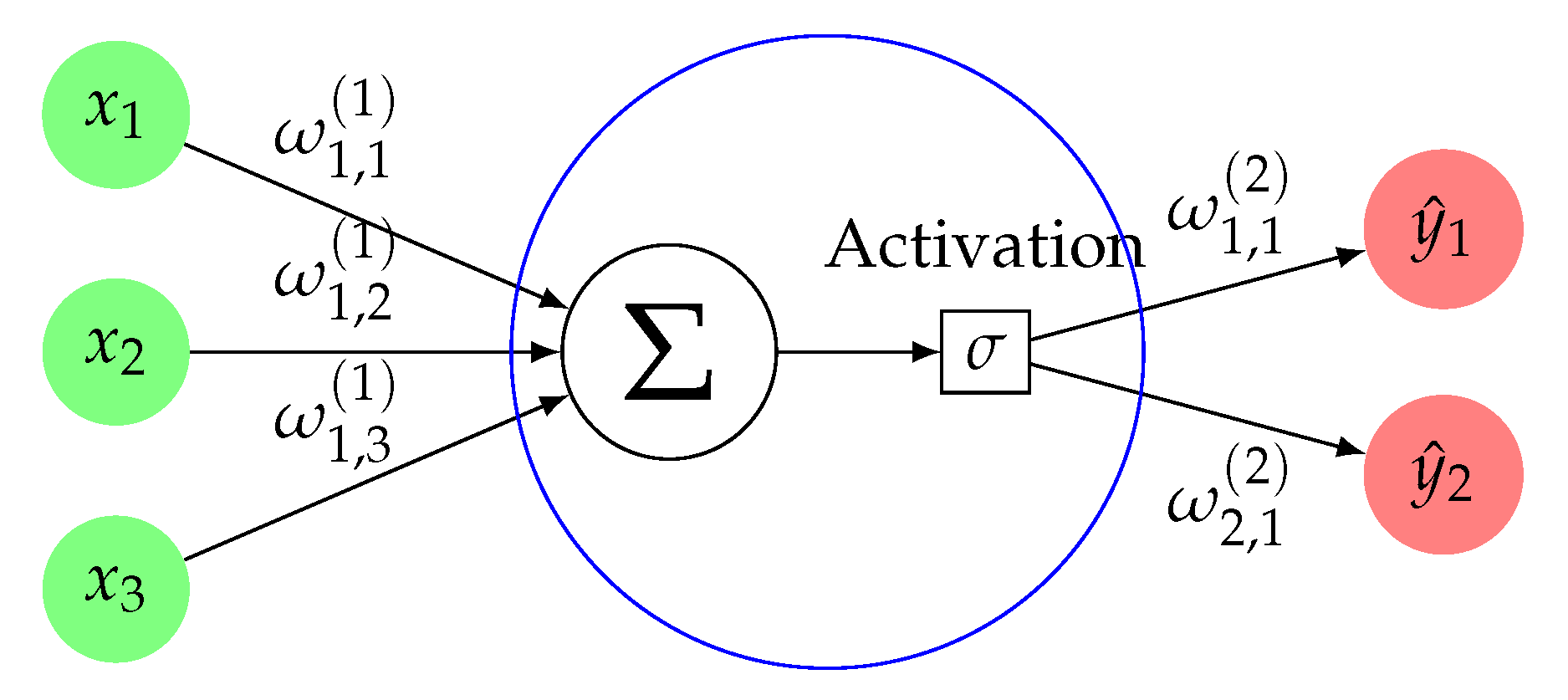
MLP neural networks were used to address the two problems considered in the present study. The type of neural networks that we used have a similar structure to the one shown in
Figure 4, but with more hidden layers and more neurons per hidden layer. We can think of the
as the Okada parameters (normalized to [0, 1]), and
as the results of each sample once forward-propagation is applied. The
values will be changing thanks to the use of back-propagation [
16]. When the last epoch is over, these
will be the result returned by the trained neural network. The term epoch refers to the number of passes the algorithm has completed through the entire training dataset.
As we can see, neural networks work similar to a human neuron; they receive the data, they process it, and, finally, a result is returned, but how does the neural network process the data? It takes two steps per layer. First, it combines, linearly, the output of the previous layer (input of the actual layer) and the synaptic weights,
. These weights are the values that the network will learn trying to find the best prediction. The resulting value will be denoted by
z, and it is called
net income. In the second step, an activation function [
17],
, is applied to the net income in order to determine the output of the layer. The activation functions are the ones which remove the linearity. Each layer has their own activation function. Visually, it can be seen in
Figure 5.
Therefore, defining as
the matrix of weights that connect to the layer
l, the net income,
, and the output,
, the output can be written matricially as
If we have several neural networks trained to solve the same problem, we could think to combine them to obtain better predictions. This is called ensemble learning. Ensemble learning follows the principle of “the wisdom of the crowd”, which shows that a large group of people with average knowledge on a topic can provide reliable answers to questions such as predicting quantities, spatial reasoning, and general knowledge. The aggregate results cancel out the noise and can often be better than those of highly trained systems. Ensemble learning combines several individual models to obtain better generalization performance. The reason why ensemble learning is efficient is because each model obtains different results. Each model might perform well on some data and less accurately on others. Variance is reduced to make better predictions.
There are many types of ensemble methods [
19,
20]. In our case, we used a weighted ensemble, which allows us to set for each model a weight (the contribution of the model in the ensemble). We need to define a list of new weights,
(they are different from the weights of the neural network we mentioned above). This list is filled with values we can give manually (grid search) or randomly (random search).
The elements of the list
are combined with all, considering all the possible
n-tuples, where
n is the number of models in our ensemble. Then, these
n-tuples are normalized to
. We have lots of possibilities, specifically,
, where
N is the dimension of vector
. We can choose an arbitrary
N, taking into account that a higher value will have a higher computational cost. As observation, it could happen that all weights are 0, then we have to discard this option. Thus, if we have
n models,
,
, and we denote by
E the ensemble learning, it writes as follows:
where
is the obtained result from model
, and
is the weight, once normalized, associated with the results of model
.
4. A First Approach: Single Neural Network Models
In this section, some neural network models that were trained, and that are similar to the selected final model used in this work, are described. Other techniques were tried too, producing worse results. We show some samples from networks with good results, where we can also observe the influence of certain parameters. The section is divided in two parts, one for the tsunami maximum height problem and another for the arrival times problem. We use the infinity norm to compute the difference between the predicted and true value. To contextualize these differences, maximum heights obtained by the simulations take values between 0.21 m and 3.47 m, and arrival times vary between 2565 s and 5504 s. For both problems, the 16,000 samples computed are randomly split in 12,000 samples for the training set, 2000 for the validation set, and 2000 for the test set. The training or train set is the portion of data used to fit the NN model. The validation set is used to improve the model; it is used to evaluate the model at the same time the model is being trained, but the validation data are not used to train the model. The validation set can be seen as a “weak training set”. Finally, the test set works as new data for the already trained model and is used to assess model accuracy. The best model is the one that minimizes the error in infinity norm, in our case for the maximum wave height or the arrival time, depending on the problem.
We used the Keras library [
21] to implement and train the NN models proposed in this work.
4.1. Models for Maximum Heights
A large set of single neural networks were trained in order to predict the maximum height of a tsunami at six points, and the resulting predictions were tested. These points are located around the coast between Chipiona and Cádiz, see
Section 2. Among the long list of models trained, in this section we include 24 models that are summarized in
Table 4,
Table 5 and
Table 6. The description and results of some selected trained models will be presented in the next section.
In
Figure 6, the maximum height in the high-resolution mesh of 40 m for the reference scenario in
Table 3 is depicted.
For each model presented, the inputs (the nine Okada parameters) were normalized to [0, 1]. The output layer has six neurons and the output was normalized to [0.02, 0.98]. In most of the models presented, the
Huber loss function [
21] with a threshold,
, equal to 0.1 is considered. The
Huber loss function is a piecewise function quadratic for small values of the residuals, and linear for large values, with equal values and slopes where the absolute value of the residuals equals the threshold. In other words, the
Huber loss function is defined as the mean squared error loss function (
mse) for values smaller than
and as the mean absolute error (
mae) loss function for values higher than
. The reason for this partition is to handle outliers. Mean squared error is smooth around 0, not increasing the error of predictions that are in this range, while mean absolute error has different gradients next to 0 and it may start oscillating with small errors. In addition,
mse is more influenced by extremes than
mae. The choice of the threshold
becomes important depending on what is considered an outlier.
To clarify this explanation, we provide the
Huber loss formula:
The learning rate is a configurable hyperparameter, used in the training of neural networks, that has a small positive value, in the range between 0.0 and 1.0, and it is one of the most crucial parameters [
22]. The step size or the
learning rate is the amount that the weights are updated during training. In the NN models described here, a learning rate of 0.002 returned better results than other learning rates. Models with a learning rate of 0.001 are also included. Regarding the batch size [
18] used in the models presented (the batch size is the number of samples processed before the model is updated), different batch sizes were tested, obtaining the best results with a value of 256 samples. Models with batch sizes of 128 and 512 are also presented.
The set of models that are presented were organized into three subsets, briefly described in
Table 4,
Table 5 and
Table 6. All the models presented use the
Adam algorithm as optimizer [
18] and the
early stopping callback [
21]. The models in
Table 4 have a sigmoid as activation function [
17] in the output layer. The
ReduceLROnPlateau callback [
21] was added in models in
Table 5. It improved the results. Finally, models without the sigmoid activation function in the output layer were developed. Results are presented in
Table 6.
Other popular activation functions, such as
relu [
17], different types of initialization weights, and different regularization techniques [
15], such as
Dropout,
L1,
L2, and
Batchnormalization, were also used, but in no case did the results improve.
Some of the models have a maximum height absolute error close to 7 cm and, in particular, model 23 has a maximum error of 6.7 cm or 6.8 cm for model 21. As model 23 presents the smaller value for the maximum, we will retain this model when using a single model NN. Other models, which also return good results (marked in blue), will be used in ensembles. The single models selected for the ensemble modeling do not have to be all of the models presenting the smaller maximum errors; it is important to select different models performing well in different situations. This justifies the choice of model 19.
4.2. Models for Arrival Times
In the same way as the NN, for predicting the maximum height at the forecast points, a second set of models was trained for the arrival times at the same six forecast points. In
Figure 7, the graphic for the simulated arrival times for the reference simulation is shown.
Inputs were normalized to [0, 1]. The output layer has six neurons, and in this case, the output was normalized to [0.05, 0.95]. The models in
Table 7 have no activation function in the output layer and use the
Adam algorithm as optimizer.
Early stopping and
ReduceLROnPlateau callbacks are used, too. Models without
ReduceLROnPlateau callback were developed and provided worse results.
Table 8 presents these results.
Our criterion will be to choose the green model from
Table 7 despite that we observed that it has a slight overfitting. This means that the model is very good at predicting the data used to train the model, but is not so good at predicting the data it was not trained on. Therefore, to avoid this, regularization techniques were applied. These techniques will raise the maximum time error to 262 s while greatly reducing overfitting. Regarding the choice of the regularization, we checked, after some tests, that the best option is the following: for model 4, an
L2-regularization [
15] is applied to the model weights in the first layer, and to the output in the last one. More detail can be seen in
Section 5.
5. Main Results
In this section, we will describe the two neural network models that were selected as single models from the 24 models in the case of forecasting the maximum height and from the 16 models presented in the case of the arrival times. The results obtained with these two models will be analyzed in terms of percentage of predictions within error intervals. In addition, in this section, we will also introduce ensemble methods, as already described. These kinds of methods can help us to improve the performance of the single models. Several ensemble models, using two, three, and four single models, were tested for both problems, and some results are presented.
5.1. Single Models for Maximum Heights
In the previous section, all models for the maximum height forecast were shown to produce good results, with maximum errors ranging from 6.7 to 12.2 cm. The best single model among the 24 models developed for the maximum height problem is model 23. For all maximum height models, inputs were normalized to [0, 1] and the output to [0.02, 0.98]. The model producing the smallest maximum error is model 23. This model is composed of seven layers, six hidden layers, and the output layer. Each of the hidden layers has 200 neurons and the hyperbolic tangent function as activation function. As we are predicting at six locations, the output layer has six neurons and it has no activation function. The Adam optimizer is used with a initial learning rate of 0.002 (learning rate will be decaying with the ReduceLROnPlateau callback). The batch size selected is 256 and the Huber loss function is selected with .
Two callbacks were applied. The early stopping, that stops the model when the minimum of the mean of the validation set predicted is not decreasing after 300 epochs, and the ReduceLROnPlateau, which reduces the learning rate if the validation loss has not been reduced in 200 epochs, multiplying by 0.8 each time and with a minimum learning rate of 0.0005. It takes 6125 epochs to train the NN.
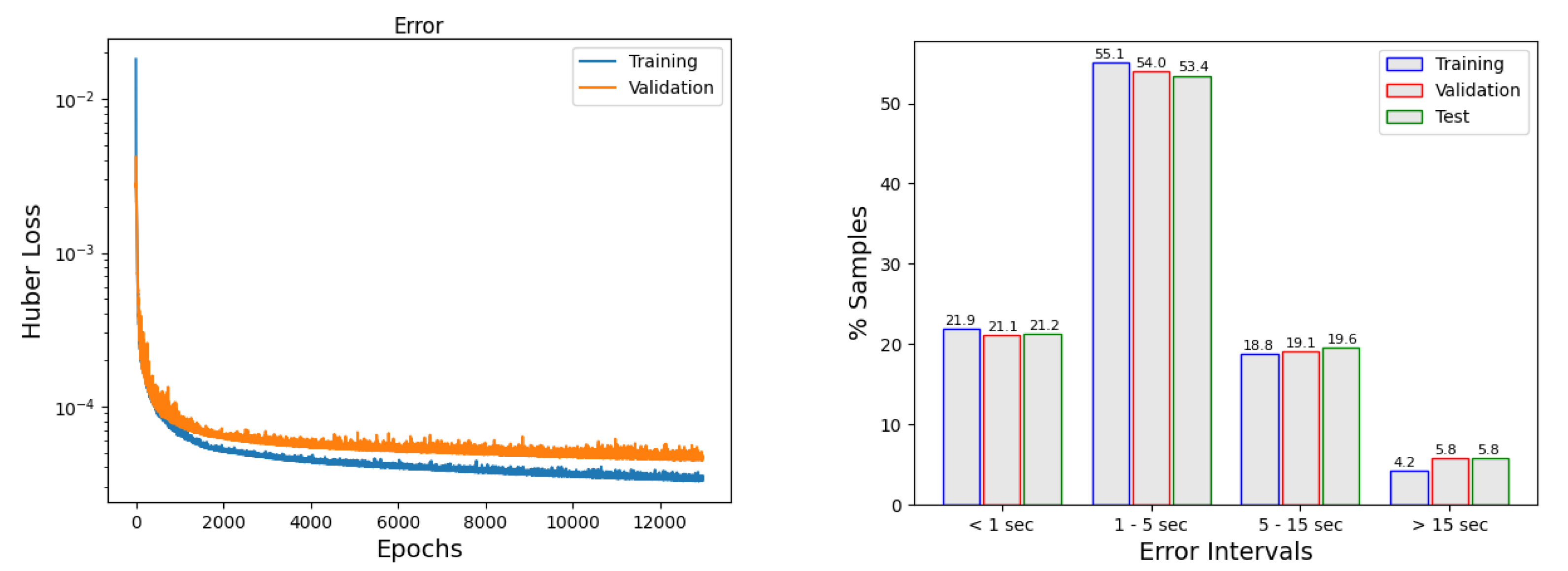
The left panel in
Figure 8 shows the evolution of the error as the model is trained. It can be observed how the callbacks are acting: The choice of the learning rate produces big jumps at the first part of the training and smaller variations occur when the number of epochs increase (larger than 2000). In addition, when the error is no longer decreasing, the
early stopping concludes the training. In general, to keep training, besides this point, does not necessarily improve the model. In
Figure 8, right panel, we can see how many of the predictions are in a given error interval.
Table 9 provides the results of the single neural network selected (model 23). It shows the absolute mean error and the absolute maximum error in each of the points and sets defined before. Very good results are obtained, with an average mean error of 0.38 cm for the test set at the six locations, and a maximum height error of 6.77 cm at Rota.
5.2. Ensemble Models for Maximum Heights
Once the single neural networks have been trained, combinations of several of them can be used to improve the results. We tried several combinations. Two different types of ensemble were attempted. One of them just performs a sampling of the space of possible solutions (weighted average MLP ensembles [
20]), and the other uses an optimization process, using any available information to make the next step in the search.
Table 10,
Table 11 and
Table 12 provide results of some possible combinations with two, three, and four models. In the column “Weights”, we round the weights associated with each model in the ensemble, and the column “Type” refers to the type of ensemble method used, space search or optimized search.
Several ensemble models combining five single models were tested, but in most cases, one of the weights associated with one particular single model was very close to 0, making this particular model contribution negligible.
As has been shown, several combinations for the ensembles were tried. Model 17 returns the best results, with an mean absolute error of 0.3 cm and a maximum error of 6 cm. This ensemble is composed of four models.
Table 13 and
Figure 9 allow us to compare the results obtained in this case with the single model selected before (
Table 9 and
Figure 8). Model performance was substantially improved.
5.3. Single Models for Arrival Times
In
Section 4, 17 NN models for the prediction of the arrival time of the tsunami wave were proposed, including the one to which we applied the regularization (see models in
Table 7 and
Table 8). The maximum error at estimating the arrival time ranged from 238.74 s for model 4 to 454.34 s for model 2. Errors in arrival times of about 5 min for an application to an early warning system are acceptable. As in the case of the maximum height prediction problem, the inputs were normalized to [0, 1].
Regarding the single model giving a smaller maximum error (model 4), it has six layers, five hidden layers, and the output layer. Each of the hidden layers has 100 neurons, and the hyperbolic tangent is used as activation function. The output layer has six neurons and no activation function. To reduce the mentioned overfitting from model 4, a soft L2 regularization on the weights was applied on the first layer. Additionally, a soft L2 regularization on the output was applied. The Adam optimizer was used with a initial learning rate of 0.001 (learning rate will be decaying with ReduceLROnPlateau callback). The batch size selected was 256, and the Huber loss function was used with . The output was normalized to [0.05, 0.95].
Two callbacks were applied. The early stopping, that stops the model when the minimum of the mean of the validation set predicted is not decreasing after 500 epochs, and the ReduceLROnPlateau, which reduces the learning rate if the validation loss has not been reduced in 180 epochs, multiplying by 0.75 each time and taking a minimum learning rate of 0.0001. It takes 12,975 epochs to train the NN.
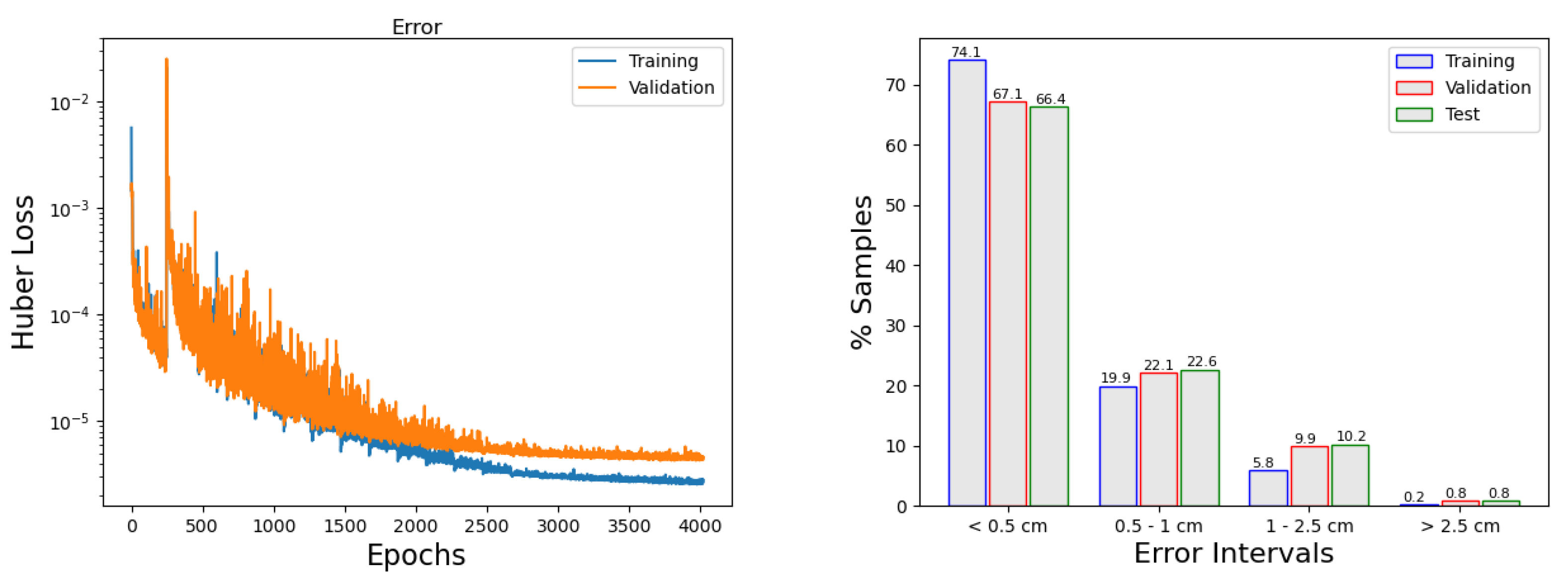
Figure 10 (left panel) shows the evolution of the error through the training process and how callbacks are acting. Similarly to what happened in
Figure 8, we can observe how the
early stopping ends the training when the criteria established above has been completed. In the right panel, the percentage of predictions within error intervals is depicted. It can be seen that most of the predictions (95.8% for training, 94.2% for validation, and 94.2% for the testing) have an error below 15 s, which is a very good result.
Table 14 provides the results for the reference single neural network (model 4 with the above-mentioned regularization). It shows the absolute mean error and the absolute maximum error in each of the six forecasting points and for the three datasets. Very good results are produced, with a mean error of 5 s and a maximum arrival time of 262 s.
5.4. Ensemble Models for Arrival Times
Once the 17 single neural networks were trained, combinations of them were tested in order to improve the results. As in the maximum height problem, weighted average MLP ensembles were used. In what follows, we denote as model 17 the one obtained from model 4 after regularization.
Table 15,
Table 16 and
Table 17 show the results of some possible combinations using two, three, and four single models.
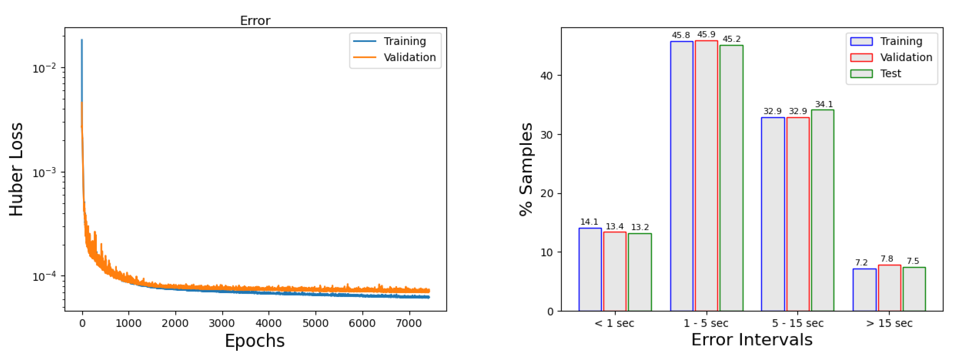
With ensemble techniques, we considered 18 additional models (see
Table 15,
Table 16 and
Table 17). Among them, we retain ensemble model 7 in
Table 15, as it is the one with a smaller mean absolute error (3.90 s) and with a maximum error of 212 s (see
Table 18). This ensemble is composed of the contribution of two single models, models 4 and 17.
Table 18 presents the results for the ensemble model 7, which can be compared with the single model results in
Table 14. Very good results are obtained, with a mean error smaller than 4 s and a maximum arrival time of 212 s.
Figure 11 shows the percentage of predictions within error intervals. It can be seen that most of the predictions (97.8% for training, 96.0% for validation, and 96.2% for the testing) have an error below 15 s, which is a very good result and improves single model results.
6. Towards a TEWS Based on NN Models
The aim of this work is to present a methodological approach that can be used to construct a TEWS based on NN models. The basic building blocks of such a system are described here, in particular NN models for the maximal height forecast and arrival time estimation at a set of forecast points. To have a complete TEW system, for example, on the Atlantic coast of southeastern Spain (Huelva and Cádiz provinces), two extensions must be considered. First, it is necessary to cover the whole coast with forecast points. To do so, our experience leads us to propose a mixed strategy consisting of increasing the number of forecast points in the models we have developed in this paper, on the one hand, and on the other, dividing the coast into segments and training different models on each of these segments. To test the performance of models with more forecast points in a single segment, we will here use 12 points instead of 6 for the CA01 coastal segment. The same set of numerical simulations used to train the six-point models presented in previous sections will be used now to train the 12-point models. An example of this will be described below and the results presented in the Annex. As long as the number of forecast points is not too large, this approach can provide good results; of course, the price to pay is a decrease in performance when the number of forecast points is increased. The second extension required to have a complete TEWS is to train an NN model for every single potential tsunamigenic source in the area of interest (in our case, in the Northeastern Atlantic area). More specifically, for each active fault, a model with forecast points at each of the segments defined in the coastal stripe (in our case for HU01, HU02, CA01, CA02, and CA03) must be trained.
Finally, we are trying to assess the performance of NN models similar to the two single models that we have retained as reference in previous sections, one for maximum height and another for arrival time, but now trained to output forecasts in 12 instead of in 6 locations. With these 12 points, we could have a coverage of the coastal segment CA01 dense enough for the purpose of a TEWS. Using the same dataset of simulations used to generate all the NN models described in the present study, we trained the two single models with 12 forecasting points for maximum heights and arrival times, and the results obtained are presented in the Annex.
7. Conclusions
In recent years, tsunami simulation codes have been developed and improved, returning very accurate results in progressively reduced computing times. Nevertheless, the use in TEWS requires extremely short computing times, not possible yet if high resolution or inundation must be computed. To solve this problem, in this paper, we have proposed the use of deep learning techniques to predict the maximum height and the arrival time to six forecasting points in the coast of Cádiz, using the Horseshoe fault as generating fault.
For each of these two problems, we developed single models and combined some of them to obtain ensemble models that improved the results. The results obtained confirm that deep learning is a useful tool to predict the maximum height and the arrival time of a tsunami at several offshore points near the coast.
As summary:
The maximum heights obtained by the simulations reach values between 0.21 m and 3.47 m, and the arrival time oscillates between 2565 s and 5504 s.
The mean absolute error we obtained with a single model for tsunami height is 0.38 cm and the maximum error is 6.77 cm.
Most of the samples are under 2.5 cm of absolute error for the maximum height.
Ensemble techniques improve the performance of the results, reducing the maximum error to 6 cm.
The mean absolute error we obtained with a single model for tsunami arrival times is 5 s and the maximum error is 262 s.
Most of the samples are under 15 s of absolute error for the arrival time.
Ensemble techniques improve the performance of the results, reducing the maximum error to 212 s.
The results presented are promising: the estimations at the forecast points provided by the NN models developed are accurate with small errors. The outputs of these models can serve to generate alert levels, which is the final aim of a TEWS, along the coast. To do so, only a few points per coastal segment are required. This justifies the development of six-point models for each coastal segment. Nevertheless, we also generated 12-point models, and the results obtained are presented in the
Appendix A. This was performed using the same dataset of numerical simulations. As long as the number of forecast points is not too large, the resulting models also provide good results, although (and obviously) with decreasing performance as the number of points increases.
The next step on the way to have a complete TEWS in this region is to train NN models for assessing maximum heights and arrival times for this same segment, CA01, but for all the potential seismic sources in the area. This means performing on the order of 16,000 numerical simulations for each active fault with the potential of generating tsunamis with impact in the selected coast. Then, and finally, the same process must be repeated for the other four areas defined by the Spanish TEWS in the Atlantic coast of Andalucia, in particular for H01, H02 for Huelva and CA02, CA03 for Cádiz (see
Figure 1).
Finally, the results of this study can be extended to other tsunami forecasting problems. For example, the use of convolutional neural networks or recurrent neural networks to simulate the inundated area, or the use of physically informed neural networks (PINNs) to increase the complexity of the physical model (dispersive or non-hydrostatic models).


 ,
, 


