Status of Mean Sea Level Rise around the USA (2020)


Coastal Education and Research Foundation, Coconut Creek, FL 33073, USA
GeoHazards 2021, 2(2), 80-100; https://doi.org/10.3390/geohazards2020005
Submission received: 23 March 2021
/
Revised: 5 May 2021
/
Accepted: 13 May 2021
/
Published: 19 May 2021
Abstract
:The potential threats to the USA from current and projected sea level rise are significant, with profound environmental, social and economic consequences. This current study continues the refinement and improvement in analysis techniques for sea level research beyond the Fourth US National Climate Assessment (NCA4) report by incorporating further advancements in the time series analysis of long tide gauge records integrated with an improved vertical land motion (VLM) assessment. This analysis has also been synthesised with an updated regional assessment of satellite altimetry trends in the sea margins fringing the USA. Coastal margins more vulnerable to the threats posed by rising sea levels are those in which subsidence is prevalent, higher satellite altimetry trends are evident and higher ‘geocentric’ velocities in mean sea level are being observed. The evidence from this study highlights key spatial features emerging in 2020, which highlight the northern foreshore of the Gulf Coast and along the east coast of the USA south of the Chesapeake Bay region being more exposed to the range of factors exacerbating threats from sea level rise than other coastlines at present. The findings in this study complement and extend sea level research beyond NCA4 to 2020.
1. Introduction
Climate change has become one of the biggest threats facing mankind during the course of the 21st century and beyond. The associated social, environmental and economic implications are unparalleled within the context of a global population expected to increase by 2 billion persons in the next 30 years, and which could peak at nearly 11 billion by around 2100 [1]. Mean sea levels, greenhouse gas concentrations and temperatures are the key proxy indicators by which climate change is generally monitored and quantitatively measured. The threats associated with a rising mean sea level are most acute within the low elevation coastal zone (LECZ), defined globally as a geographical land margin connected to the coast, less than 10 m above sea level [2,3].
Fleming et al. [4] note that America’s trillion-dollar coastal property market and public infrastructure are threatened by the ongoing increase in the frequency, depth and extent of tidal flooding due to sea level rise, with cascading impacts on the larger economy. By 2014, some 42% of the US population (or approximately 134 million people) resided in coastal shoreline counties [5]. Within shoreline counties of the US, it has been estimated that housing stock and commercial businesses worth at least USD 1.4 trillion sit within approximately 200 m of the coast [6]. The NCA4 report [7,8,9] also notes that in addition to threats to property and infrastructure, projected sea level rise will significantly affect diverse ecosystems such as beaches, intertidal zones, reefs, seagrasses, salt marshes, estuaries and deltas that support a range of important services including fisheries, recreation and coastal storm protection [4].
The prominence of the climate change issue has placed more emphasis on examination of the extensive global repository of relative mean sea level records [10,11] and more recent satellite altimetry data covering the global oceans (post 1992). Satellite altimetry, space gravity and Argo measurements have provided unprecedented insight into the magnitude, spatial variability and causes of present-day sea level change during the altimetry era [12,13,14,15,16,17].
The literature is replete with mean sea level research being conducted at increasingly finer spatial scales seeking to understand key temporal changes and signatures to assist with scientific understanding of the phenomena to better inform the development of strategic planning and adaptation endeavours.
The United States contains one of the best networks of long tide gauge records anywhere in the world, with quality-controlled records available from the Permanent Service for Mean Sea Level (PSMSL) [10,11] extending back to 1854 (San Francisco), with some 15 records exceeding 100 years in length. There are numerous active records around the USA longer than 75 years in length, which are considered to have sufficient length for analysis of trends and accelerations in mean sea level [18,19,20].
Whilst longer tide gauge records permit the means to detect fundamental changes in records over time (e.g., the rate of mean sea level), Watson and Lim [21] note that difficulties frequently arise in using such records to understand mean sea level. This is because tide gauges record all physical processes causing the water level to change, including but not limited to: melting of snow and ice reserves and thermosteric sea level change (resulting from climate change), dynamic climate mode (and other) influences and vertical land motions (VLM) at the tide gauge. Isolating the influence of these differing physical processes from tide gauge records provides the means to improve our understanding of mean sea level rise at increasingly localised scales from these long tide gauge records.
Singular Spectrum Analysis (SSA) is a powerful data analysis tool which permits separating signals from a time series record into elements of trend (in this case, a slowly varying climate change signal), dynamic components and noise, providing significant appeal for environmental data. Extensive time series analysis testing has determined that data adaptive spectral techniques such as one-dimensional SSA provide greater utility in isolating the ‘trend’ component with improved temporal precision for long time gauge records [22]. Over recent years, this analysis tool has been optimised for the benefit of sea level research [20,23,24], enabling improved resolution of the mean sea level signal.
This current study continues the refinement and improvement in analysis techniques for sea level research beyond the NCA4 report [7,8,9], incorporating advancements in the time series analysis of long tide gauge records [20,21,23,25] with improved integration of vertical land motion (VLM) assessment [26]. This analysis has also been synthesised with an updated regional assessment of satellite altimetry trends in the sea margins fringing the United States.
2. Materials and Methods
The methods used in this study are consistent with those broadly established in more recent published regional sea level assessments [21,23], which build on the extensive testing and analysis for long tide gauge record assessment [20]. The following sections summarise these methods. The ‘TrendSLR’ [24] extension package within the open-source framework of the R Project for Statistical Computing [27] contains both analysis and spectral diagnostic tools used to undertake key elements of the analysis.
2.1. Data Sources Used in the Study
Annual and monthly average water level data were obtained from the PSMSL [10,11] for the analysis. Where necessary, additional data to extend relevant time series to the end of 2020 have been sourced directly from the National Ocean Service, National Oceanic and Atmospheric Administration (NOS NOAA) [28]. In total, 92 stations records were available spanning the satellite altimetry era (post 1992) around the United States. Of these records, 39 exceeded 75 years in length and were deemed suitable for long-term trend analysis. Each record has been assigned a station ID beginning with Nawiliwili Bay, Hawaii (ID = 1) in the central Pacific Ocean, progressing around the Hawaiian Islands, then east to west along the Alaskan coastline, south along the west coast of the USA, east along the Gulf of Mexico and then north along the east coast of the USA to Eastport, Maine (ID = 92) in the Bay of Fundy (refer Figure 1, Table 1).
Sea Surface Height Anomaly (SSHA) altimeter products have been sourced from the European Commission’s Copernicus Marine Environment Monitoring Service (CMEMS) [29]. The two-satellite merged global gridded L4 (008_057) product is provided with a daily temporal resolution on a spatial density of 0.25° × 0.25° (Cartesian). These time series data permit VLM estimation at each tide gauge location based on trends from differenced altimetry–tide gauge (ALT-TG) techniques. Refer to this section for further details.
In addition to the gridded altimetry product above, trends of SSHA spanning the period September 1992 to October 2019 are available for the sea margins around the USA and distributed by Archiving, Validation and Interpretation of Satellite Oceanographic (AVISO) [30]. These gridded linear trends have been used to assess spatial signatures of sea level rise and are provided with no correction for Glacial Isostatic Adjustment (GIA).
2.2. Historical Tide Gauge Analysis
The trend analysis applied to annual average time series data is based on similar detailed regional sea level studies conducted around the United States, Europe, the Republic of Korea and Australia [21,23,31,32] utilising the capability of SSA to separate out the slowly varying climate change signal from the time series record. SSA does this by amplifying the signal-to-noise ratio by separating the original time series into low-frequency trends and narrow-band quasi-periodic signals, with the rest (assumed to be noise) distributed among the filters [33]. Through use of an embedding dimension, the original time series is projected via a series of lagged copies of the original time series into the form of what is referred to as a trajectory matrix. Singular value decomposition (SVD) functions can then be performed on the matrix to resolve individual components in order of rank of contribution to the time series from trend and oscillatory signals all the way down to dimensionless noise. The applied methodology has been slightly updated and refined after Watson (2016, 2017, 2018) [20,31,32] to incorporate the findings of Mann, Steinman and Miller (2020) [34] regarding the approximate cutoff between trend and dynamic (or oscillatory) behaviour associated with the climate system. The specifics are described in more detail in Step 2 (Section 2.3) below.
Trend analysis has been performed only on records in the PSMSL longer than 75 years based on established principles in the literature [18,19,20] (refer to Table 1 for details). Various records exceeding 75 years in length (Hilo, Adak Sweeper Cove, Seward, Yakutat, Skagway, Santa Monica and Lewes) all contained significant portions of missing data that were not able to be satisfactorily filled (refer to Step 1 for details). Although there were significant portions of missing data in the New York and Fernandina Beach records, residual portions from 1893 and 1939, respectively, exceeded 75 years in length and were therefore sufficient to undertake trend analysis with small gaps readily filled within desired limits. A total of 39 records were able to be considered for trend analysis.
Gaps in environmental records such as long tide gauge records are quite common, requiring consideration in terms of trend analysis. The use of SSA requires complete time series; therefore, gap-filling has been undertaken where necessary. However, limits have been imposed on the extent of gap-filling to preserve the integrity of the original record and limit the potential for influencing trend determination. Testing and analysis of gap-filling for sea level records has been previously undertaken [20] and the recommendations of this work have been applied in this study. Broadly, these recommendations suggest filling of records only where the total gaps are less than 15% of the time series and the largest continuous gap is no larger than 5%.
2.3. Step by Step Methodology
The methodology applied in analysing the observational tide gauge records can be broadly summarised in the following six steps.
Step 1: Gap-filling of tide gauge records. As discussed previously, gap-filling must be undertaken to permit SSA decomposition for trend analysis. The ‘TrendSLR’ package contains various gap-filling functions suitable for annual average tide gauge records. The first preference has been to use an iterative SSA procedure [35,36] which fills gaps based on the dominant spectral properties of the continuous sections of the original time series. However, on the limited occasions where the spacing of the gaps or complexity of the residual time series structure does not permit the iterative SSA procedure to converge within prescribed tolerance limits [36], alternative options available in the ‘TrendSLR’ package have been used to fill gaps including weighted moving average and Stineman interpolation [37]. The gap-filling functions in the ‘TrendSLR’ package permit visual inspection to optimise the filling method and check that artificially generated gaps appear reasonable within the context of the time series.
Step 2: Estimation of ‘relative’ mean sea level. Specifically, this study uses the basic one-dimensional version of SSA proposed by Bromhead and King (1986) [38] built into the ‘Rssa’ extension package in R [36] to decompose the annual average mean sea level time series to isolate ‘relative’ mean sea level (in this case, a slowly varying trend), from the more dynamic components and noise.
A key SSA parameter is the embedding dimension (or ‘window’, as it is commonly referred to). The embedding dimension is recommended in the range of one-quarter to one-half the length of the time series with one-half the maximum possible [33,39,40]. Selecting the maximum range ensures optimal possible separability between the resolved components from the SSA decomposition. Given that the imperative of the exercise is to isolate mean sea level (or trend) with improved temporal resolution, it is strongly recommended to use the maximum embedding dimension afforded by the data record to optimise the separability of resolved components and minimise mixing across signals [33]. This recommendation has been observed for this study.
‘Relative’ mean sea level can then be estimated by aggregating the components from the SSA decomposition which exhibit ‘trend-like’ characteristics. This can be done automatically using techniques such as frequency thresholding [41], which operates on the spectral properties of individual components from the SSA decomposition. The published findings of Mann, Steinman and Miller [34] indicate that, from extensive climate research, the difference between trend and dynamic (or oscillatory) behaviour appears to reside around the 50 year period (or the frequency band of 0.02 cycles per year).
For this study, ‘relative’ mean sea level has been estimated using frequency thresholding to aggregate components from the SSA decomposition in which more than 50% of the relative spectral energy is evident in the low-frequency band between zero and 0.02 cycles per year to accord with the findings of Mann, Steinman and Miller [34].
Step 3: Estimation of ‘relative’ mean sea level velocity. A fitted cubic smoothing spline model permits estimation of the time varying velocity of the estimated ‘relative’ mean sea level determined from Step 2. Extensive testing of fitted smoothing splines for mean sea level research [20] recommends the general application of 1 degree of freedom (DOF) for every 8 years of record when fitting a spline for this purpose. The ‘TrendSLR’ package permits visualisation of the fitted spline and fine tuning of the DOF if deemed necessary.
Step 4: Estimation of standard errors associated with analysis of individual tide gauge records. This process involves several steps, the first being to remove the serial correlation in the residuals between the ‘relative’ mean sea level estimate (Step 2) and the original time series. This is achieved by fitting a standard autoregressive integrated moving average (or ARIMA) time series model. This step is undertaken automatically by the ‘TrendSLR’ package via Hyndman and Khandakar’s stepwise algorithm [42].
Errors in the estimation of ‘relative’ mean sea level and the associated velocity are then determined through bootstrapping techniques. Steps 2 and 3 are repeated 10,000 times by randomly recycling the uncorrelated residuals. With 10,000 generated ‘relative’ mean sea level and associated velocity time series, standard deviations are readily estimated for both sets of outputs at each time step.
Step 5: Estimation of VLM at tide gauge record. VLM has been estimated using an ALT-TG technique initially proposed by Ostanciaux et al. [43] and recently revised and updated by Watson [26] using standard gridded altimetry products. In essence, the approach is based on linear regression of the difference between monthly average SSHA (altimetry derived) and the ‘relative’ tide gauge record. Standard errors are automatically generated from the least squares fitted model.
From a global analysis of ALT-TG and continuous GPS measurements, Watson [26] determined that ALT-TG VLM estimates were improved by using standard gridded altimetry SSHA products closest to the tide gauge but no closer than 30 km from the open coast and islands. CMEMS [29] daily SSHA data have been converted into monthly average time series spanning January 1993 to February 2020. Monthly average tide gauge data have been used for the ALT-TG analysis spanning the same timeframe.
Step 6: Correction of ‘relative’ mean sea level velocity to ‘geocentric’ reference frame for each tide gauge record. The VLM (Step 5) is added to the ‘relative’ velocity (Step 3) to estimate velocity in a ‘geocentric’ reference frame.
3. Results
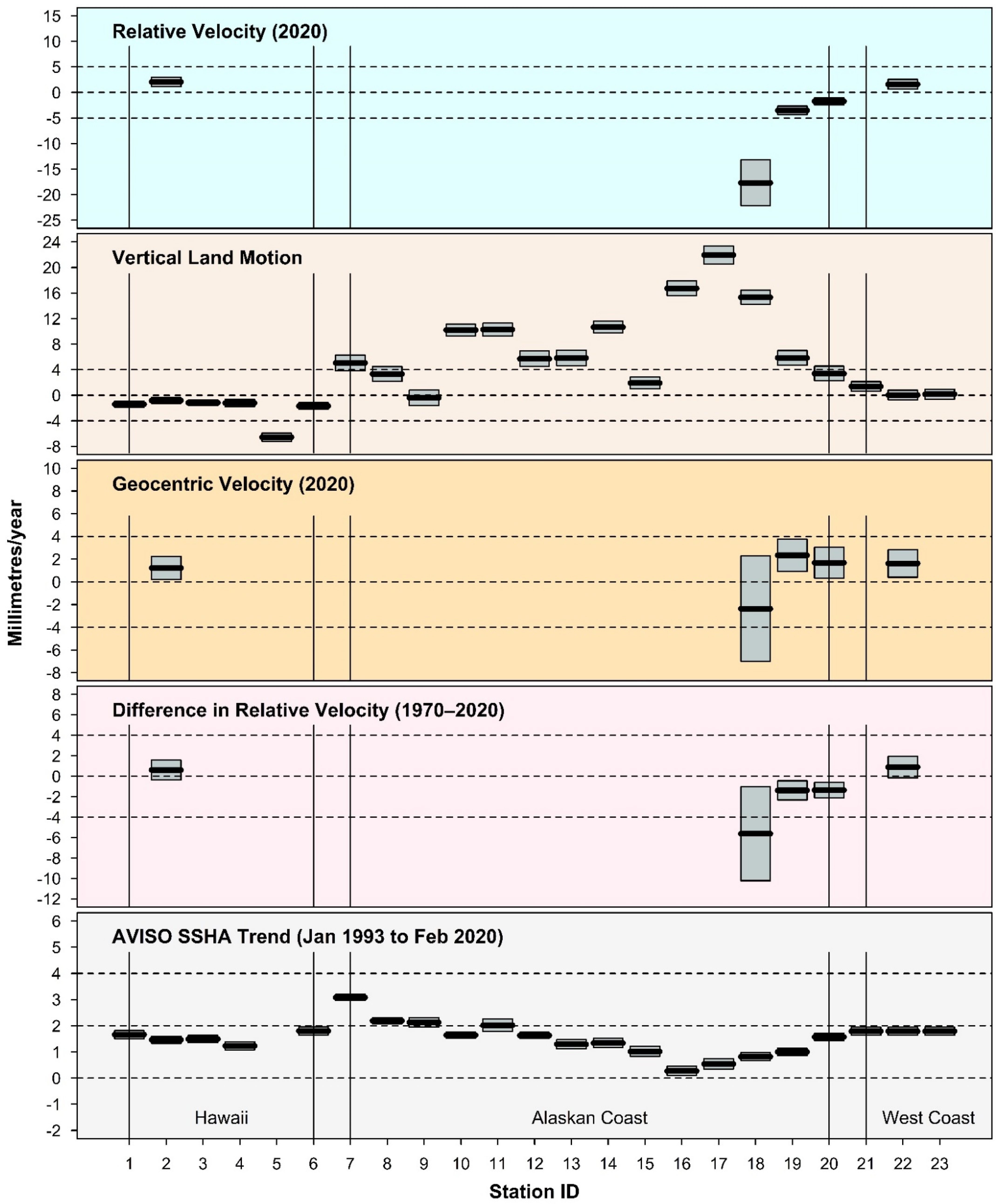
Importantly, all analysis results presented include error margins at the 95% confidence level (CL), unless noted otherwise. Key results have been presented diagrammatically for each of the 92 stations analysed around the coastlines of the USA (refer to Figure 2, Figure 3, Figure 4 and Figure 5). The 39 records were sufficiently long to undertake trend analysis and permit detailed temporal and spatial signatures of changes in mean sea level to be identified. The ‘relative’ mean sea level analysis is largely dominated by local VLM processes whereas the ‘geocentric’ mean sea level analysis reflects more strongly the direct signature of climate change phenomena.
3.1. ‘Relative’ Mean Sea Level Velocity
From the ‘relative’ mean sea level velocity analysis in 2020, clear spatial patterns are apparent for how the rate of mean sea level is perceived standing on the land. Along the Alaskan coast, the uplifting of the land mass associated with the unloading from the retreat of the Laurentide ice sheet across North America is clear. For example, the mean sea level velocity at Juneau (ID = 18), inside the Stephens Passage (Alaska), is estimated at −17.7 ± 2.3 mm/year—that is, in 2020, the apparent sea level is falling relative to the land at high rate. By comparison, as the influence of the strong post-glacial rebound (PGR) signature moderates, moving further south along the west coast of the USA, the ‘relative’ velocity in 2020 flips from negative to positive between San Francisco (ID = 37) and San Diego (ID = 44). Along the coastline of the Gulf of Mexico between Texas and Florida, ‘relative’ velocities in mean sea level reside at or above 5 mm/year in 2020 (average = 6.3 mm/year). These increased velocities are driven by a combination of persistent subsidence along this coastal sector and elevated SSHA trends within the Gulf of Mexico attributed to climate change. The peak ‘relative’ velocity in 2020 of 9.8 ± 1.3 mm/year was observed at Galveston, Texas (ID = 47).
For context, the average rate of sea level rise forecast for the last 5 years of the 21st century by the Intergovernmental Panel on Climate Change (IPCC) under Representative Concentration Pathways (RCP) 4.4 and 8.5 are of the order of 7 (range 4–9) and 15 (range 10–20) mm/year, respectively [44]. The corresponding amount of global mean sea level rise to 2100 for RCP4.5 and 8.5, relative to 1990, is of the order of 549 (range 385–724) and 842 (range 609–1105) mm [44].
Along the east coast between Florida and New York, the average ‘relative’ rate of mean sea level rise in 2020 is around 4.7 mm/year, moderating northwards between New York and Eastport at an average rate of less than 3 mm/year.
3.2. Vertical Land Motions
The analysis reveals spatially dominant patterns of vertical land motion around the coastlines of the USA that have important implications regarding the threat posed by rising sea levels. In particular, where land margins are rising (or uplifting), the threat of increasing sea levels is moderated, but where trends of land subsidence prevail, the ‘relative’ rate of submergence from a rising ocean will be exacerbated.
The strong PGR signal associated with uplifting of the retreating Laurentide ice sheet is evident along the Alaskan coastline, where a range of stations exhibit rates of uplift exceeding 10 mm/year (Kodiak Island, Seldovia, Valdez, Yakutat, Skagway and Juneau). Skagway measures the highest rate of uplift at around 22 mm/year. If these rates of uplift are sustained, much of the Alaskan coastline will remain largely unaffected by even the higher range of projected global sea level rise (e.g., RCP8.5) throughout the 21st century. Although the PGR influence moderates along the coast southward of Alaska, several stations along the west coast in the states of Washington (Cherry Point, Port Angeles, Neah Bay and Toke Point), Oregon (Astoria, Port Orford) and California (Crescent City) exhibit rates of uplift exceeding 1 mm/year. Moving south of Crescent City though, between Humboldt Bay and San Diego, the trend of VLM over the 12 stations in this coastal sector flips over to subsidence, averaging around −1.3 mm/year. This trend also persists around the Hawaiian Islands, with 4 of the 6 stations exhibiting subsidence exceeding 1 mm/year.
The northern foreshore of the Gulf of Mexico and along the east coast USA are dominated by subsidence, but from various contributory factors. The subsidence along the foreshores of the Gulf of Mexico has been driven ostensibly by a range of factors which include compaction of sediments due to increased urbanisation in marshland areas [45] and aquifer system compaction due to extensive groundwater withdrawal [46,47]. The influence of GIA processes along this sector of coastline is comparatively small [46]. From the 15 stations between Port Isabel, Texas and Vaca Key, Florida, the average rate of subsidence is around −2.4 mm/year. However, over the 750 km section of coast between Rockport, Texas and Grand Isle, Louisiana, the rate of subsidence increases to an average rate of −4.9 mm/year, resulting from the extensive groundwater withdrawal programs from the primary aquifers comprising the Gulf Coast aquifer system (the Chicot, Evangeline and Jasper aquifers) [47].
Along the east coast of the USA, subsidence dominates, averaging −1.7 mm/year from 33 stations between Fernandina Beach, Florida and Eastport, Maine. However, GIA processes dominate over other contributory subsidence processes along sectors of the east coast caused by ongoing relaxation of the peripheral forebulge associated with the last deglaciation of the Laurentide ice sheet [48,49].
Quite distinct from the PGR being experienced along the Alaskan coast by the former magnitude of the Laurentide ice sheet, along the east coast of the USA, the location and scale of the ice sheet levered the land upwards. Following the retreat of the ice sheet and subsequent collapse of the peripheral forebulge, the maximum subsidence experienced occurs just south of the maximum glacier extent [49]. It is suggested that these stronger signatures of subsidence owing to these processes would be expected to occur near North Carolina, Maryland and Virginia [48]. Some 11 of the 33 east coast stations considered indicated rates of subsidence exceeding 2 mm/year, with three sites (Lewisetta, Virginia; Lewes, Delaware; and Cape May, New Jersey) exceeding 3 mm/year.
3.3. ‘Geocentric’ Mean Sea Level Velocity
Having corrected ‘relative’ mean sea level velocity in 2020 for VLM, clear spatial patterns in mean sea level velocity are apparent when considered from a ‘geocentric’ (or fixed) reference datum. These spatial patterns are ostensibly climate change fingerprints resulting from increases in the mass of the ocean driven by melting of snow and ice reserves and thermal expansion of the ocean water mass. ‘Geocentric’ velocities in 2020 can also be readily compared to the current rate of global mean sea level rise estimated at 3.6 ± 0.4 mm/year over the period 2006–2015 [44].
The ‘geocentric’ rate of mean sea level in 2020 at the Hawaiian Islands is estimated at 1.2 ± 1.0 mm/year (Honolulu). This velocity is comparable to the average ‘geocentric’ velocity in 2020 from the 11 stations along the west coast of the USA at 1.5 mm/year. However, within this sector of coastline, the stations north of Monterey, California average around 2.0 mm/year compared to those further to the south (between Port San Luis and San Diego), which average a mere 0.5 mm/year.
Along the northern foreshore of the Gulf Coast, the average ‘geocentric’ velocity in 2020 is much higher at 4.0 mm/year, with Key West, Florida and Galveston, Texas recording the second and third highest ‘geocentric’ velocity in 2020 around the USA at 5.5 ± 1.7 mm/year and 5.3 ± 1.3 mm/year, respectively.
The east coast of the USA presents a slightly different picture, with the average ‘geocentric’ velocity in 2020 from 19 stations records equating to 2.4 mm/year. There would appear to be a point of distinction along the east coast around Chesapeake Bay. For nine stations between Fernandina Beach, Florida, and Chesapeake Bay (inclusive), the average ‘geocentric’ velocity in 2020 is around 3.2 mm/year compared to the 10 records further north to Eastport, Maine, which average just under 1.8 mm/year. The highest ‘geocentric’ velocity across the USA was estimated at 6.0 ± 1.5 mm/year in 2020 at Baltimore, Maryland.
3.4. Acceleration in Mean Sea Level from 1970 to 2020
The analysis techniques in this paper permit the time varying velocity in mean sea level to be estimated at each year of the record as part of the longer-term trend analysis (see Section 2). By considering the difference in the ‘relative’ velocity in mean sea level between 1970 and 2020, one can detect whether (or not) the velocity is increasing over the past 50 years. If the velocity is increasing, an acceleration must be present in order to do so.
Similarly, distinct spatial features are evident from this analysis. From the records along the west coast USA, including Hawaii (but excluding Alaskan stations owing to large PGR effects), the average increase in ‘relative’ velocity in mean sea level over this timeframe from 11 stations records is 0.7 ± 1.5 mm/year, which, although positive, is not statistically different from zero at the 95% CL. From these records, only the Almeda, California record indicates a statistically significant increase in velocity (acceleration) over the past 50 years at 1.6 ± 1.4 mm/year.
However, for the five stations around the northern foreshore of the Gulf Coast, the average increase in ‘relative’ velocity in mean sea level over this timeframe is 2.7 ± 2.2 mm/year, representing a statistically significant acceleration. Further, each station record in the Gulf separately exhibits a statistically significant acceleration.
Along the east coast USA, spatial patterns mirror those associated with the results of the ‘geocentric’ velocity analysis (Section 3.3). The average increase in ‘relative’ velocity in mean sea level over this timeframe from 19 stations records along the east coast is 1.3 ± 1.6 mm/year, which, although positive, is not statistically different from zero at the 95% CL. However, from the nine stations between Fernandina Beach, Florida, and Chesapeake Bay (inclusive), the average increase in ‘relative’ velocity in mean sea level over this timeframe is 1.8 ± 1.4 mm/year, representing a statistically significant acceleration, with all stations except Washington DC and Sewells Point, Virginia separately exhibiting a statistically significant acceleration. This contrasts to the 10 stations further north between Atlantic City, New Jersey and Eastport, Maine, where the average increase in ‘relative’ velocity in mean sea level over the last 50 years is only 0.8 ± 1.8 mm/year, which, although positive, is not dissimilar from the results for the west coast stations (0.7 ± 1.5 mm/year) and not statistically different from zero at the 95% CL.
3.5. Sea Surface Height Trends from Satellite Altimetry
Trends in SSHA observed from multi-mission satellite altimetry data over the period from September 1992 to October 2019 made available by AVISO data [30] show some key spatial signatures both around the coastline and in the adjoining sea margins around the USA. It should be clearly emphasised here that these are linear trends in SSHA over the 27.1-year altimetry period, which will be significantly influenced by internal climate mode forcings (such as ENSO, etc.) on such timescales. These trends are therefore not directly comparable to ‘relative’ and ‘geocentric’ velocities determined from the longer tide gauge record analysis in this study, which firstly remove such influences from the record and secondly estimate time varying velocities in real time, rather than averages across the record length.
Notwithstanding, from the analysis of gridded products nearest the tide gauge sites no closer than 30 km from the open coast and around islands, the average trend across all 92 locations was approximately 2.5 mm/year, nearly 1.1 mm/year lower than the current rate of global mean sea level rise estimated at 3.6 ± 0.4 mm/year over the period 2006–2015 [44].
From the 44 stations comprising the Hawaiian Islands, Alaskan and east coast stations, the average SSHA trend is 1.5 mm/year. However, for the 11 locations analysed around the northern foreshore of the Gulf Coast between Port Isabel, Texas and Vaca Key, Florida, the SSHA trend averages 4 mm/year. The highest trend along the foreshores around the USA was 4.4 mm/year at Cedar Key, Florida. High rates of trend persist north from Florida along the east coast USA moderating below 3 mm/year to the north of Chesapeake Bay.
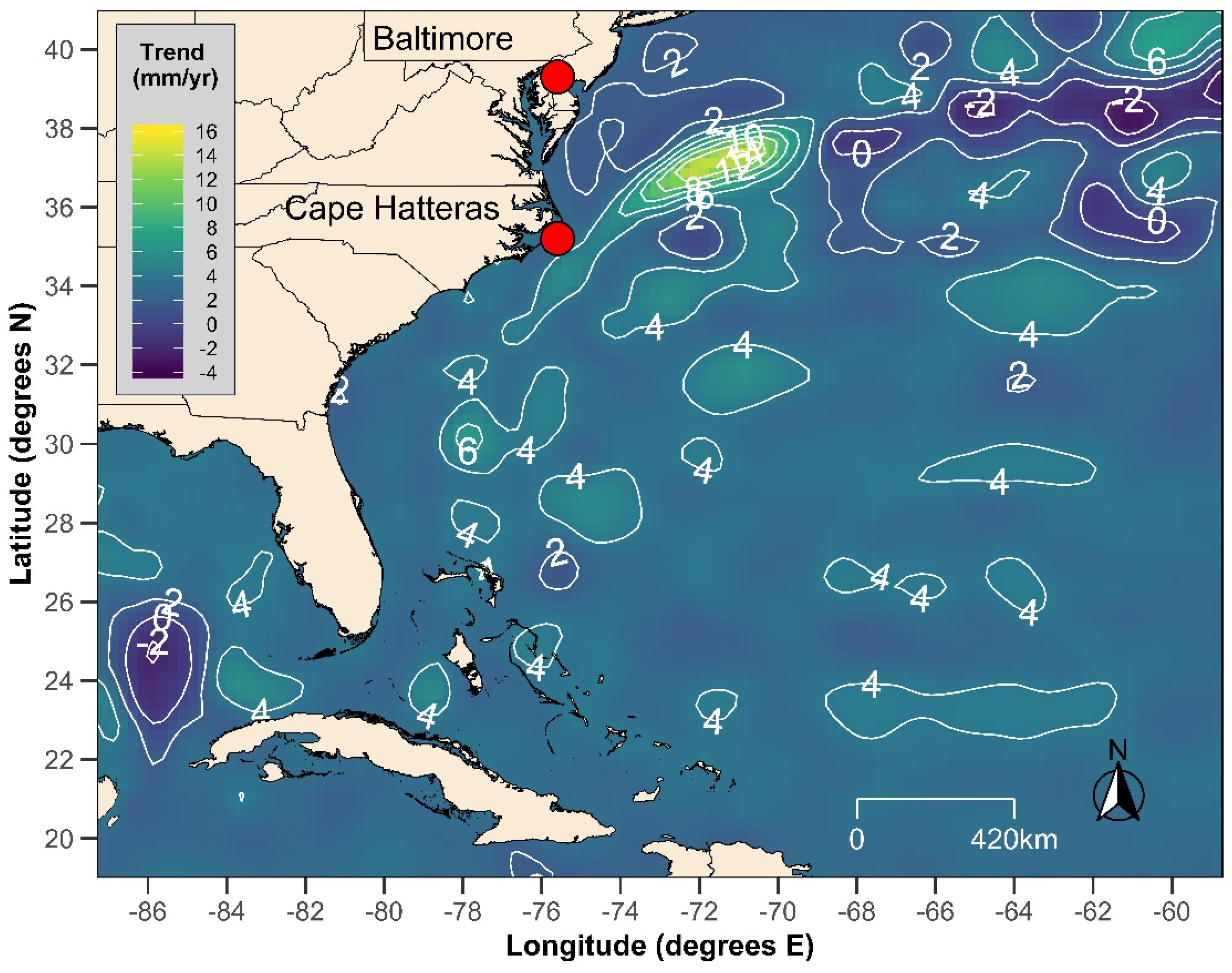
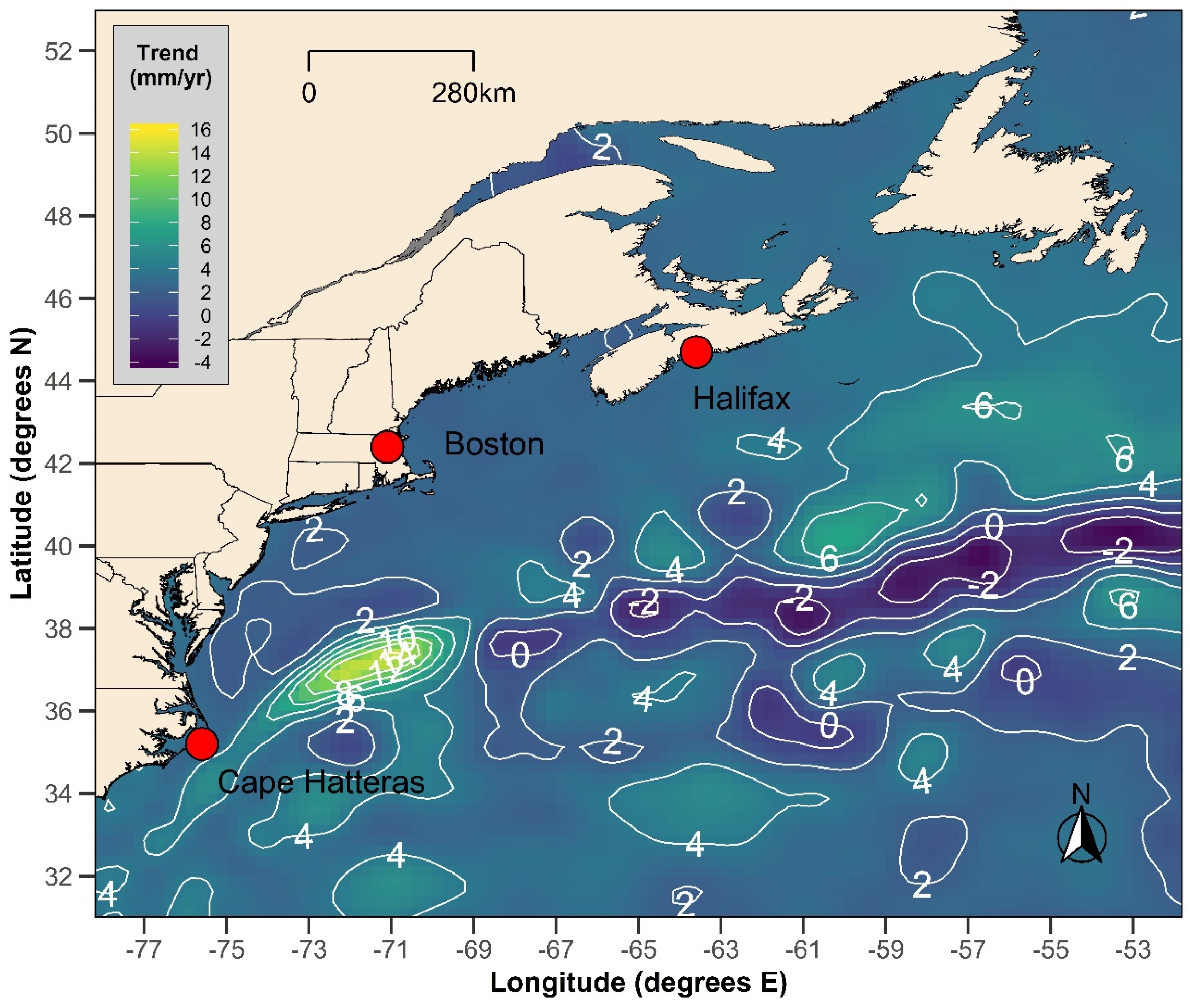
The altimetry SSHA trend analysis highlights large spatial variations in the sea margins around the USA (Figure 6). From this region, specific margins of interest are further highlighted in Panels 1–4 in the corresponding Figure 7, Figure 8, Figure 9 and Figure 10. From the overall perspective (Figure 6), the average of the 113,383 gridded SSHA trends for the period from September 1992 to October 2019 is 2.5 mm/year. Only 14% of the grid points depicted indicated a trend above the current rate of global mean sea level rise estimated at 3.6 ± 0.4 mm/year over the period 2006–2015 [44]. The highest trend of 14.4 mm/year was observed in the North Atlantic Ocean along the northern edge of the Gulf Stream off the east coast of the USA at −70.875° E and 37.375° N. Conversely, the lowest trend of −4.2 mm/year was located further east, similarly within the influence of the Gulf Stream at −44.375° E and 41.875° N.
Panel 1 delineates the SSHA trends in the North Pacific Ocean within the vicinity of the west coast of the USA (Figure 7), indicating an average from 8321 gridded SSHA trends of only 1.8 mm/year. The highest trend observed within Panel 1 was 4.7 mm/year at −114.125° E and 29.875° N within the Delfin Basin of the Gulf of California.
Conversely, the lowest trend of −0.9 mm/year was located at −123.375° E and 32.875° N, approximately 450 km west of the coastline from Los Angeles. Less than 1% of the grid points depicted in Panel 1 indicated a trend above the current rate of global mean sea level rise.
Panel 2 delineates the SSHA trends in the Gulf of Mexico and Straits of Florida (Figure 8), indicating an average from 3604 gridded SSHA trends of 3.3 mm/year. The highest trend observed within Panel 2 was 6.1 mm/year at −90.125° E and 27.125° N, approximately 200 km due south of the Mississippi Delta. Conversely, the lowest trend of −2.2 mm/year was located at −85.875° E and 24.875° N, approximately 400 km due west of Key West, Florida. Significantly, nearly 34% of the grid points depicted in Panel 2 indicate a trend above the current rate of global mean sea level rise.
Panel 3 delineates the SSHA trends around the south-east quadrant of the USA in the Straits of Florida and the Sargasso Sea region, covering a portion of the North Atlantic Ocean as far north as Chesapeake Bay (Figure 9). Within these margins, the average from 8020 gridded SSHA trends is 3.2 mm/year. Similarly, nearly 28% of the grid points depicted in Panel 3 indicate a trend above the current rate of global mean sea level rise. This panel is distinguished by numerous areas of the North Atlantic Ocean between the Caribbean and the Gulf Stream in which SSHA trends are at or above 4 mm/year.
Panel 4 delineates the SSHA trends around the north-east quadrant of the USA, encompassing a portion of the Gulf Stream in the North Atlantic Ocean (Figure 10). Within these margins, the average from 6415 gridded SSHA trends is 3.0 mm/year. Similarly, nearly 27% of the grid points depicted in Panel 4 indicate a trend above the current rate of global mean sea level rise. This panel, however, is distinguished by the strong influences associated with the Gulf Stream, generating a strong banding of high trends exceeding 6 mm/year along the northern ridge of the stream and an equally strong narrow banding of negative SSHA trends along the southern periphery of the stream. The highest trend observed from the analysis herein (14.4 mm/year) is centred within a mass of concentrated high SSHA trends above 8 mm/year which extends as close as 200 km from the mainland due east of the entrance to Chesapeake Bay.
4. Conclusions
The potential threats to the USA from current and projected sea level rise are significant, with profound environmental, social and economic consequences. The current threats associated with coastal hazards (e.g., coastal erosion, storm surge, oceanic inundation, etc.) will be exacerbated by the projected sea level rise associated with climate change that is anticipated to increase at an increasing rate over the course of the 21st century (and beyond) [23].
IPCC mean sea level rise projections [44] based on the modelling of various RCPs [50,51] range from around 20 to 100 cm over the course of the 21st century (relative to 1990). The possibility of larger projected increases has also been observed in the literature (e.g., Refs. [52,53]). Owing to the fact that past emissions will be the primary driver of climate-change-induced sea level rise in the decades ahead, projections of sea level rise remain similar for all RCP experiments until around 2050 [44]. Therefore, temporal characteristics of the projected rate of global mean sea level rise provide only a coarse reference frame against which long tide gauge and other records (such as satellite altimetry) can be compared to augment scientific understanding and adaptive planning endeavours at a local or regional scale over the next couple of decades (in particular) [23].
Given the threat posed by this phenomenon, every effort must be made to routinely monitor and review sea level data around the USA, enabling the early detection of key emerging trends of significance that will aid coastal planning, design and risk management activities.
This study updates and extends the several previous works undertaken to analyse tide gauge records and satellite altimetry around the USA by using enhanced time series analysis techniques to isolate mean sea level with greater precision, in turn providing improved estimates in the rate of associated time varying velocities and accelerations. Some 39 records, exceeding 75 years in length, meeting strict quality control requirements (see Section 2), were available for analysis to chart time varying ‘relative’ velocity and accelerations up to and including 2020 at each location. Of interest, averaged across 33 records where the ‘relative’ velocity was positive, approximately 40% is attributable to vertical land motion (i.e., subsidence resulting from a variety of processes).
The study of mean sea levels and associated climate-change-induced projection modelling is indeed a complex element of science. Of the information resources that we have at our disposal, we know that coastal margins more vulnerable to the threats posed by rising sea levels are those in which subsidence is prevalent, higher satellite altimetry trends are evident and higher ‘geocentric’ velocities are being observed. The evidence from this study highlights key spatial features that are evident in 2020.
In particular, the northern foreshores along the Gulf of Mexico and along the east coast as far north as New Jersey are characterised by land margins subsiding due to differing physical processes, all of which exacerbate the threat posed by rising mean sea levels. The average subsidence along a 750 km stretch of coast between Rockport, Texas and Grand Isle, Louisiana is close to 5 mm/year, driven by extensive groundwater withdrawal programs [47]. Along the east coast in the vicinity of Virginia, Delaware and New Jersey, rates of subsidence exceeding 3 mm/year have been observed owing to GIA associated with retreat of the Laurentide ice sheet and subsequent collapse of the peripheral forebulge [49].
Setting VLM aside, the spatial signatures of ‘geocentric’ mean sea level velocities in 2020 around the USA permit assessment of the current impacts of climate-change-induced sea level rise resulting from increases in the mass of the ocean. In this regard, the northern foreshore of the Gulf Coast exhibits an average ‘geocentric’ mean sea level velocity in 2020 exceeding 4 mm/year, which is higher than the current rate of global mean sea level rise estimated at 3.6 ± 0.4 mm/year over the period 2006–2015 [44]. The east coast of the USA between Florida and Chesapeake Bay exhibited the next highest average ‘geocentric’ mean sea level velocity at 3.2 mm/year. By comparison, the Hawaiian Islands and the west coast of the USA only averaged 1.2 and 1.5 mm/year, respectively.
The analysis of SSHA trends from satellite altimetry within the open ocean margins around the USA generally mirrors the spatial features evident from the ‘geocentric’ mean sea level velocities, with the exception being the influence of the Gulf Stream. For example, within the Gulf of Mexico, whilst the average trend of 3.3 mm/year aligns with the global average, the peak SSHA trend exceeded 6 mm/year, with over 34% of the grid points exhibiting trends above the global average of 3.6 mm/year [44]. Similar characteristics are evident for the SSHA trends within the North Atlantic Ocean along the east coast of the USA, although the highest trend observed (14.4 mm/year) is centred within a mass of concentrated high SSHA trends above 8 mm/year which extends as close as 200 km from the mainland due east of the entrance to Chesapeake Bay. These trends observed over the recent altimetry era are considered an artifact of a slowing Atlantic meridional overturning circulation (or AMOC), highlighting a climate change ‘fingerprint’ consisting of a cooling in the subpolar gyre region due to reduced heat transport, and a warming in the Gulf Stream region due to a northward shift of the Gulf Stream [54]. Should this apparent northward migration of the Gulf Stream continue over coming decades, there is the prospect that the area of elevated SSHA trends in the North Atlantic Ocean will continue to expand and encroach closer to the coast, potentially amplifying ‘geocentric’ mean sea level rise within its zone of influence. These impacts will be readily detected in the future for records of affected stations along the coastline using the analysis techniques advised in this study.
The study also finds that for the past 50 years, a statistically significant acceleration in mean sea level rise is evident only along the northern foreshore of the Gulf Coast and along the east coast of the USA south of the Chesapeake Bay region. The evidence from this study suggests that these specific coastlines around the USA are more exposed to the range of factors exacerbating threats from sea level rise than other coastlines at present.
Funding
This research received no external funding.
Data Availability Statement
The data presented in this study are available in this article.
Conflicts of Interest
The author declares no conflict of interest.
References
- United Nations Department of Economic and Social Affairs Population Dynamics. Available online: https://population.un.org/wpp/ (accessed on 28 January 2019).
- Lichter, M.; Vafeidis, A.T.; Nicholls, R.J. Exploring Data-Related Uncertainties in Analyses of Land Area and Population in the “Low-Elevation Coastal Zone” (LECZ). J. Coast. Res. 2010, 27, 757. [Google Scholar] [CrossRef]
- McGranahan, G.; Balk, D.; Anderson, B. The rising tide: Assessing the risks of climate change and human settlements in low elevation coastal zones. Environ. Urban. 2007, 19, 17–37. [Google Scholar] [CrossRef]
- Fleming, E.; Craghan, M.; Haines, J.; Finzi Hart, J.; Stiller, H.; Sutton-Grier, A. Coastal Effects. In Impacts, Risks, and Adaptation in the United States: Fourth National Climate Assessment; Reidmiller, D.R., Avery, C.W., Easterling, D.R., Kunkel, K.E., Lewis, K.L., Mmaycock, T.K., Stewart, B.C., Eds.; U.S. Global Change Research Program: Washington, DC, USA, 2018; Volume II, pp. 322–352. [Google Scholar]
- Kildow, J.T.; Colgan, C.S.; Johnston, P.; Scorse, J.D.; Farnum, M.G. State of the U.S. Ocean and Coastal Economies: 2016 Update; Middlebury Institute of International Studies: Monterey, CA, USA, 2016. [Google Scholar]
- McNeill, R.; Nelson, D.J.; Wilson, D. Water’s Edge: The Crisis of Rising Sea Levels. Available online: https://www.reuters.com/investigates/special-report/waters-edge-the-crisis-of-rising-sea-levels/ (accessed on 6 January 2021).
- Reidmiller, D.R.; Avery, C.W.; Easterling, D.R.; Kunkel, K.E.; Lewis, K.L.M.; Maycock, T.K.; Stewart, B.C. (Eds.) Impacts, Risks, and Adaptation in the United States: Fourth National Climate Assessment (NCA4); U.S. Global Change Research Program: Washington, DC, USA, 2018; Volume II.
- Wuebbles, D.J.; Fahey, D.W.; Hibbard, K.A.; DeAngelo, B.; Doherty, S.; Hayhoe, K.; Horton, R.; Kossin, J.P.; Taylor, P.C.; Waple, A.M.; et al. Climate Science Special Report: Executive Summary. Fourth National Climate Assessment; U.S. Global Change Research Program: Washington, DC, USA, 2017; Volume I.
- Sweet, W.V.; Horton, R.; Kopp, R.E.; LeGrande, A.N.; Romanou, A. Sea Level Rise—Climate Science Special Report; U.S. Global Change Research Program: Washington, DC, USA, 2017.
- Holgate, S.J.; Matthews, A.; Woodworth, P.L.; Rickards, L.J.; Tamisiea, M.E.; Bradshaw, E.; Foden, P.R.; Gordon, K.M.; Jevrejeva, S.; Pugh, J.P. New Data Systems and Products at the Permanent Service for Mean Sea Level. J. Coast. Res. 2012, 29, 493. [Google Scholar] [CrossRef]
- Permanent Service for Mean Sea Level (PSMSL). Available online: https://www.psmsl.org/ (accessed on 1 January 2021).
- Cazenave, A.; Hamlington, B.; Horwath, M.; Barletta, V.R.; Benveniste, J.; Chambers, D.; Döll, P.; Hogg, A.E.; Legeais, J.F.; Merrifield, M.; et al. Observational Requirements for Long-Term Monitoring of the Global Mean Sea Level and Its Components Over the Altimetry Era. Front. Mar. Sci. 2019, 6. [Google Scholar] [CrossRef]
- Beckley, B.D.; Callahan, P.S.; Hancock, D.W.; Mitchum, G.T.; Ray, R.D. On the “Cal-Mode” Correction to TOPEX Satellite Altimetry and Its Effect on the Global Mean Sea Level Time Series. J. Geophys. Res. Oceans 2017, 122, 8371–8384. [Google Scholar] [CrossRef]
- Legeais, J.-F.; Ablain, M.; Zawadzki, L.; Zuo, H.; Johannessen, J.A.; Scharffenberg, M.G.; Fenoglio-Marc, L.; Fernandes, M.J.; Andersen, O.B.; Rudenko, S.; et al. An improved and homogeneous altimeter sea level record from the ESA Climate Change Initiative. Earth Syst. Sci. Data 2018, 10, 281–301. [Google Scholar] [CrossRef] [Green Version]
- Nerem, R.S.; Chambers, D.P.; Choe, C.; Mitchum, G.T. Estimating Mean Sea Level Change from the TOPEX and Jason Altimeter Missions. Mar. Geodesy 2010, 33, 435–446. [Google Scholar] [CrossRef]
- Henry, O.; Ablain, M.; Meyssignac, B.; Cazenave, A.; Masters, D.; Nerem, S.; Garric, G. Effect of the processing methodology on satellite altimetry-based global mean sea level rise over the Jason-1 operating period. Bull. Géodésique 2014, 88, 351–361. [Google Scholar] [CrossRef]
- Leuliette, E.W. The Balancing of the Sea-Level Budget. Curr. Clim. Chang. Rep. 2015, 1, 185–191. [Google Scholar] [CrossRef] [Green Version]
- Douglas, B.C. Chapter 3 Sea level change in the era of the recording tide gauge. In International Geophysics; Elsevier BV: Amsterdam, The Netherlands, 2001; pp. 37–64. [Google Scholar]
- Houston, J.; Dean, R. Effects of Sea-Level Decadal Variability on Acceleration and Trend Difference. J. Coast. Res. 2013, 290, 1062–1072. [Google Scholar] [CrossRef]
- Watson, P.J. Improved Techniques to Estimate Mean Sea Level, Velocity and Acceleration from Long Ocean Water Level Time Series to Augment Sea Level (and Climate Change) Research. Ph.D. Thesis, University of New South Wales, Sydney, Australia, January 2018. [Google Scholar]
- Watson, P.; Lim, H.-S. An Update on the Status of Mean Sea Level Rise around the Korean Peninsula. Atmosphere 2020, 11, 1153. [Google Scholar] [CrossRef]
- Watson, P. Identifying the Best Performing Time Series Analytics for Sea Level Research. In Time Series Analysis and Forecasting: Contributions to Statistics; Rojas, I., Pomares, H., Eds.; Springer Link: New York, NY, USA, 2016; pp. 261–278. [Google Scholar]
- Watson, P.J. Updated Mean Sea-Level Analysis: Australia. J. Coast. Res. 2020, 36, 915. [Google Scholar] [CrossRef]
- Watson, P.J. TrendSLR: Estimating Trend, Velocity and Acceleration from Sea Level Records; R Development Core Team: Vienna, Austria, 2019. [Google Scholar]
- Watson, P.J. Updated Mean Sea-Level Analysis: South Korea. J. Coast. Res. 2019, 35, 241. [Google Scholar] [CrossRef]
- Watson, P.J. An Assessment of the Utility of Satellite Altimetry and Tide Gauge Data (ALT-TG) as a Proxy for Estimating Vertical Land Motion. J. Coast. Res. 2019, 35, 1131–1144. [Google Scholar] [CrossRef]
- R Development Core Team. R: A Language and Environment for Statistical Computing; R Found. Stat. Comput: Vienna, Austria, 2021. [Google Scholar]
- National Ocean Service, National Oceanic and Atmospheric Administration. Available online: https://tidesandcurrents.noaa.gov/ (accessed on 1 March 2021).
- Copernicus—Marine Environment Monitoring Service. Available online: https://marine.copernicus.eu/ (accessed on 15 January 2020).
- Archiving, Validation and Interpretation of Satellite Oceanographic (AVISO). Available online: https://www.aviso.altimetry.fr/en/data/products/ocean-indicators-products/mean-sea-level.html (accessed on 1 January 2021).
- Watson, P.J. Acceleration in European Mean Sea Level? A New Insight Using Improved Tools. J. Coast. Res. 2017, 331, 23–38. [Google Scholar] [CrossRef] [Green Version]
- Watson, P.J. Acceleration in U.S. Mean Sea Level? A New Insight using Improved Tools. J. Coast. Res. 2016, 322, 1247–1261. [Google Scholar] [CrossRef]
- Moore, J.C.; Grinsted, A.; Jevrejeva, S. New tools for analyzing time series relationships and trends. Eos 2005, 86, 226–232. [Google Scholar] [CrossRef]
- Mann, M.E.; Steinman, B.A.; Miller, S.K. Absence of internal multidecadal and interdecadal oscillations in climate model simulations. Nat. Commun. 2020, 11, 1–9. [Google Scholar] [CrossRef] [Green Version]
- Kondrashov, D.; Ghil, M. Spatio-temporal filling of missing points in geophysical data sets. Nonlinear Process. Geophys. 2006, 13, 151–159. [Google Scholar] [CrossRef] [Green Version]
- Golyandina, N.; Korobeynikov, A.; Zhigljavsky, A. Singular Spectrum Analysis with R.; Springer: Berlin, Germany, 2018. [Google Scholar]
- Stineman, R.W. A Consistently Well-Behaved Method of Interpolation. Creat. Comput. 1980, 6, 54–57. [Google Scholar]
- Broomhead, D.; King, G.P. Extracting qualitative dynamics from experimental data. Phys. D: Nonlinear Phenom. 1986, 20, 217–236. [Google Scholar] [CrossRef]
- Ghil, M.; Allen, M.R.; Dettinger, M.D.; Ide, K.; Kondrashov, D.; Mann, M.E.; Robertson, A.W.; Saunders, A.; Tian, Y.; Varadi, F.; et al. Advanced spectral methods for climatic time series. Rev. Geophys. 2002, 40, 3-1–3-31. [Google Scholar] [CrossRef] [Green Version]
- Unal, Y.S.; Ghil, M. Interannual and interdecadal oscillation patterns in sea level. Clim. Dyn. 1995, 11, 255–278. [Google Scholar] [CrossRef]
- Alexandrov, T.; Golyandina, N. Automatic Extraction and Forecast of Time Series Cyclic Components within the Framework of SSA. In Proceedings of the 5th St. Petersburg Workshop on Simulation, St. Petersburg, Russia, 26 June–2 July 2005; pp. 45–50. [Google Scholar]
- Hyndman, R.J.; Khandakar, Y. Automatic Time Series Forecasting: The Forecast Package for R. J. Stat. Softw. 2008, 27, 1–22. [Google Scholar] [CrossRef] [Green Version]
- Ostanciaux, É.; Husson, L.; Choblet, G.; Robin, C.; Pedoja, K. Present-day trends of vertical ground motion along the coast lines. Earth-Sci. Rev. 2012, 110, 74–92. [Google Scholar] [CrossRef] [Green Version]
- Oppenheimer, M.; Glavovic, B.; Hinkel, J.; van de Wal, R.; Magnan, A.K.; Abd-Elgawad, A.; Cai, R.; Cifuentes-Jara, M.; DeConto, R.M.; Ghosh, T.; et al. Sea Level Rise and Implications for Low Lying Islands, Coasts and Communities. IPCC Spec. Rep. Ocean Cryosphere A Chang. Clim. 2019, 4, 321–445. [Google Scholar]
- Wdowinski, S.; Oliver-Cabrera, T.; Fiaschi, S. Land subsidence contribution to coastal flooding hazard in southeast Florida. Proc. Int. Assoc. of Hydrol. Sci. 2020, 382, 207–211. [Google Scholar] [CrossRef] [Green Version]
- Liu, Y.; Li, J.; Fasullo, J.; Galloway, D.L. Land subsidence contributions to relative sea level rise at tide gauge Galveston Pier 21, Texas. Sci. Rep. 2020, 10, 1–11. [Google Scholar] [CrossRef]
- Braun, C.L.; Ramage, J.K. Status of Groundwater-Level Altitudes and Long-, Status of Groundwater-Level Altitudes and Long-Term Groundwater-Level Changes in the Chicot, Evangeline, and Jasper Aquifers, Houston-Galveston Region, Texas, 2020; U.S. Geological Survey Scientific Investigations Report; U.S. Geological Survey: Austin, TX, USA, 2020.
- Piecuch, C.G.; Huybers, P.; Hay, C.C.; Kemp, A.C.; Little, C.M.; Mitrovica, J.X.; Ponte, R.M.; Tingley, M.P. Origin of spatial variation in US East Coast sea-level trends during 1900–2017. Nat. Cell Biol. 2018, 564, 400–404. [Google Scholar] [CrossRef] [PubMed]
- Karegar, M.A.; Dixon, T.H.; Malservisi, R.; Kusche, J.; Engelhart, S.E. Nuisance Flooding and Relative Sea-Level Rise: The Importance of Present-Day Land Motion. Sci. Rep. 2017, 7, 1–9. [Google Scholar] [CrossRef] [PubMed] [Green Version]
- Moss, R.H.; Edmonds, J.A.; Hibbard, K.A.; Manning, M.R.; Rose, S.K.; Van Vuuren, D.P.; Carter, T.R.; Emori, S.; Kainuma, M.; Kram, T.; et al. The next generation of scenarios for climate change research and assessment. Nature 2010, 463, 747–756. [Google Scholar] [CrossRef] [PubMed]
- van Vuuren, D.P.; Riahi, K.; Moss, R.; Edmonds, J.; Thomson, A.; Nakicenovic, N.; Kram, T.; Berkhout, F.; Swart, R.; Janetos, A.; et al. A proposal for a new scenario framework to support research and assessment in different climate research communities. Glob. Environ. Chang. 2012, 22, 21–35. [Google Scholar] [CrossRef] [Green Version]
- Hansen, J.; Sato, M.; Hearty, P.; Ruedy, R.; Kelley, M.; Masson-Delmotte, V.; Russell, G.; Tselioudis, G.; Cao, J.; Rignot, E.; et al. Ice melt, sea level rise and superstorms: Evidence from paleoclimate data, climate modeling, and modern observations that 2 °C global warming could be dangerous. Atmospheric Chem. Phys. Discuss. 2016, 16, 3761–3812. [Google Scholar] [CrossRef] [Green Version]
- Kopp, R.E.; DeConto, R.M.; Bader, D.A.; Hay, C.C.; Horton, R.M.; Kulp, S.; Oppenheimer, M.; Pollard, D.; Strauss, B.H. Evolving Understanding of Antarctic Ice-Sheet Physics and Ambiguity in Probabilistic Sea-Level Projections. Earth’s Futur. 2017, 5, 1217–1233. [Google Scholar] [CrossRef] [Green Version]
- Caesar, L.; Rahmstorf, S.; Robinson, A.; Feulner, G.; Saba, V. Observed fingerprint of a weakening Atlantic Ocean overturning circulation. Nat. Cell Biol. 2018, 556, 191–196. [Google Scholar] [CrossRef]
Figure 1.
Location of tide gauge records analysed for this study. Full details of data records are summarised in Table 1.
Figure 1.
Location of tide gauge records analysed for this study. Full details of data records are summarised in Table 1.

Figure 2.
Summary of results for Station ID’s 1–23. Refer to Figure 1 and Table 1 for station ID details. Shaded boxes represent 95% CL for each set of results. Vertical lines demarcate respective sectors of coast which are denoted in the bottom panel. For details on the methodology underpinning the respective charts, refer Section 2.

Figure 3.
Summary of results for Station ID’s 24–46. Refer to Figure 1 and Table 1 for station ID details. Shaded boxes represent 95% CL for each set of results. Vertical lines demarcate respective sectors of coast which are denoted in the bottom panel. For details on the methodology underpinning the respective charts, refer Section 2.

Figure 4.
Summary of results for Station ID’s 47–69. Refer to Figure 1 and Table 1 for station ID details. Shaded boxes represent 95% CL for each set of results. Vertical lines demarcate respective sectors of coast which are denoted in the bottom panel. For details on the methodology underpinning the respective charts, refer Section 2.

Figure 5.
Summary of results for Station ID’s 70–92. Refer to Figure 1 and Table 1 for station ID details. Shaded boxes represent 95% CL for each set of results. Vertical lines demarcate respective sectors of coast which are denoted in the bottom panel. For details on the methodology underpinning the respective charts, refer Section 2.

Figure 6.
SSHA trends (September 1992–October 2019) from AVISO data [30]. Trends have not been adjusted for GIA. Trend contours are advised at 2 mm/year intervals. Red panelled areas indicated are highlighted in the following (Figure 7, Figure 8, Figure 9 and Figure 10).

Figure 7.
Panel 1—SSHA Trends (September 1992–October 2019) from AVISO data [30]. Trend contours are advised at 2 mm/year intervals. Refer also to Figure 6.

Figure 8.
Panel 2—SSHA Trends (September 1992–October 2019) from AVISO data [30]. Trend contours are advised at 2 mm/year intervals. Refer also to Figure 6.

Figure 9.
Panel 3—SSHA Trends (September 1992–October 2019) from AVISO data [30]. Trend contours are advised at 2 mm/year intervals. Refer also to Figure 6.

Figure 10.
Panel 4—SSHA trends (September 1992–October 2019) from AVISO data [30]. Trend contours are advised at 2 mm/year intervals. Refer also to Figure 6.


Table 1.
Summary of tide gauge and satellite altimeter data used in this study.
| Station ID 1 | PSMSL ID | Location | Start (Year) | End (Year) | Length (Year) | CMEMS Grid (East) 2 | CMEMS Grid (North) 2 |
|---|---|---|---|---|---|---|---|
| 1 | 756 | Nawiliwili Bay | 1955 | 2020 | 65 | 200.875 | 21.625 |
| 2 3 | 155 | Honolulu | 1905 | 2020 | 115 | 202.125 | 20.875 |
| 3 | 823 | Mokuoloe Island | 1957 | 2020 | 63 | 202.625 | 21.625 |
| 4 | 521 | Kahului Harbor | 1947 | 2020 | 73 | 203.875 | 21.375 |
| 5 | 2128 | Kawaihae | 1988 | 2020 | 32 | 203.626 | 19.875 |
| 6 | 300 | Hilo | 1927 | 2020 | 93 | 205.375 | 19.625 |
| 7 | 487 | Adak Sweeper Cove | 1943 | 2020 | 77 | 183.625 | 52.375 |
| 8 | 757 | Unalaska | 1955 | 2019 | 64 | 193.375 | 54.375 |
| 9 | 1634 | Sand Point | 1985 | 2020 | 35 | 199.125 | 54.875 |
| 10 | 567 | Kodiak Island | 1949 | 2020 | 71 | 208.375 | 57.625 |
| 11 | 1070 | Seldovia | 1964 | 2020 | 56 | 207.625 | 59.625 |
| 12 | 1067 | Anchorage | 1964 | 2020 | 56 | 209.375 | 61.125 |
| 13 | 266 | Seward | 1925 | 2020 | 95 | 210.875 | 59.375 |
| 14 | 1353 | Valdez | 1973 | 2020 | 47 | 213.375 | 59.875 |
| 15 | 566 | Cordova | 1949 | 2020 | 71 | 214.125 | 59.875 |
| 16 | 445 | Yakutat | 1940 | 2020 | 80 | 219.625 | 59.375 |
| 17 | 495 | Skagway | 1944 | 2019 | 75 | 221.875 | 58.375 |
| 18 3 | 405 | Juneau | 1936 | 2020 | 84 | 222.875 | 57.875 |
| 19 3 | 426 | Sitka | 1938 | 2020 | 82 | 224.125 | 56.625 |
| 20 3 | 225 | Ketchikan | 1919 | 2020 | 101 | 228.375 | 54.375 |
| 21 | 1633 | Cherry Point | 1985 | 2020 | 35 | 234.625 | 48.375 |
| 22 3 | 384 | Friday Harbor | 1934 | 2020 | 86 | 234.625 | 48.375 |
| 23 | 1325 | Port Townsend | 1972 | 2020 | 48 | 234.625 | 48.375 |
| 24 | 2127 | Port Angeles | 1975 | 2020 | 45 | 234.625 | 48.375 |
| 25 3 | 385 | Neah Bay | 1934 | 2020 | 86 | 234.625 | 48.375 |
| 26 3 | 127 | Seattle | 1899 | 2020 | 121 | 234.625 | 48.375 |
| 27 | 1354 | Toke Point | 1973 | 2020 | 47 | 235.375 | 46.625 |
| 28 3 | 265 | Astoria | 1925 | 2020 | 95 | 235.375 | 46.125 |
| 29 | 1196 | South Beach | 1967 | 2020 | 53 | 235.375 | 44.625 |
| 30 | 1269 | Charleston II | 1970 | 2020 | 50 | 235.125 | 43.375 |
| 31 | 1640 | Port Orford | 1985 | 2020 | 35 | 234.875 | 42.625 |
| 32 3 | 378 | Crescent City | 1933 | 2020 | 87 | 235.375 | 41.125 |
| 33 | 1639 | Humboldt Bay | 1985 | 2020 | 35 | 235.125 | 40.875 |
| 34 | 2125 | Arena Cove | 1978 | 2020 | 42 | 235.875 | 38.875 |
| 35 | 1394 | Point Reyes | 1975 | 2020 | 45 | 236.625 | 37.625 |
| 36 | 2330 | Port Chicago | 1976 | 2020 | 44 | 237.125 | 37.625 |
| 37 3 | 10 | San Francisco | 1854 | 2020 | 166 | 237.125 | 37.625 |
| 38 3 | 437 | Alameda | 1939 | 2020 | 81 | 237.125 | 37.625 |
| 39 | 1352 | Monterey | 1973 | 2020 | 47 | 237.625 | 36.375 |
| 40 3 | 508 | Port San Luis | 1945 | 2020 | 75 | 238.875 | 38.875 |
| 41 | 377 | Santa Monica | 1933 | 2020 | 87 | 240.875 | 33.625 |
| 42 3 | 245 | Los Angeles | 1923 | 2020 | 97 | 240.875 | 33.625 |
| 43 3 | 256 | La Jolla | 1924 | 2020 | 96 | 242.375 | 32.375 |
| 44 3 | 158 | San Diego | 1906 | 2020 | 114 | 242.375 | 32.375 |
| 45 3 | 497 | Port Isabel | 1944 | 2020 | 76 | 263.375 | 25.875 |
| 46 | 538 | Rockport | 1948 | 2020 | 72 | 263.375 | 27.625 |
| 47 3 | 161 | Galveston II | 1908 | 2020 | 112 | 265.625 | 29.125 |
| 48 | 1835 | Sabine Pass North | 1993 | 2020 | 27 | 266.375 | 29.375 |
| 49 | 526 | Grand Isle | 1947 | 2020 | 73 | 270.125 | 28.875 |
| 50 | 1156 | Dauphin Island | 1966 | 2020 | 54 | 272.125 | 29.875 |
| 51 3 | 246 | Pensacola | 1923 | 2020 | 97 | 272.875 | 29.875 |
| 52 | 1641 | Panama City | 1985 | 2020 | 35 | 273.875 | 29.875 |
| 53 | 1193 | Apalachicola | 1967 | 2020 | 53 | 274.875 | 29.125 |
| 54 3 | 428 | Cedar Key II | 1938 | 2020 | 82 | 276.625 | 28.875 |
| 55 | 520 | St. Petersburg | 1947 | 2020 | 73 | 276.625 | 27.625 |
| 56 | 1106 | Fort Myers | 1965 | 2020 | 55 | 277.375 | 26.375 |
| 57 | 1107 | Naples | 1965 | 2020 | 277.875 | 25.875 | |
| 58 3 | 188 | Key West | 1913 | 2020 | 107 | 278.375 | 24.125 |
| 59 | 1701 | Vaca Key | 1987 | 2020 | 33 | 279.125 | 24.375 |
| 60 3 | 112 | Fernandina Beach | 1897 | 2020 | 123 | 278.875 | 30.625 |
| 61 3 | 395 | Fort Pulaski | 1935 | 2020 | 85 | 279.625 | 31.875 |
| 62 3 | 234 | Charleston | 1921 | 2020 | 99 | 280.375 | 32.375 |
| 63 | 1444 | Springmaid Pier | 1977 | 2020 | 43 | 281.375 | 33.375 |
| 64 3 | 396 | Wilmington | 1935 | 2020 | 85 | 282.375 | 33.625 |
| 65 | 2295 | Beaufort | 1973 | 2020 | 47 | 283.375 | 34.125 |
| 66 | 1636 | Duck Pier | 1985 | 2020 | 35 | 284.625 | 36.375 |
| 67 3 | 299 | Sewells Point | 1927 | 2020 | 93 | 284.375 | 36.875 |
| 68 | 636 | Kiptopeke Beach | 1951 | 2020 | 69 | 284.375 | 36.875 |
| 69 | 2324 | Lewisetta | 1970 | 2020 | 50 | 284.375 | 36.875 |
| 70 3 | 412 | Solomon’s Island | 1937 | 2020 | 83 | 284.375 | 36.875 |
| 71 | 1295 | Cambridge II | 1971 | 2020 | 49 | 284.375 | 36.875 |
| 72 3 | 311 | Annapolis | 1928 | 2020 | 92 | 284.375 | 36.875 |
| 73 3 | 148 | Baltimore | 1902 | 2020 | 118 | 284.375 | 36.875 |
| 74 3 | 360 | Washington DC | 1931 | 2020 | 89 | 284.375 | 36.875 |
| 75 | 224 | Lewes | 1919 | 2020 | 101 | 285.375 | 38.625 |
| 76 | 1153 | Cape May | 1966 | 2020 | 54 | 285.375 | 38.625 |
| 77 | 786 | Reedy Point | 1985 | 2019 | 34 | 285.375 | 38.625 |
| 78 3 | 180 | Atlantic City | 1911 | 2020 | 109 | 285.875 | 39.125 |
| 79 3 | 135 | Philadelphia | 1900 | 2020 | 120 | 285.375 | 38.625 |
| 80 3 | 366 | Sandy Hook | 1932 | 2020 | 88 | 286.375 | 40.125 |
| 81 3 | 12 | New York | 1856 | 2020 | 164 | 286.375 | 40.125 |
| 82 | 1068 | Bridgeport | 1964 | 2020 | 56 | 288.625 | 40.875 |
| 83 | 519 | Montauk | 1947 | 2020 | 73 | 288.625 | 40.875 |
| 84 3 | 429 | New London | 1938 | 2020 | 82 | 288.625 | 40.875 |
| 85 3 | 351 | Newport | 1930 | 2020 | 90 | 289.125 | 40.875 |
| 86 | 430 | Providence | 1938 | 2020 | 82 | 289.125 | 40.875 |
| 87 3 | 367 | Woods Hole | 1932 | 2020 | 88 | 289.125 | 40.875 |
| 88 | 1111 | Nantucket Island | 1965 | 2020 | 55 | 290.125 | 40.875 |
| 89 3 | 235 | Boston | 1921 | 2020 | 99 | 289.875 | 42.375 |
| 90 3 | 183 | Portland | 1912 | 2020 | 108 | 290.125 | 43.375 |
| 91 | 525 | Bar Harbor | 1947 | 2020 | 73 | 292.125 | 43.875 |
| 92 3 | 332 | Eastport | 1929 | 2020 | 91 | 292.875 | 44.125 |
1—The ‘Station ID’ is a local referencing protocol used throughout this study. Refer to Figure 1 for plan location. 2—Satellite altimetry grid point used for ALT-TG VLM analysis (refer to Methods section). 3—Records in bold are those for which trend analysis has been undertaken.
Publisher’s Note: MDPI stays neutral with regard to jurisdictional claims in published maps and institutional affiliations. |
© 2021 by the author. Licensee MDPI, Basel, Switzerland. This article is an open access article distributed under the terms and conditions of the Creative Commons Attribution (CC BY) license (https://creativecommons.org/licenses/by/4.0/).
Share and Cite
MDPI and ACS Style
Watson, P.J. Status of Mean Sea Level Rise around the USA (2020). GeoHazards 2021, 2, 80-100. https://doi.org/10.3390/geohazards2020005
AMA Style
Watson PJ. Status of Mean Sea Level Rise around the USA (2020). GeoHazards. 2021; 2(2):80-100. https://doi.org/10.3390/geohazards2020005
Chicago/Turabian StyleWatson, Phil J. 2021. "Status of Mean Sea Level Rise around the USA (2020)" GeoHazards 2, no. 2: 80-100. https://doi.org/10.3390/geohazards2020005